This document describes an automated clock mesh analysis (CMA) flow that uses SPICE simulation within a static timing analysis (STA) tool to model clock mesh networks. The CMA flow extracts the clock mesh network, runs SPICE simulation on it, and back-annotates delays and slews to the STA tool. This allows clock meshes to be analyzed faster and more accurately compared to traditional manual SPICE simulations or STA tools alone. Experimental results show the CMA flow matches an internal simulator to within 1.365% for cell delays and transitions, while reducing analysis time from a week to less than an hour.

1. Automated Clock Mesh Analysis for Faster
Turnaround
ABSTRACT
Leading high performance design extensively require clock-tree mesh (CT-MESH) for balanced
clock distribution across SoCs. But STA tool can’t model these meshes accurately using static
methodology. Hence designers implement manual SPICE based simulations for mesh modeling,
which scores low on efficacy and scalability. This paper describes an automated approach
based on inbuilt- SPICE simulation feature of STA tool to extract, simulate and analyze the clock
mesh network and on the fly back-annotate the delays, all within tool environment. With this
approach, we were able to avoid unwanted handoffs required to enable manual simulation
efforts, which are not only time consuming but also non-scalable, and we were able to reduce
overall CT-MESH execution and analysis time for a single corner analysis from almost a week
to less than an hour.

2. SNUG 2017
Page 2 Automatic clock mesh analysis for faster turnaround
Table of Contents
1. Introduction ..........................................................................................................................................................................3
2. Problem Description and Chanllenges .......................................................................................................................5
3. Solution – The flow ............................................................................................................................................................6
4. Results and Conclusion .................................................................................................................................................11
5. References ...........................................................................................................................................................................11
Table of Figures
Figure 1. Clock Mesh Architecture .................................................................................................................................. 3
Figure 2. Sample clock mesh logic .................................................................... Error! Bookmark not defined.
Figure 3. Clock Mesh network ........................................................................................................................................... 5
Figure 4. Flow top level diagram ...................................................................................................................................... 6
Figure 5. Clock mesh analysis and circuit reduction ............................................................................................... 7
Figure 6. Current work flow ............................................................................................................................................... 7
Figure 7. CMA work flow ..................................................................................................................................................... 7
Figure 8. Clock Mesh tree network ................................................................................................................................. 8
Figure 9. Clock mesh model generation flow chart ................................................................................................10
Figure 10. Percentage cell delay difference between both simulators plotted for each of input rise
transitions.................................................................................................................................................................................12
Figure 11. Percentage cell delay difference between both simulators plotted for each of input fall
transitions.................................................................................................................................................................................12
Figure 12. Summary of simulation result for cell delay.........................................................................................12
Figure 13. Percentage cell transition difference between both simulators plotted for each of input
rise transitions........................................................................................................................................................................13
Figure 14. Percentage cell transition difference between both simulators plotted for each of input
fall transitions ........................................................................................................................................................................13
Figure 15. Summary of simulation result for cell transition ..............................................................................14
Figure 16. Analysis runtime comparison.....................................................................................................................15

3. SNUG 2017
Page 3 Automatic clock mesh analysis for faster turnaround
1. Introduction
Leading high performance design requires balanced clock distribution strategies, which offers low
skew, high tolerance to on chip variation as well as good jitter mitigation property. Clock tree mesh
(CT-MESH) are a well-known clock distribution architecture meeting design requirements of
distributing critical global clock signals on a chip. Clock network can have variations due to non-
uniform switching activity in the design, intra-die process variations, asymmetric placement of
circuit elements and manufacturing defects on atomic level. The mesh present in CT-MESH averages
out these undesirable variations between any two signal nodes contiguously distributed over the die.
However, one striking problem that has affected the modeling of mesh architectures is the difficulty
with STA tool to analyze them with sufficient accuracy. The main reason being to calculate delay and
slew across mesh nets which are driven by multiple drivers. This is critical as a less than optimal
clock mesh design could result in undesired skews at mesh endpoints. Moreover difference in arrival
time at mesh net could result in short-circuit current, hence resulting in additional dynamic power
dissipation by clock network. Hence tranditional STA tool are unable to analyze clock mesh networks
with static analysis.
Due to limitation of STA tools, designers have to use SPICE based approach, where they extract the
design netlist and run SPICE simulation outside the STA tool environment to calculate cell delays and
slews across the clock mesh. Though this approach can potentially be accurate , it is limited by long
runtimes and scalability across multiple corners and modes. Theses issues are discussed in more
details in section 2 of this paper.
Figure 1 Clock Mesh Architecture

4. SNUG 2017
Page 4 Automatic clock mesh analysis for faster turnaround
In recent times, traditional STA tools have developed dynamic analysis capability based on internal
extraction of netlist, SPICE simulation and back-annotation to STA session.
To timing engineer this provides an abstracted and automated tool capability to internally simulate
critical parts of design in transistor level absraction and plugging the simulation results back to
standard cell level abstraction, hence providing a means to on the fly correlate design elements or in
this case (of clock mesh) supplement the STA session with dyanamically generated design
information to improve the accuracy of static analysis across clock mesh networks.
This paper describes an automated clock mesh analysis (CMA) flow built around this internal SPICE
simulation, to on the fly internally extract, simulate and back-annotate clock mesh network
delays/slews back to timing environment.

5. SNUG 2017
Page 5 Automatic clock mesh analysis for faster turnaround
2. Problem Description and Challenges
The following section describes problems with existing approaches in detail.
Static timing analysis: While it is quite acceptable to analyze other types of clock distribution
architectures using any static timing analysis tool. The same STA tools fails when it comes to static
analysis of clock mesh architectures. The primary reason being its inability to model the delay
between mesh drivers and mesh receivers through the mesh net (Fig 3).
This is an inherent deficiency in STA tool as in such scenarios it fails to understand how waveform
propagation will take place through clock mesh net with multiple drivers and how the transition
profile will be across all nodes.
Hence designers have implemented manual SPICE simulation based mesh approach which is
described next.
SPICE based independent simulations: The fall back to limitation of STA based approach is to run
SPICE simulations to model such multi-driver clock mesh architectures. The key advantage here is
the ability of SPICE to model multiple driver scenarios, hence it can estimate delay and transition
profile across clock mesh net with good accuracy. The current design practice is to extract the design
up to transistor level and run SPICE simulation across various scenarios. While this approach has
become the mainstream way of doing mesh analysis, they do come with their own limitations.
 The accuracy of simulation depends on getting right transition profile at inputs, which is not
available to start with. Hence designers have to assume approximate value or range of values
which limits simulation accuracy or add to overall run time.
 For independent simulations, netlist extracted can be different from what STA tool
consumes. In many cases, the netlist can be flat. Hence it can result in design correlation issue
at a later stages.
Figure 3 Cock mesh network

6. SNUG 2017
Page 6 Automatic clock mesh analysis for faster turnaround
 Runtime: Running a single iteration of simulation may itself take hours depending on size of
the design. Hence for complex and bigger designs it’s not feasible to run simulation for smaller
designs ECOs. This limitation adds to analysis time and overall time required for design analysis
and optimization.
 Manual approach: While this is fairly better approach as compared to STA based analysis, this
is also a manual approach where after extraction, pruning, simulation and measurement data
generation, all data needs to be manually analyzed at transistor level and back-annotated in to
PT manually in standard cell level as constraints. This is not only time taking but also prone to
human error.
 Number of handoffs: In a complex design environment, various teams/designers would be
working on different aspects of designs. Hence a single analysis like this could require multiple
handoffs, hence adding to overall design analysis time and affecting the signoff process.
We have identified following problems with both available approaches:-
1) STA tool can’t handle only the Clock mesh architecture, while it is pretty fast and accurate in
handling remaining logic in design.
2) SPICE based analysis approach can handle clock mesh architecture and remaining logic, the
only downside is it being very slow , not so flexible and in-accurate in absence of timing based
inputs.
3. Solution – The flow
To solve the above identified problems, we have implemented a STA tool based – CLOCK MESH
ANALYSIS (CMA) flow where-in the tool offers below advantages to users:-
1) STA tool based analysis environment wherein all logic except clock mesh and pre-mesh tree
is analyzed with timing tool itself.
2) The clock mesh circuit with pre-mesh tree is analyzed with SPICE simulation, using input
transition and parasitics information from timing environment itself.
3) The SPICE simulation is run within timing environment hence acting as a closed loop system
where it automatically picks up the required collateral from timing environment, runs spice
simulation, generates required output collaterals to be automatically annotated back to STA
tool.

7. SNUG 2017
Page 7 Automatic clock mesh analysis for faster turnaround
Figure 4 Flow top level diagram
To use the CMA flow, user has to specify the root node of clock network he/she intends to analyze.
Starting at this node, the STA tool traces the entire clock network including the clock mesh and
sequential loads. Next the STA tool will invoke a compatible SPICE simulator to simulate the network
and determine exact timing of each individual cell arc and net arc in the clock network.
Figure 5 Clock mesh analysis and circuit reduction

8. SNUG 2017
Page 8 Automatic clock mesh analysis for faster turnaround
The STA tool will then back-annotate the measured delays on the design and then perform arc
reduction on the clock mesh structure. After the reduction process it will retain a single mesh driver
and disable timing through other drivers of mesh. The timing arcs starting from the disabled drivers
are replaced by equivalent timing arcs that start from the remaining driver left after reduction. With
reduction, the tool reduced full mesh analysis to reduce number of pairs of drivers-load for analysis
while maintaining accurate driver-to-load timing results. If the mesh has m number of drivers and n
number of loads, in total there are m x n timing arcs. With reduction there will be left only n number
of timing arcs, hence reducing the computation load.
Figure 6: Current work flow

9. SNUG 2017
Page 9 Automatic clock mesh analysis for faster turnaround
Figure 7: CMA work flow
Figure 5 and 6 describes current work flow and CMA work flow respectively. With CMA flow CT-Mesh
and any ECO can be analyzed on the fly within PV environment, whereas the same analysis in current
work flow requires multiple handovers and takes almost a week to finish. With current work flow, to
achieve a quality degin convergence, we have to go through multiple iterations of longer and slower
loop of ECO handover for implementation to clock mesh constraint handover for manual back-
anotation of delay and slew on clock network nodes. Each iteration can take almost a week , hence
taking longer to achive the quality design convergence targets.
However with CMA based work flow, there’s no handoff between PV what if analysis to clock mesh
model generation. Moreover the overall runtime for each iteration is less than an hour. This results
in much faster closed loop iterations, which can result in faster and higher quality design
convergence.
Basic Flow description
The CMA flow run is native to our STA flow. A good starting point would be when we have our timing
flow setup properly and we have only the clock mesh architecture’s timing information missing as
they can’t be directly modeled with STA tool’s analysis methodology.
The CMA flow can be divided into three step process
1) Finding out the root for pre-mesh clock tree:
Pre-mesh clock tree (fig 3) is the clock tree structure driving all drivers of clock mesh. Clock
tree root is the clock tree driver with single fan-in which is driving the first level of clock tree.

10. SNUG 2017
Page 10 Automatic clock mesh analysis for faster turnaround
Figure 8 Clock mesh tree network
Clock tree root is essential for the flow as it would be the start point for the clock mesh and
clock tree structure. The flow will start the SPICE based analysis at clock tree root and end at
clock pins of sequential logic.
2) Generating clock mesh models
To generate the clock mesh models we need to follow following steps:-
a) Setting up environment variables for CMA flow
#Disable Cross-talk analysis
set_app_var si_enable_analysis false
#Disable parallel arc reduction set_app_var timing_reduce_parallel_cell_arcs false
#Disable use of non-conditional
timing arcs between pins
set_app_var timing_disable_cond_default_arcs
true
#Report all paths through parallel
cell arcs
set_app_var
timing_report_use_worst_parallel_cell_arc false
#Store waveform data when CCS
waveform propagation is enabled
set_app_var timing_keep_waveform_on_points
true
#Disable AOCVM set_app_var timing_aocvm_enable_analysis false
#Remove AOCVM for spice
correlation at specific corner
remove_aocvm
#Reset user specific derate factor reset_timing_derate
b) Setting up CMA flow
#Setup spice simulator: sim_setup_simulator
sim_setup_simulator
-simulator <simulator installation path>

11. SNUG 2017
Page 11 Automatic clock mesh analysis for faster turnaround
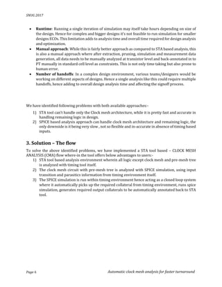
-simulator_type <simulation tool>
-work_dir <simulation directory path>
-preserve <all|fail|none>
#OUTPUT SNIPPET
#Setup mapping of transistor models to gate level models
sim_setup_library
-lib <path to gate level library>
-sub_circuit <Dir path that contains cell sub-circuit file>
-header <path to header files which includes simulation
settings such as model file, corner instantiation and
simulation options>
-file_name_pattern <pattern for input files>
#OUTPUT SNIPPET
#Specify setup option to enable SPICE simulation
sim_setup_spice_deck –enable_clock_mesh
#Test your setup: To validate your SPICE setup is correct, run following commands:-
sim_validate_setup
-from A -to Y
-lib_cell [get_lib_cells $lib_name/<CELL_NAME>]
-capacitance <cap_value> -transition_time <transition_time>

12. SNUG 2017
Page 12 Automatic clock mesh analysis for faster turnaround
Figure 9 Clock mesh model generation flow chart
c) Running CMA flow
#Run spice simulation using sim_analyze_clock_network
#The sim_analyze_clock_network command will extract the clock network from the
specific clock root till the clock pin where clock mesh load cell terminate. It will invoke
the simulator specific by sim_setup_simulator. It creates a spice deck, links to the
simulation environment, runs the simulation and back annotates results on to design in
STA environment.
sim_analyze_clock_network
-from <clock tree root node>
-output <clock_mesh_model.tcl >
#To use or re-use the generated clock mesh model tcl file for design where clock network
is untouched, user can simply run following commands to load it:

13. SNUG 2017
Page 13 Automatic clock mesh analysis for faster turnaround
source clock_mesh_model.tcl
update_timing
4. Results
In this section we are going to describe few metrics to explain objective benefit of CMA based flow as
compared to earlier approach.
Simulation accuracy
To use the flow as signoff tool we need to ensure simulation accuracy matches that of earlier
approach, hence to ensure the generated model is of same or better quality as compared to earlier
approach. In our earlier approach we have used an internal simulator for external simulator while
considering ball park range of input transition and output load as it was not feasible to get right
values at the design stage when circuit team usually optimize the clock mesh.
Hence we are going to describe how CMA flow based simulation numbers fares as compared to
internal simulator. For this we simulated same CMA flow generated spice testbench and netlist, hence
keeping the simulation setup same and only varying the spice models and simulator.
We are considering two type of measurements as below :-
a) Cell delay : We measure cell delay across clock mesh for both rise and fall transition while
varying the input transition values. This process provides us range of cell delays (rise/fall)
values for each of internal simulator and CMA based simulation. We then tabulate the
percentage difference seen between both simulators and plot them against each varying
input transition values as below.
Figure 10: Percentage cell delay difference between both simulators plotted for each of input rise transitions
-0.5
-0.45
-0.4
-0.35
-0.3
-0.25
-0.2
-0.15
-0.1
-0.05
0
Input
trasition
1.00E-10 2.00E-10 5.00E-10 1.00E-09 2.00E-09 5.00E-09 1.00E-08 2.00E-08
Input transitions vs output rise delay diff
percentage

14. SNUG 2017
Page 14 Automatic clock mesh analysis for faster turnaround
Figure 11: Percentage cell delay difference between both simulators plotted for each of input fall transitions
Max Min
Percentage diff range for cell
delay (rise/fall)
0.18% - 1.365%
Figure 12 Summary of simulation result for cell delay
b) Cell transition : We mesure cell transition values at clock mesh output for both rise and fall
input transition while varying the input transition values. This process provides us a range of
cell output transition (rise/fall) values for each of the internal simulator and CMA based
simulation. We then proceed to tabulate the percentage difference seen between both
simulators and plot them against each varying input transition values as below.
-1.6
-1.4
-1.2
-1
-0.8
-0.6
-0.4
-0.2
0
0.2
Input
transition
1.00E-10 2.00E-10 5.00E-10 1.00E-09 2.00E-09 5.00E-09 1.00E-08 2.00E-08
Input transition vs output delay fall diff
percentage

15. SNUG 2017
Page 15 Automatic clock mesh analysis for faster turnaround
Figure 13: Percentage difference in output transition between both simulators plotted for each of input rise transitions
Figure 14: Percentage difference in output transition between both simulators plotted for each of input fall transitions
Max Min
Percentage diff range for cell
transition (rise/fall)
0.355% - 0.885%
Figure 14 Summary of simulation result for cell transition
-0.6
-0.5
-0.4
-0.3
-0.2
-0.1
0
0.1
0.2
0.3
0.4
tran_in_rise 6.00E-11 1.20E-10 3.00E-10 6.00E-10 1.20E-09 3.00E-09 6.00E-09 1.20E-08
input_tran_vs_output_tran_rise
-1
-0.9
-0.8
-0.7
-0.6
-0.5
-0.4
-0.3
-0.2
-0.1
0
tran_in_fall 6.00E-11 1.20E-10 3.00E-10 6.00E-10 1.20E-09 3.00E-09 6.00E-09 1.20E-08
input_tran_vs_output_tran_fall

16. SNUG 2017
Page 16 Automatic clock mesh analysis for faster turnaround
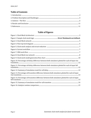
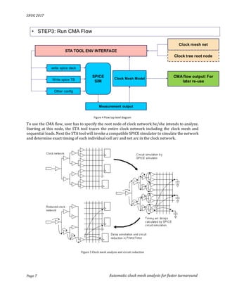
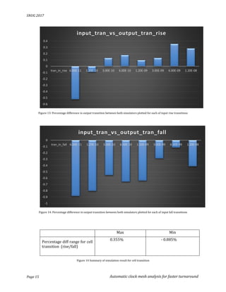
With above data we can conclude between earlier and current approach simulation accuracy for
both cell delay and cell transition is varying by a maximum of 1.365% , which is an acceptable
variation considering this also accounts for differences in spice models and simulators itself.
Analysis runtime
Between earlier and current approach for the testcase, we see a significant improvement in runtime
as below.
Previous approach of CM
analysis
CMA flow based approach
Total analysis time 1 Week 1 hour
Figure 15 : Analysis runtime comparison
5. Conclusions
The implemented flow offers following advantages:-
a) Scalabile yet accurate: The CMA flow is an independent and closed loop flow, hence even
for smallest ECOs there’s no dependency on other teams for collaterals and multiple handoffs.
This methodology can be extended to any number of modes/corners. Though the flow has
some level of limited accuracy , it has been found to be of good enough quality as required for
signoff.
b) Faster turn-around: As compared to existing approach which may take almost a week to
generate the required data to be back-annotated to STA environment, the CMA flow can do it
in few hours, enabling faster design convergence.
CMA Accuracy tradeoff:-
As described earlier, the native STA tool favors clock mesh optimization to reduce clock drivers, this
is to ensure the flow offer faster execution with nominal accuracy loss. This allows more iterations of
ECOs to back annotation within STA tool environment itself. In our analysis we have found the
accuracy level
Hence with above listed advantages of scalability, flexibility and faster turn-around time we were
able to achieve faster and quality design convergence while reducing the resource requirement for
the same task. Moreover the nominal accuracy levels were found to be good enough quality as
required for signoff.
6. References
[1] H. Chen, C. Yeh,G. Wilke, sliding window scheme for accurate clock mesh analysis, ACM library
[2] Pinaki Chakarbarti, Vikram Bhatt, Dwight Hill, Aiqun Cao, Clock mesh framework, ISQED 2012
[3] Malik Devulpalli, Yuichi Kawahara, Clock mesh Variation robustness : Benefit and analysis, Design and
reuse, https://www.design-reuse.com/articles/21019/clock-mesh-benefits-analysis.html
[4] Solvent article: Improved SPICE Correlation Flow.