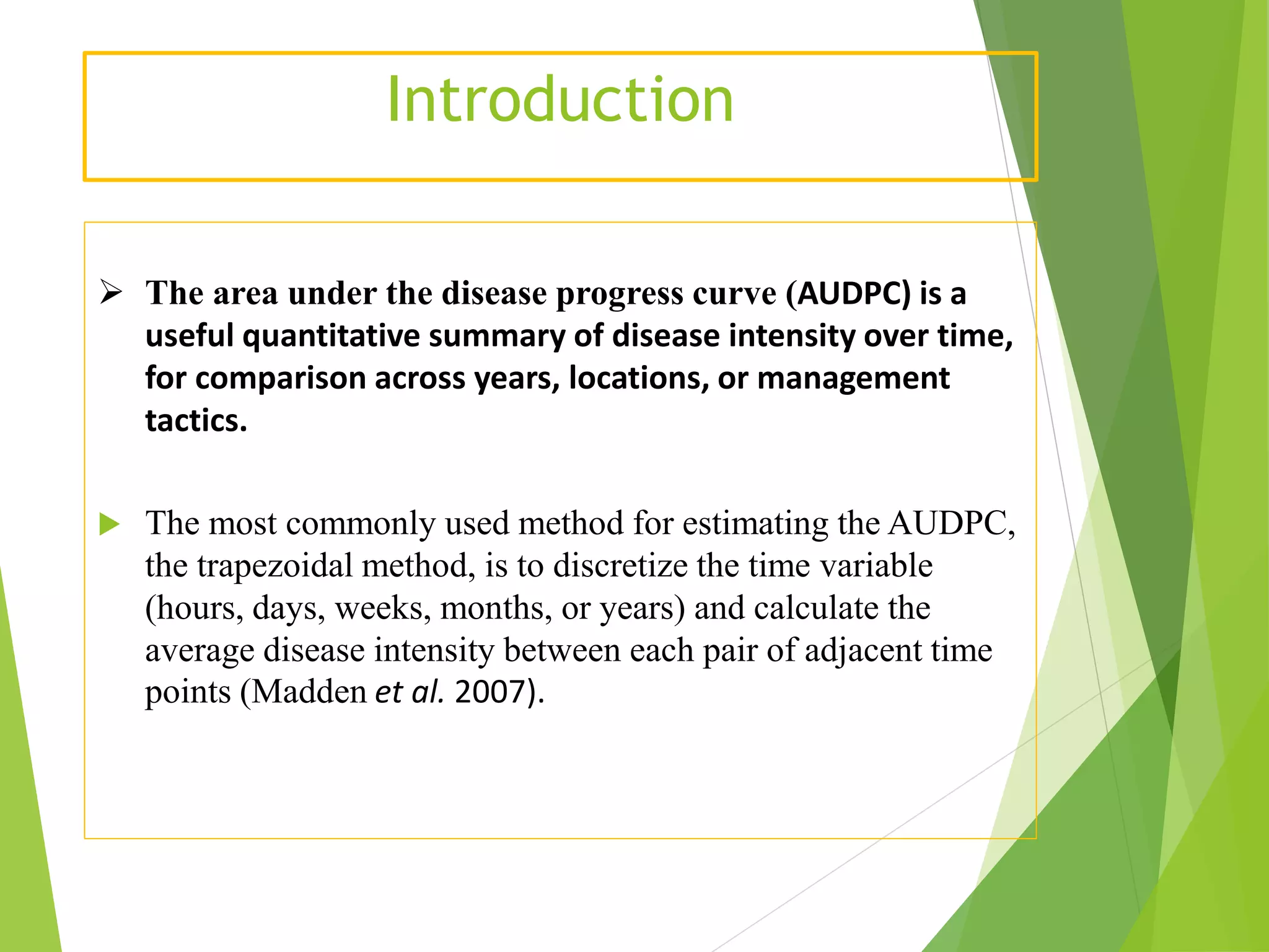
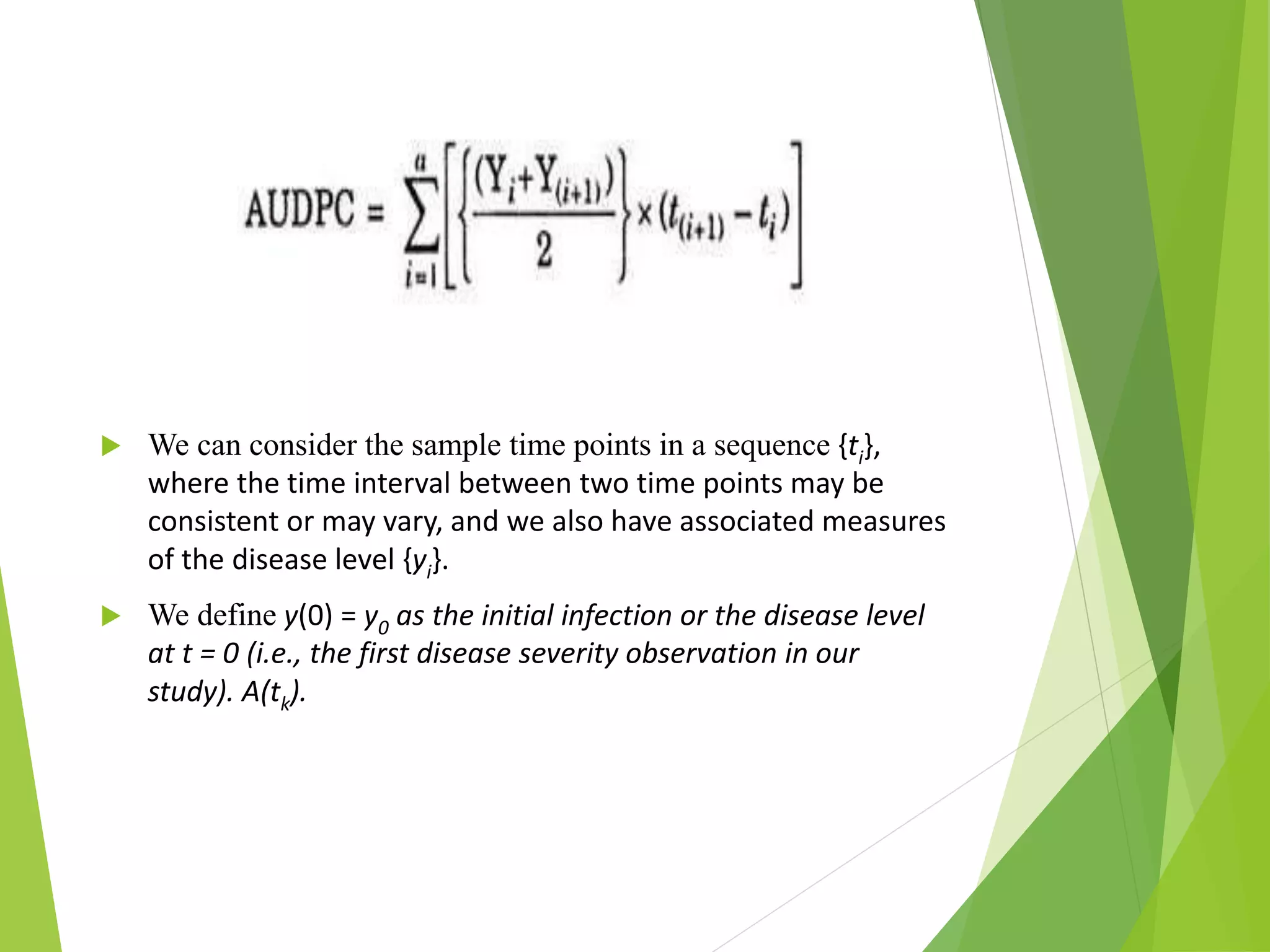
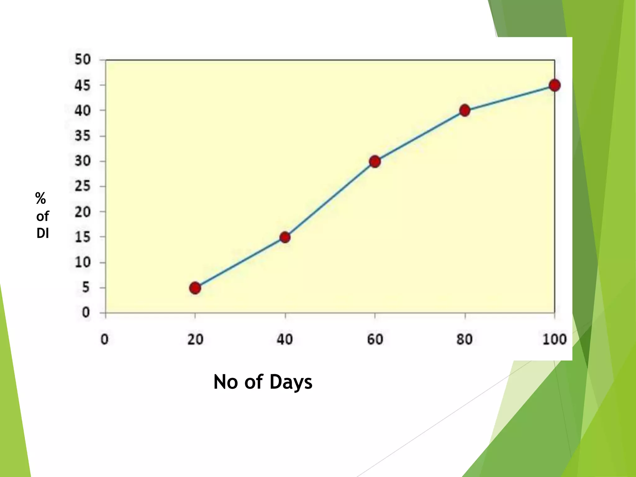
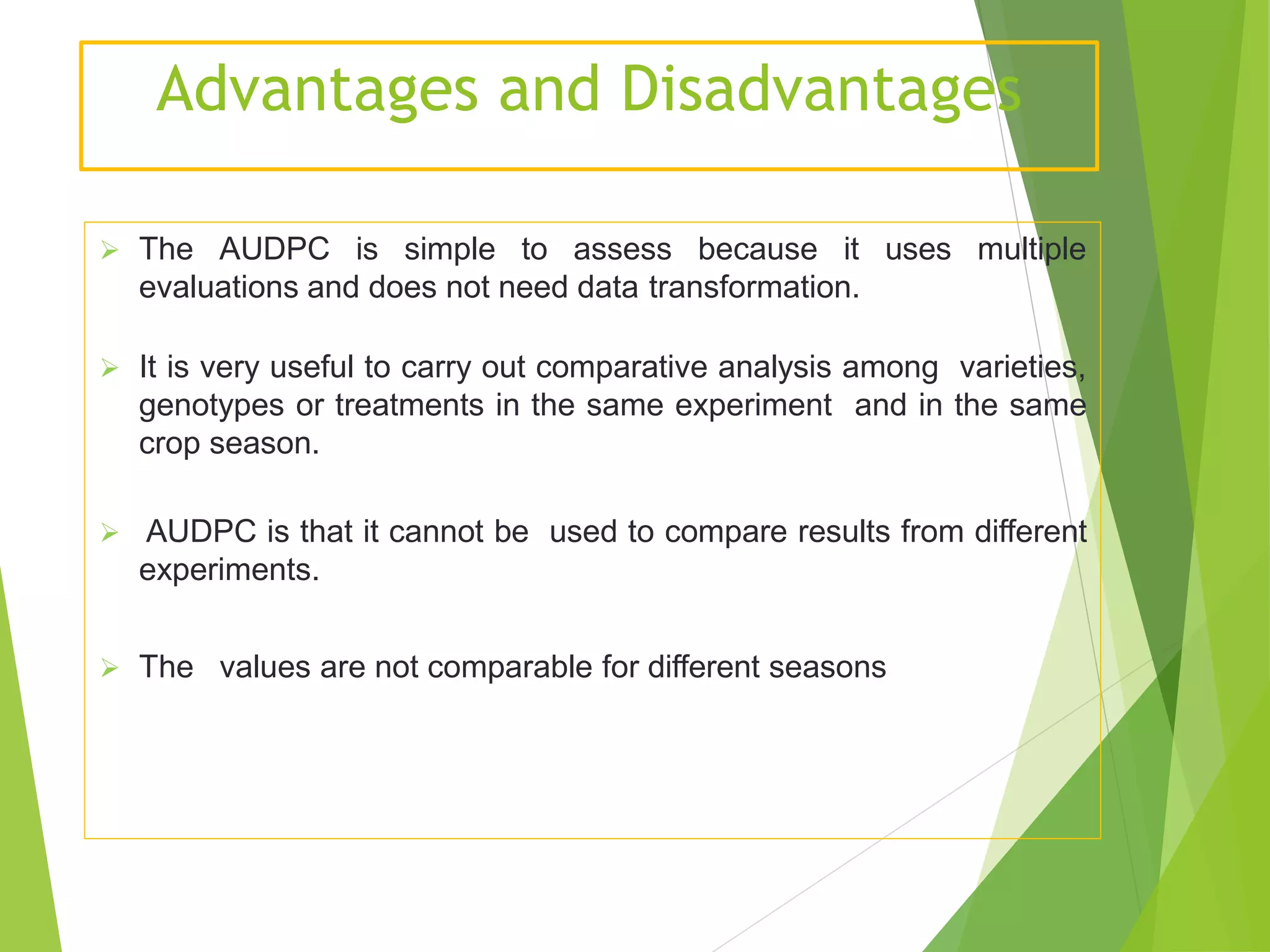
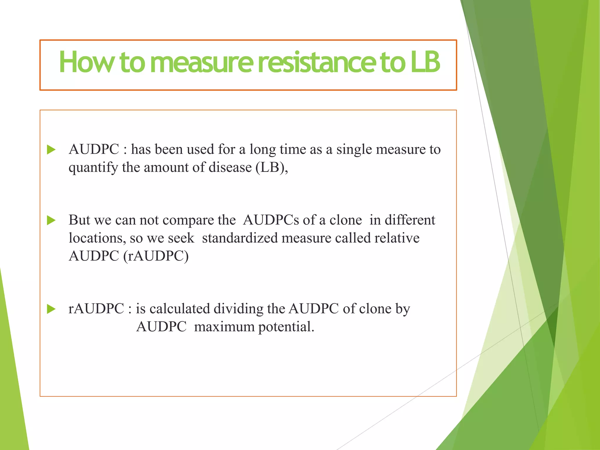
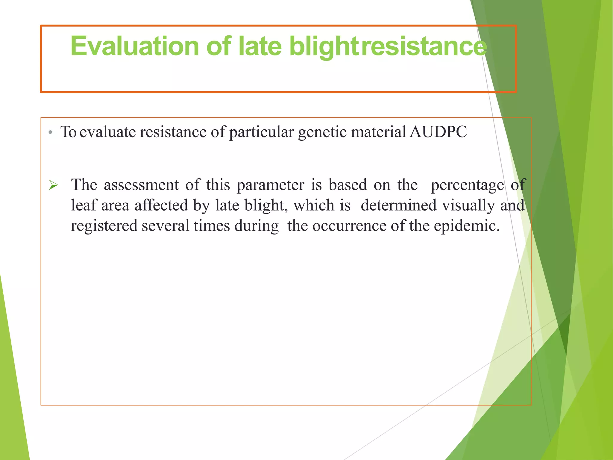
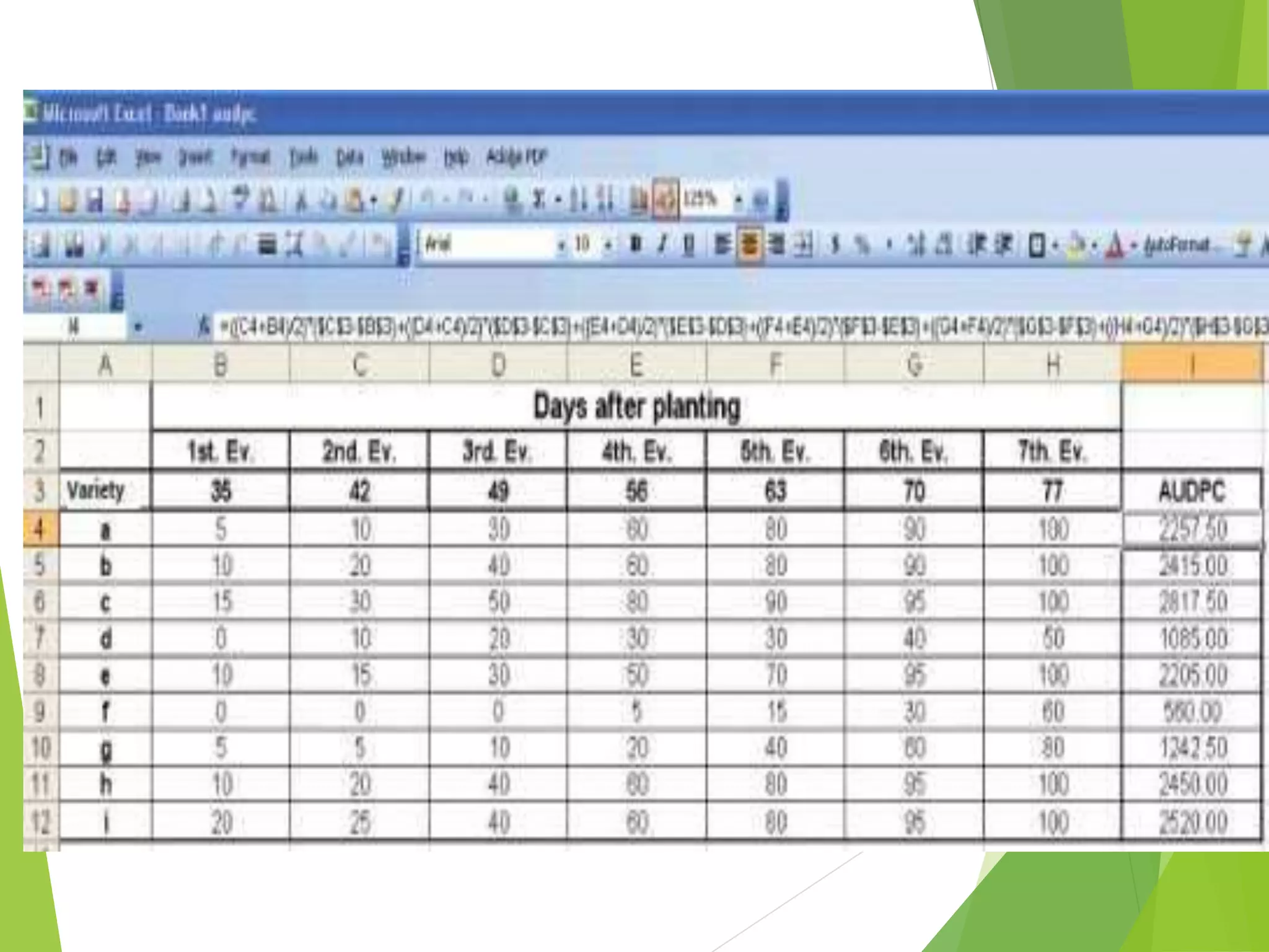
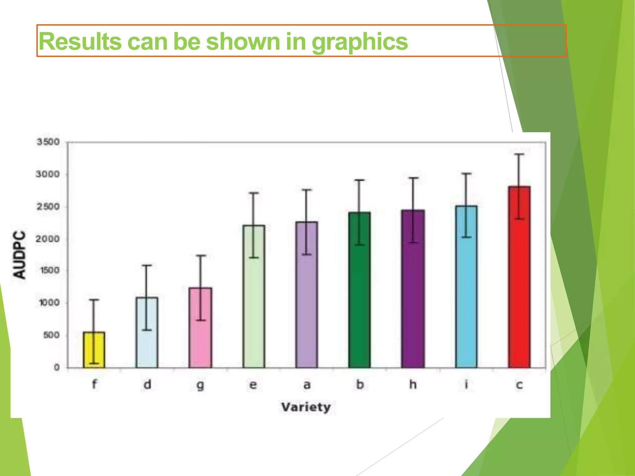
WELCOME
Contents:
 Introduction
 Why we use ?
 How to calculate AUDPC ?
 Advantages of AUDPC
 rAUDPC
 Conclusion
 References
How plant pathogens affect their hosts ?
Effects on host
physiology
Effects on host
development
Effects on yield
quantity
Effects on yield
quality
Time
Diseaseintensity
Time
Yield
Loss
prediction
•For making decision that need of
disease management (cost/effective
calculations).
•For identifying the time when the
control is needed and assisting to
develop effective management
procedures.
•To know the level of resistance of
cultivar against disease
Why we need to evaluate diseases or
assess yield loss?
Methodsforevaluatingdisease
 Horsfall-Barrant Scale: a numeric value are
assigned to the plant according to the percentage
of leaf area infected by the disease.
 Direct Estimation: Estimate percentage of
disease severitydirectly.
Evaluationofdiseasesorquantification
 It is one of the most important tasks
and usually more difficult to perform.
 A adequate evaluation method should give
exact, accurate and reproducibleresults
 Bulky and Laborious to maintain the
data.
Area under disease progress
curve (AUDPC)
Introduction
 The area under the disease progress curve (AUDPC) is a
useful quantitative summary of disease intensity over time,
for comparison across years, locations, or management
tactics.
 The most commonly used method for estimating the AUDPC,
the trapezoidal method, is to discretize the time variable
(hours, days, weeks, months, or years) and calculate the
average disease intensity between each pair of adjacent time
points (Madden et al. 2007).
 We can consider the sample time points in a sequence {ti},
where the time interval between two time points may be
consistent or may vary, and we also have associated measures
of the disease level {yi}.
 We define y(0) = y0 as the initial infection or the disease level
at t = 0 (i.e., the first disease severity observation in our
study). A(tk).
Procedure for Computing the AUDPC
SL
NO
NO OF DAYS PERCENTAGE OF
DISEASE INCIDENCE
1 20 5
2 40 15
3 60 30
4 80 40
5 100 45
%
of
DI
No of Days
%
of
DI
No of Days
No of Days
%
of
DI
AUDPC is estimated by:
 Where,
 n = total number of observations,
 yi = injury intensity (usually incidence in crop health
data) at the i th observation,
 t = time at the i th observation.
Result and Interpretation
Audpc= (0+5/2)*(20-0)+(5+15/2)*(40-
20)+(15+30/2)(60-40)+(30+40/2)*(80-
60)+(40+45/2)*(100-80)
AUDPC=2250%
 AUDPC estimates the area under the disease
progress curve. This value is expressed as %
 Highest values will correspond to more susceptible
varieties and lowest values will correspond to
more resistant varieties.
Advantages and Disadvantages
 The AUDPC is simple to assess because it uses multiple
evaluations and does not need data transformation.
 It is very useful to carry out comparative analysis among varieties,
genotypes or treatments in the same experiment and in the same
crop season.
 AUDPC is that it cannot be used to compare results from different
experiments.
 The values are not comparable for different seasons
HowtomeasureresistancetoLB
 AUDPC : has been used for a long time as a single measure to
quantify the amount of disease (LB),
 But we can not compare the AUDPCs of a clone in different
locations, so we seek standardized measure called relative
AUDPC (rAUDPC)
 rAUDPC : is calculated dividing the AUDPC of clone by
AUDPC maximum potential.
Thescaleofsusceptibility:
 Late blight is a polycyclic disease because the causal agent is
able to reproduce and re-infect other plants in the same crop
season.
 In 2009 Dr. Forbes et al., established a scale of
susceptibility to LB using the numbers 1 to 9.
 This scale allows us to compare resistance of a clones in
different years and locations.
 This scale from 1 to 9 (resistant to susceptible) , gives
numbers that are easier to remember and interpreted
Evaluation of late blightresistance
• Toevaluate resistance of particular genetic material AUDPC
 The assessment of this parameter is based on the percentage of
leaf area affected by late blight, which is determined visually and
registered several times during the occurrence of the epidemic.
Assessment ofAUDPC, a MicrosoftExcel
example
 Evaluations of the percentage of diseased foliar area corresponding to
each genotype according to the date of evaluation should be recorded.
Number of days after planting in which evaluation was per formed must
also be recorded. In the example, nine varieties (a, b, c, d, e, f, g, h, and i)
were evaluated at 7, 14, 21, 28, 35, 42 and 49 days after planting.
1. Place the cursor over cell I4, which corresponds to clone “a” area, and
calculate the AUDPC by using the
 following formula: = ((C4+B4)/2)*($C$3-$B$3)+((D4+C4)/2)*($D$3-
$C$3)+((E4+D4)/2)*($E$3-$D$3)+((F4+E4)/2)*($F$3
$E$3)+((G4+F4)/2)*($G$3-
$F$3)+((H4+G4)/2)*($H$3-$G$3)
3. Press ENTER, and the AUDPC value “2765.00” will be displayed in cell 14
4. Copy cell I4 to the other cells (I5 to I12) and press Edit. Select PASTE
SPECIAL, select FORMULAS and click OK. Values of AUDPC will be
displayed in every copied cell
Results can be shown in graphics
 The relative AUDPC (rAUDPC) should be used to
compare data from different experiments. This value is
better than AUDPC
 it may introduce SOME BAIS as when comparing
experiments.
 To calculate the rAUDPC divide the AUDPC by N,
 where N=(The total number of days between the first and
last evaluation) multiply by100.
Considerations in evaluating
resistance
 Evaluations of the percent of leaf area blighted must be initiated
at the beginning of the epidemic.
 Time intervals for registering should not be long;(1 week) if
climate conditions are favourable to disease development.
 Evaluations should stop when susceptible genotypes are near total
destruction.
 Since susceptible materials cannot get more infected, the more
resistant ones will tend to catch up.
 The date of each evaluation must be recorded .
Uses of the AUDPC models
 The AUDPC models are used in both broad-leaf and cereal
crops.
 In most cases, a very good relationship exist betweenAUDPC
values and yield.
 The AUDPC models are used mainly for “after-season” loss
assessment.
Conclusion
 Statistical models have been used extensively for summarizing and
comparing plant disease epidemics.
 AUDPC was used to illustrate models and to summarize disease
progress over time, in terms of population growth models and
disease progress in a locations.
 AUDPC will help for developing methods to manage plant disease,
such as developing forecasting models to ..
• Selecting an optimal planting date to reduce disease impacts
• To select the planting material.
• Determining the optimal time to apply a fungicide spray.
OR To control disease in upcoming days.
References
 ARPN Journal of Agricultural and Biological Science
 DISEASE PROGRESS CURVES IN THE RICE BLAST
PATHOSYSTEM COMPARED WITH THE LOGISTIC AND
GOMPERTZ MODELS -N. K. Mohapatra
 Google.com
Audpc

Audpc

  • 1.
  • 2.
    Contents:  Introduction  Whywe use ?  How to calculate AUDPC ?  Advantages of AUDPC  rAUDPC  Conclusion  References
  • 4.
    How plant pathogensaffect their hosts ? Effects on host physiology Effects on host development Effects on yield quantity Effects on yield quality
  • 5.
    Time Diseaseintensity Time Yield Loss prediction •For making decisionthat need of disease management (cost/effective calculations). •For identifying the time when the control is needed and assisting to develop effective management procedures. •To know the level of resistance of cultivar against disease Why we need to evaluate diseases or assess yield loss?
  • 6.
    Methodsforevaluatingdisease  Horsfall-Barrant Scale:a numeric value are assigned to the plant according to the percentage of leaf area infected by the disease.  Direct Estimation: Estimate percentage of disease severitydirectly.
  • 7.
    Evaluationofdiseasesorquantification  It isone of the most important tasks and usually more difficult to perform.  A adequate evaluation method should give exact, accurate and reproducibleresults  Bulky and Laborious to maintain the data.
  • 8.
    Area under diseaseprogress curve (AUDPC)
  • 9.
    Introduction  The areaunder the disease progress curve (AUDPC) is a useful quantitative summary of disease intensity over time, for comparison across years, locations, or management tactics.  The most commonly used method for estimating the AUDPC, the trapezoidal method, is to discretize the time variable (hours, days, weeks, months, or years) and calculate the average disease intensity between each pair of adjacent time points (Madden et al. 2007).
  • 10.
     We canconsider the sample time points in a sequence {ti}, where the time interval between two time points may be consistent or may vary, and we also have associated measures of the disease level {yi}.  We define y(0) = y0 as the initial infection or the disease level at t = 0 (i.e., the first disease severity observation in our study). A(tk).
  • 11.
    Procedure for Computingthe AUDPC SL NO NO OF DAYS PERCENTAGE OF DISEASE INCIDENCE 1 20 5 2 40 15 3 60 30 4 80 40 5 100 45
  • 12.
  • 13.
  • 14.
  • 15.
    AUDPC is estimatedby:  Where,  n = total number of observations,  yi = injury intensity (usually incidence in crop health data) at the i th observation,  t = time at the i th observation.
  • 16.
    Result and Interpretation Audpc=(0+5/2)*(20-0)+(5+15/2)*(40- 20)+(15+30/2)(60-40)+(30+40/2)*(80- 60)+(40+45/2)*(100-80) AUDPC=2250%  AUDPC estimates the area under the disease progress curve. This value is expressed as %  Highest values will correspond to more susceptible varieties and lowest values will correspond to more resistant varieties.
  • 17.
    Advantages and Disadvantages The AUDPC is simple to assess because it uses multiple evaluations and does not need data transformation.  It is very useful to carry out comparative analysis among varieties, genotypes or treatments in the same experiment and in the same crop season.  AUDPC is that it cannot be used to compare results from different experiments.  The values are not comparable for different seasons
  • 18.
    HowtomeasureresistancetoLB  AUDPC :has been used for a long time as a single measure to quantify the amount of disease (LB),  But we can not compare the AUDPCs of a clone in different locations, so we seek standardized measure called relative AUDPC (rAUDPC)  rAUDPC : is calculated dividing the AUDPC of clone by AUDPC maximum potential.
  • 19.
    Thescaleofsusceptibility:  Late blightis a polycyclic disease because the causal agent is able to reproduce and re-infect other plants in the same crop season.  In 2009 Dr. Forbes et al., established a scale of susceptibility to LB using the numbers 1 to 9.  This scale allows us to compare resistance of a clones in different years and locations.  This scale from 1 to 9 (resistant to susceptible) , gives numbers that are easier to remember and interpreted
  • 20.
    Evaluation of lateblightresistance • Toevaluate resistance of particular genetic material AUDPC  The assessment of this parameter is based on the percentage of leaf area affected by late blight, which is determined visually and registered several times during the occurrence of the epidemic.
  • 21.
    Assessment ofAUDPC, aMicrosoftExcel example  Evaluations of the percentage of diseased foliar area corresponding to each genotype according to the date of evaluation should be recorded. Number of days after planting in which evaluation was per formed must also be recorded. In the example, nine varieties (a, b, c, d, e, f, g, h, and i) were evaluated at 7, 14, 21, 28, 35, 42 and 49 days after planting. 1. Place the cursor over cell I4, which corresponds to clone “a” area, and calculate the AUDPC by using the  following formula: = ((C4+B4)/2)*($C$3-$B$3)+((D4+C4)/2)*($D$3- $C$3)+((E4+D4)/2)*($E$3-$D$3)+((F4+E4)/2)*($F$3 $E$3)+((G4+F4)/2)*($G$3- $F$3)+((H4+G4)/2)*($H$3-$G$3) 3. Press ENTER, and the AUDPC value “2765.00” will be displayed in cell 14 4. Copy cell I4 to the other cells (I5 to I12) and press Edit. Select PASTE SPECIAL, select FORMULAS and click OK. Values of AUDPC will be displayed in every copied cell
  • 24.
    Results can beshown in graphics
  • 25.
     The relativeAUDPC (rAUDPC) should be used to compare data from different experiments. This value is better than AUDPC  it may introduce SOME BAIS as when comparing experiments.  To calculate the rAUDPC divide the AUDPC by N,  where N=(The total number of days between the first and last evaluation) multiply by100.
  • 26.
    Considerations in evaluating resistance Evaluations of the percent of leaf area blighted must be initiated at the beginning of the epidemic.  Time intervals for registering should not be long;(1 week) if climate conditions are favourable to disease development.  Evaluations should stop when susceptible genotypes are near total destruction.  Since susceptible materials cannot get more infected, the more resistant ones will tend to catch up.  The date of each evaluation must be recorded .
  • 27.
    Uses of theAUDPC models  The AUDPC models are used in both broad-leaf and cereal crops.  In most cases, a very good relationship exist betweenAUDPC values and yield.  The AUDPC models are used mainly for “after-season” loss assessment.
  • 28.
    Conclusion  Statistical modelshave been used extensively for summarizing and comparing plant disease epidemics.  AUDPC was used to illustrate models and to summarize disease progress over time, in terms of population growth models and disease progress in a locations.  AUDPC will help for developing methods to manage plant disease, such as developing forecasting models to .. • Selecting an optimal planting date to reduce disease impacts • To select the planting material. • Determining the optimal time to apply a fungicide spray. OR To control disease in upcoming days.
  • 29.
    References  ARPN Journalof Agricultural and Biological Science  DISEASE PROGRESS CURVES IN THE RICE BLAST PATHOSYSTEM COMPARED WITH THE LOGISTIC AND GOMPERTZ MODELS -N. K. Mohapatra  Google.com