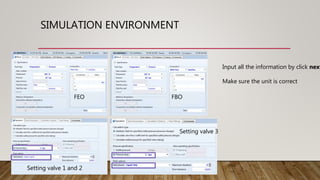
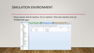
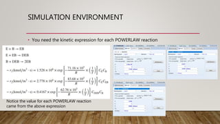
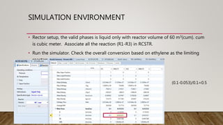
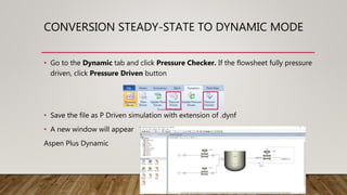
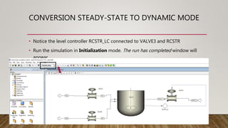
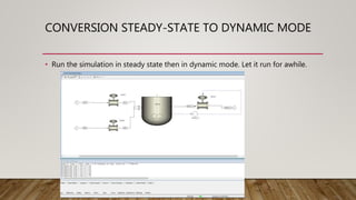
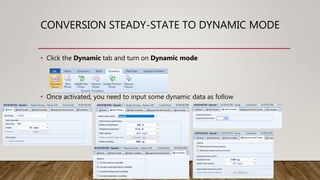
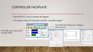
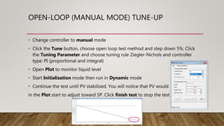
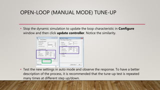
This document describes using ASPEN Plus dynamic simulation software to model and control a continuous stirred tank reactor (CSTR) process. It introduces key dynamic simulation concepts and outlines the steps to: 1) Build a process flowsheet model in steady-state, including reactions, streams and equipment. 2) Convert the model to dynamic mode and input dynamic parameters. 3) Add a level controller to the CSTR and tune it using open-loop testing and the Ziegler-Nichols method. 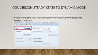4) Simulate the dynamic behavior of the controlled process to evaluate controller performance.

1. ASPEN PLUS
DYNAMIC
KHAIRUL ANWAR MOHAMAD SAID

2. INTRODUCTION
• It is a process control
• ASPEN dynamic simulate a process by running it within a controlled variable
• Basic term:
• Open loop control: controller output has no feedback from the process itself and
manually change by the operator. Controller fixed at a value
• Disturbance: uncontrolled changes which affect the process variable
• Close loop control: controller output has feedback from the process.
• PV: present value, SP: set point, OP: output (controller)

3. DESCRIPTION
• Ethylbenzene (E) react with benzene (B) to produce desired product ethylbenzene
(EB). There is a consecutive reaction that produces the undesirable product
diethylbenzene (DEB). The third reaction combine benzene and diethylbenzene to
form ethylbenzene
1)
2)
3)

4. CONTINUE
• In symbolic notation:
• k is second order reaction constant (m3/kmol.s). Concentration in mol/l or
kmol/m3. Activation energy in kJ/kmol. Temperature in Kelvin.

5. CONTINUE
• Two feed stream enter the reactor with 0.1 kmol/s ethylene and 0.2 kmol/s
benzene. Notice that molar flow rate of benzene is more than its stoichiometric
value to maintain low enthylene concentration which minimized DEB formation.
DEB is undesired product.

6. PROPERTIES ENVIRONMENT
• Template “chemical with metric units” and change unit to SI in global

7. PROPERTIES ENVIRONMENT
• Add m-DEB (m-diethylbenzene) and other chemicals
• PSRK as the property method, click next and run the properties.

8. SIMULATION ENVIRONMENT
• Follow the following process flowsheet

9. SIMULATION ENVIRONMENT
Setting valve 1 and 2
Setting valve 3
FBO
FEO
Input all the information by click next
Make sure the unit is correct

10. • Setup reactor and its reaction. Go to reaction. Click new reaction and use
POWERLAW type.
SIMULATION ENVIRONMENT

11. SIMULATION ENVIRONMENT
• You need the kinetic expression for each POWERLAW reaction
Notice the value for each POWERLAW reaction
came from the above expression

12. SIMULATION ENVIRONMENT
• Rector setup, the valid phases is liquid only with reactor volume of 60 m3(cum). cum
is cubic meter. Associate all the reaction (R1-R3) in RCSTR.
• Run the simulator. Check the overall conversion based on ethylene as the limiting
reactant
(0.1-0.053)/0.1=0.5

13. CONVERSION STEADY-STATE TO DYNAMIC MODE
• Click the Dynamic tab and turn on Dynamic mode
• Once activated, you need to input some dynamic data as follow

14. CONVERSION STEADY-STATE TO DYNAMIC MODE
• Before running the simulation, change convergence solver from Broyden to
Newton. Then run it

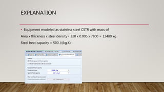
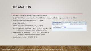
15. EXPLANATION
• Temperature approach is LMTD, logarithmic mean temperature difference.
• LMTD=[(400-298)-(400-343)]/ln(102/57)]=77.33K; heat capacity water 4200J/kg.K
• 400 K refer to reactor temperature which need to maintain. 298 and 343 K refer to
coolant temperature enter and leave the jacket.

16. EXPLANATION
• Equipment modeled as stainless steel CSTR with mass of
Area x thickness x steel density= 320 x 0.005 x 7800 = 12480 kg
Steel heat capacity = 500 J/(kg.K)

17. EXPLANATION
• Q=UA∆T=3.71018x106 W= UA x 77.33 K; UA= 47979 W/K
• U=150 W/m2.K from industrial cooler with cold fluid as water and hot fluid as organic solvent*. So, A= 320 m2
• V= π x (D2/4) x L= 60 = π x (D2/4) x 10; D = 2.764 m
• Area = πDL=86.83 m2
• Lateral area= 320 = π x 0.1016 x Lcoil ; Lcoil = 3150 m
• Lcoil=Nloop x Length single loop = Nloop x π x 0.95 x Dtank ;Nloop=382
• 0.95 for clearance between reactor wall and coil surface
• Vertical space for entire loop = 1.25 x 0.1016 x 382 = 48.51 m.
• 1.25 clearance factor between one loop and another
• Liquid volume fraction= 48.51/10 = 0.485
*https://www.engineersedge.com/thermodynamics/overall_heat_transfer-table.htm

18. CONVERSION STEADY-STATE TO DYNAMIC MODE
• Go to the Dynamic tab and click Pressure Checker. If the flowsheet fully pressure
driven, click Pressure Driven button
• Save the file as P Driven simulation with extension of .dynf
• A new window will appear
Aspen Plus Dynamic

19. CONVERSION STEADY-STATE TO DYNAMIC MODE
• Notice the level controller RCSTR_LC connected to VALVE3 and RCSTR
• Run the simulation in Initialization mode. The run has completed window will
appear.

20. CONVERSION STEADY-STATE TO DYNAMIC MODE
• Run the simulation in steady state then in dynamic mode. Let it run for awhile.

21. CONTROLLER FACEPLATE
• Click RCSTR_LC and a window will appear.
• PV: present value, SP: set point and OP: controller output
From left: auto, manual and
cascade mode
From left: Percentage unit, configure,
plot and tune

22. OPEN-LOOP (MANUAL MODE) TUNE-UP
• Change controller to manual mode
• Click the Tune button, choose open loop test method and step down 5%. Click
the Tuning Parameter and choose tuning rule Ziegler-Nichols and controller
type: PI (proportional and integral)
• Open Plot to monitor liquid level
• Start Initialization mode then run in Dynamic mode
• Continue the test until PV stabilized. You will notice that PV would
in the Plot start to adjust toward SP. Click finish test to stop the test

23. OPEN-LOOP (MANUAL MODE) TUNE-UP
• After the test finish, Tune window will show the estimated control loop
characteristic
• Go to Tuning parameters, click calculate. You will get value for gain and integral
time for PI controller based on Ziegler-Nichols tuning rule

24. OPEN-LOOP (MANUAL MODE) TUNE-UP
• Stop the dynamic simulation to update the loop characteristic in Configure
window and then click update controller. Notice the similarity.
• Test the new settings in auto mode and observe the response. To have a better
description of the process, it is recommended that the tune-up test is repeated
many times at different step up/down.

25. THANK YOU