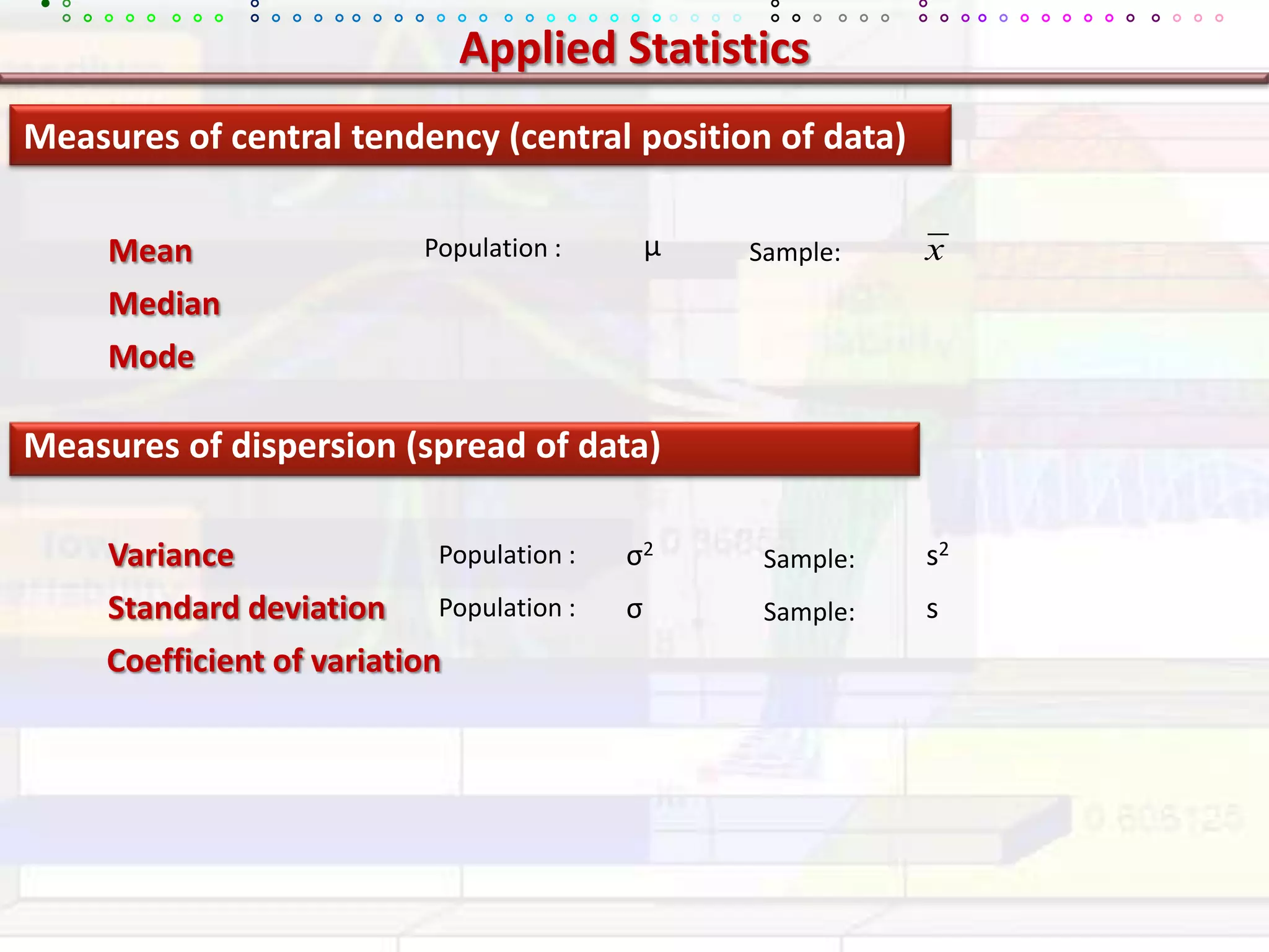
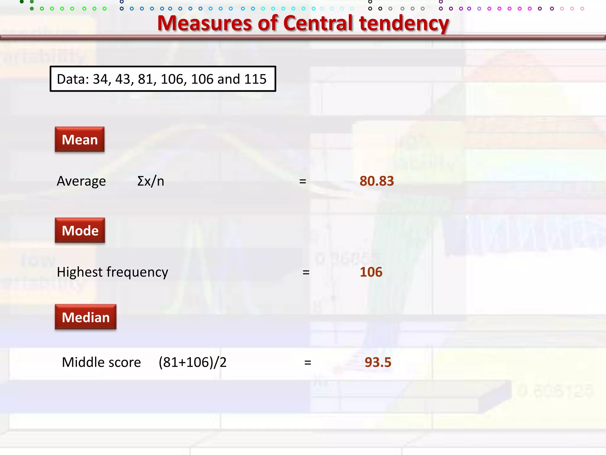
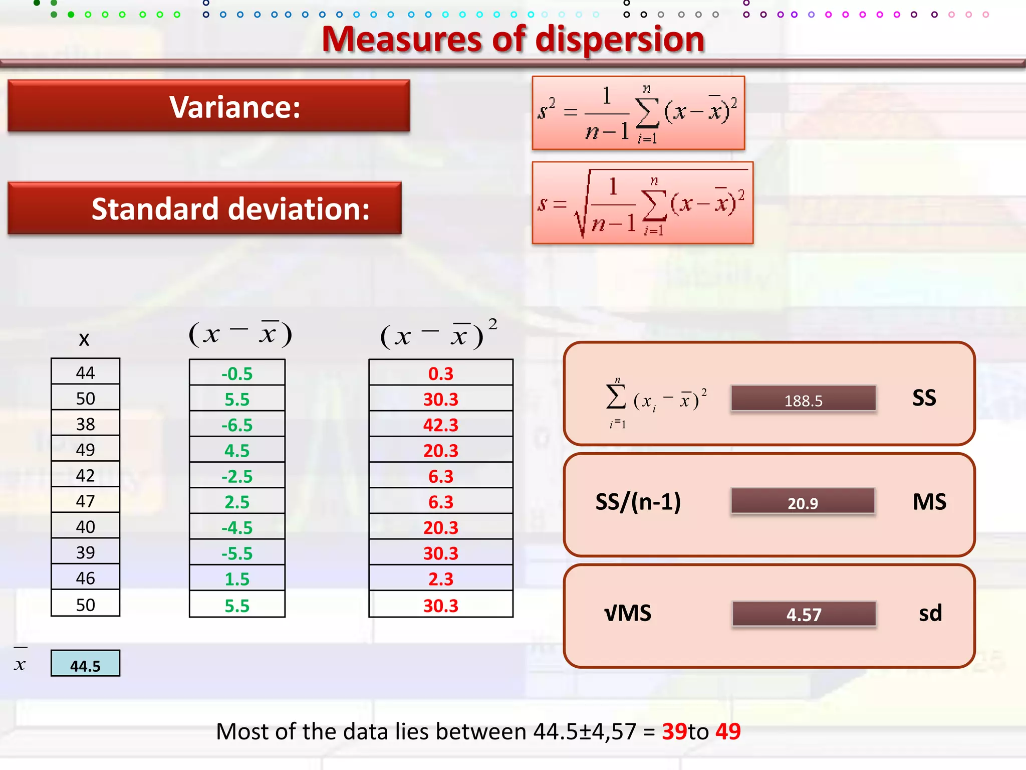
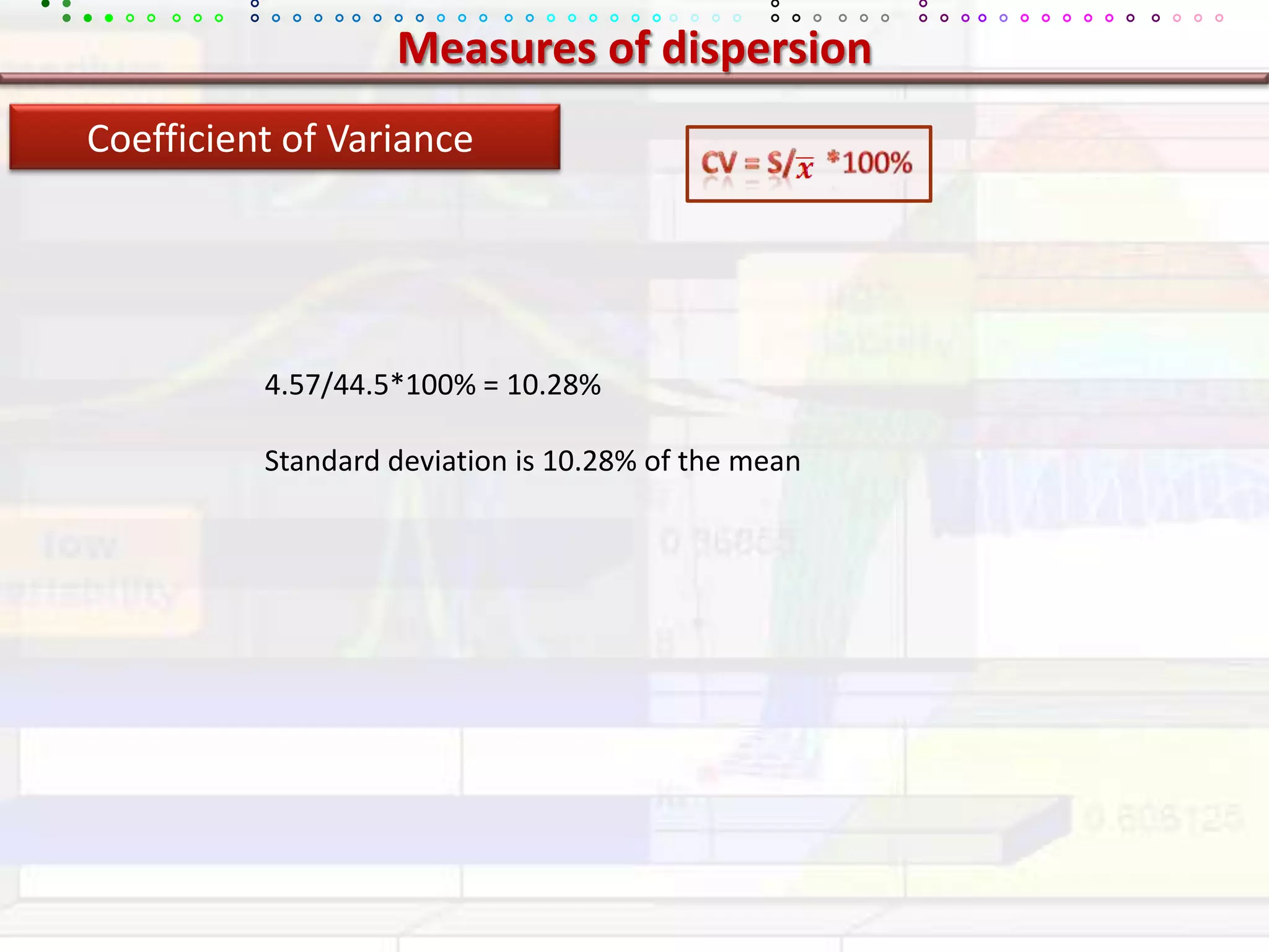
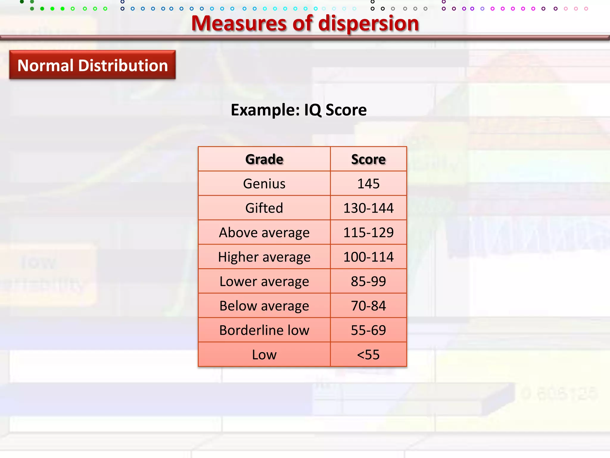
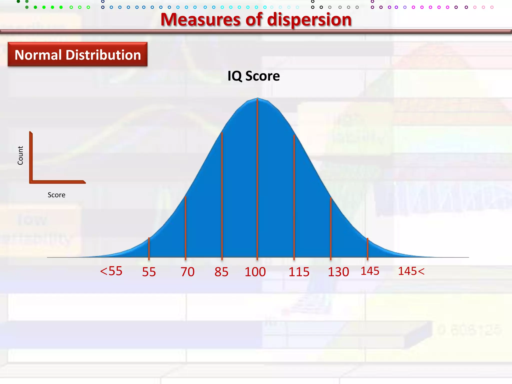
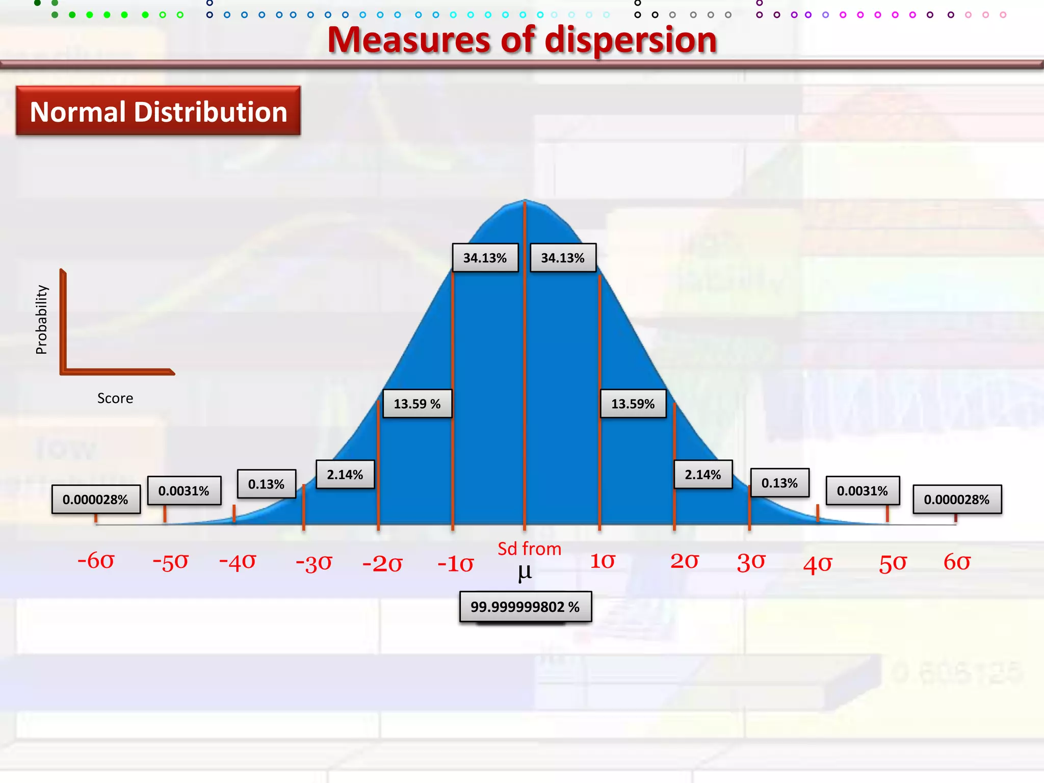
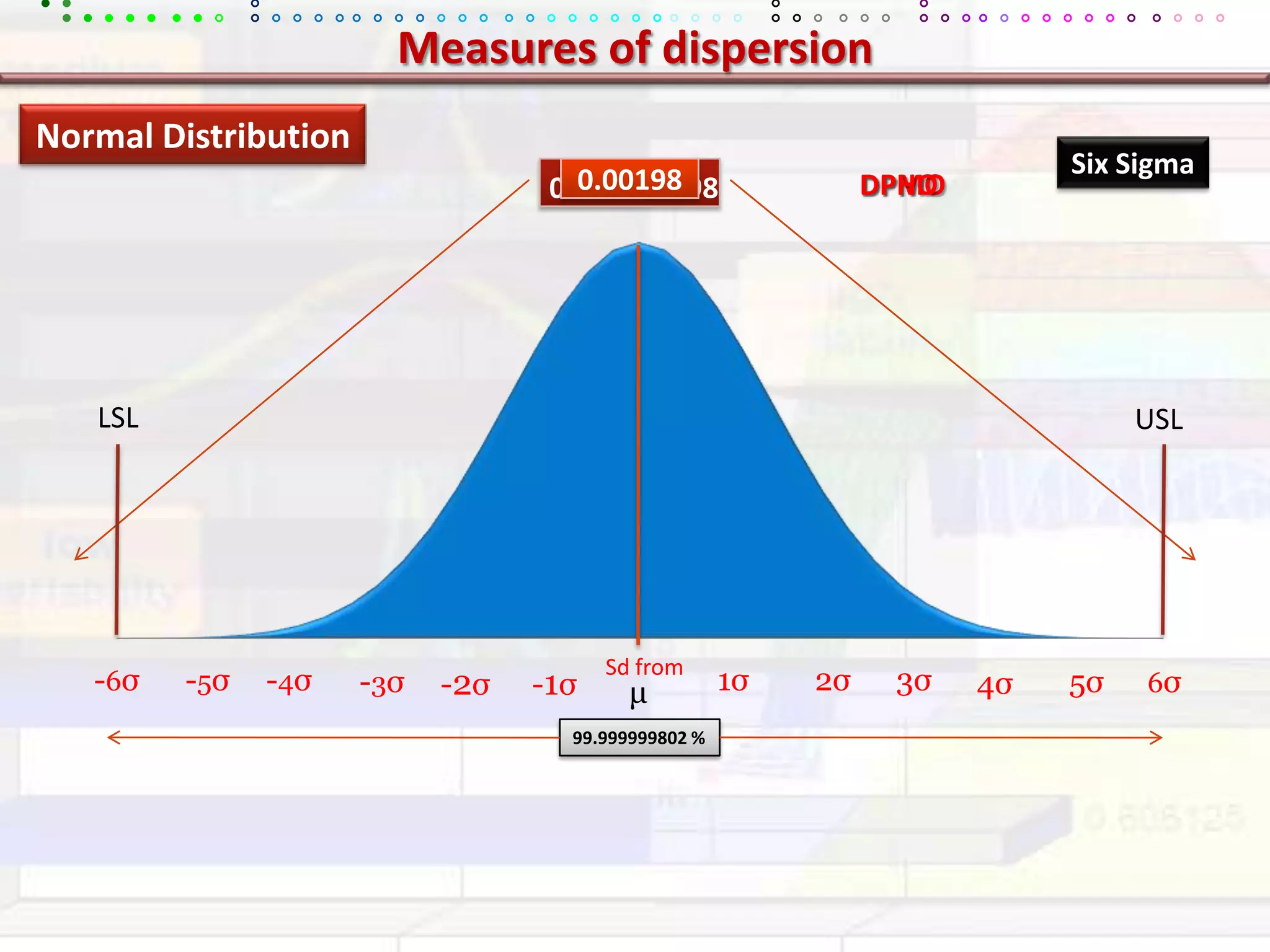
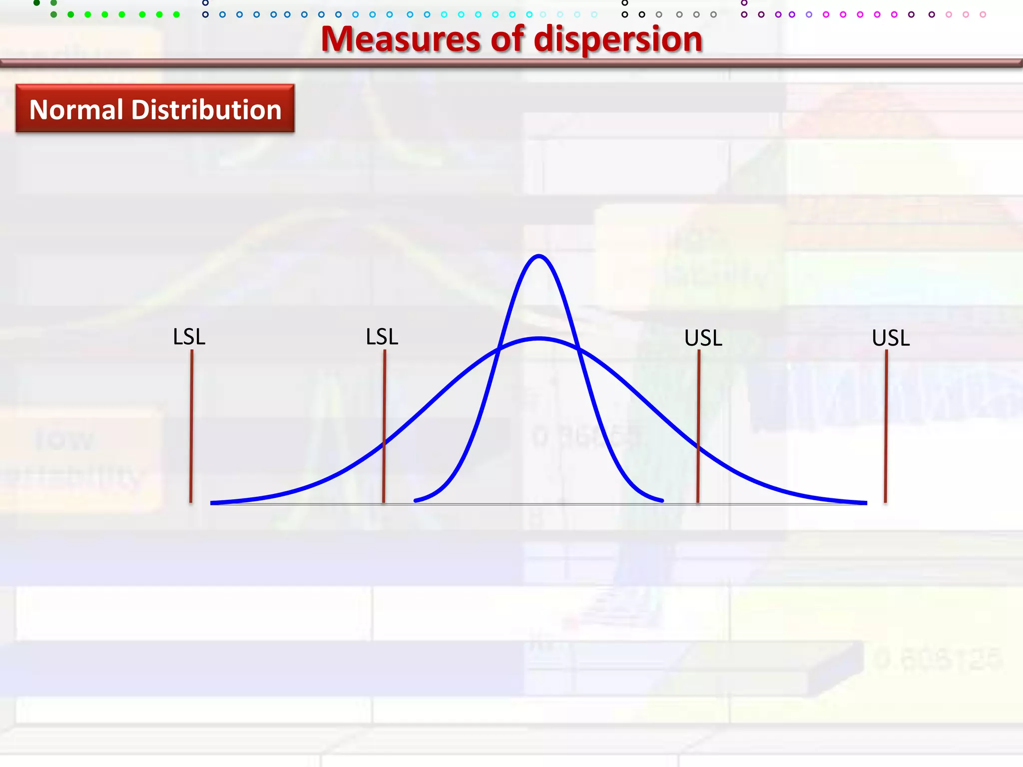
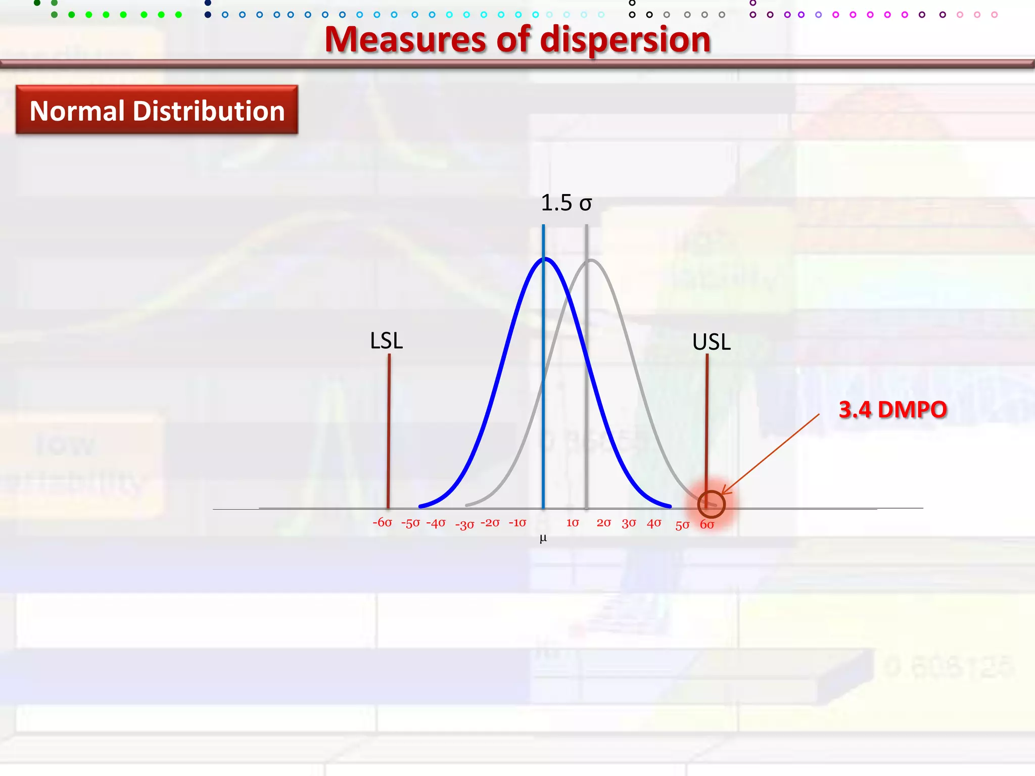
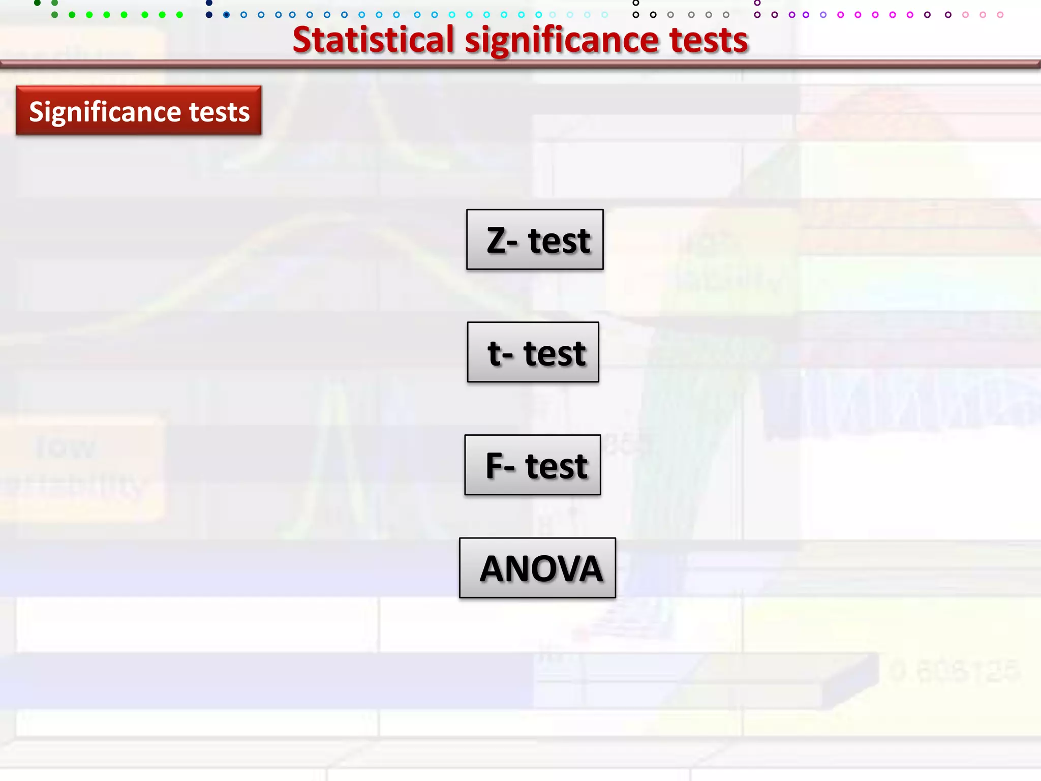
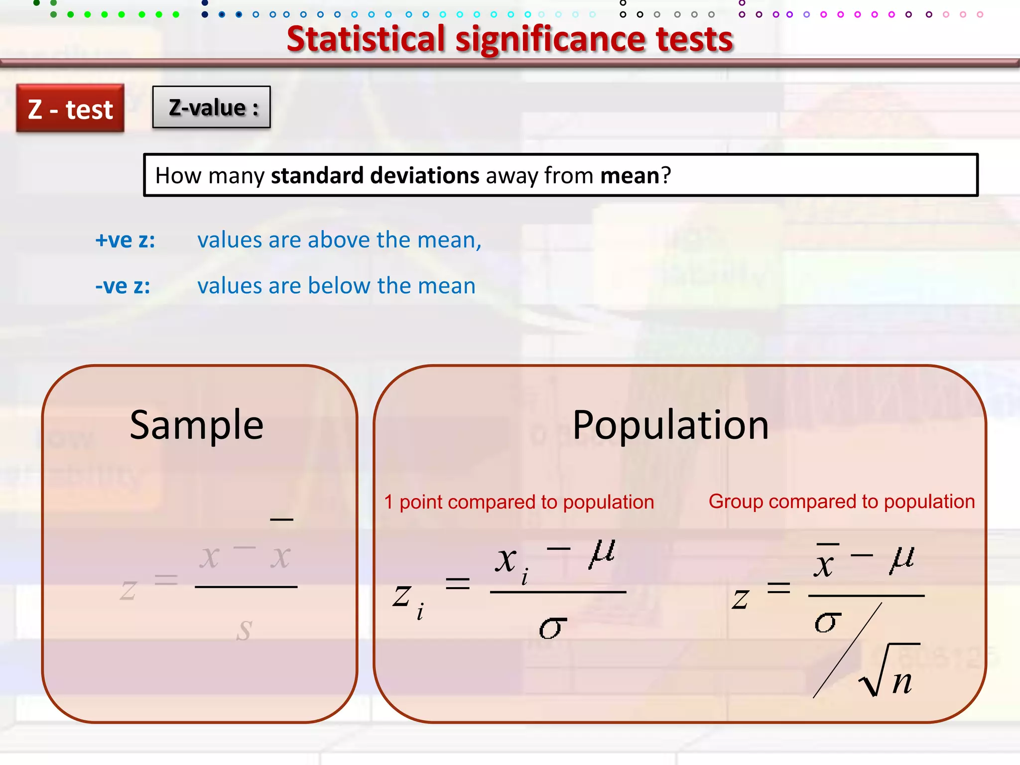
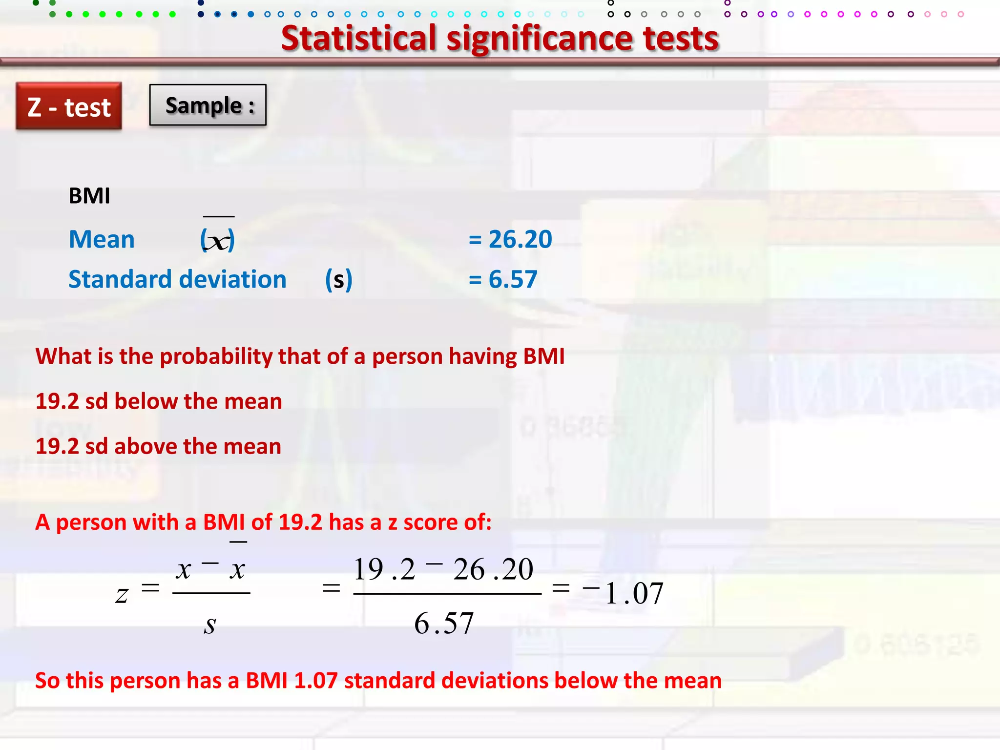
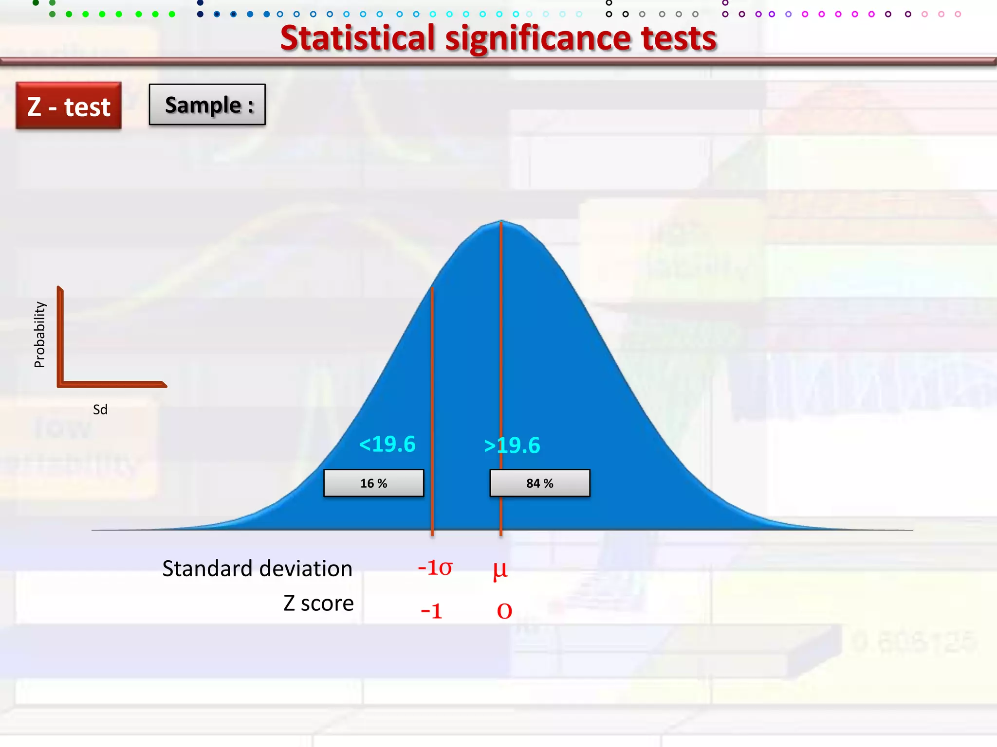
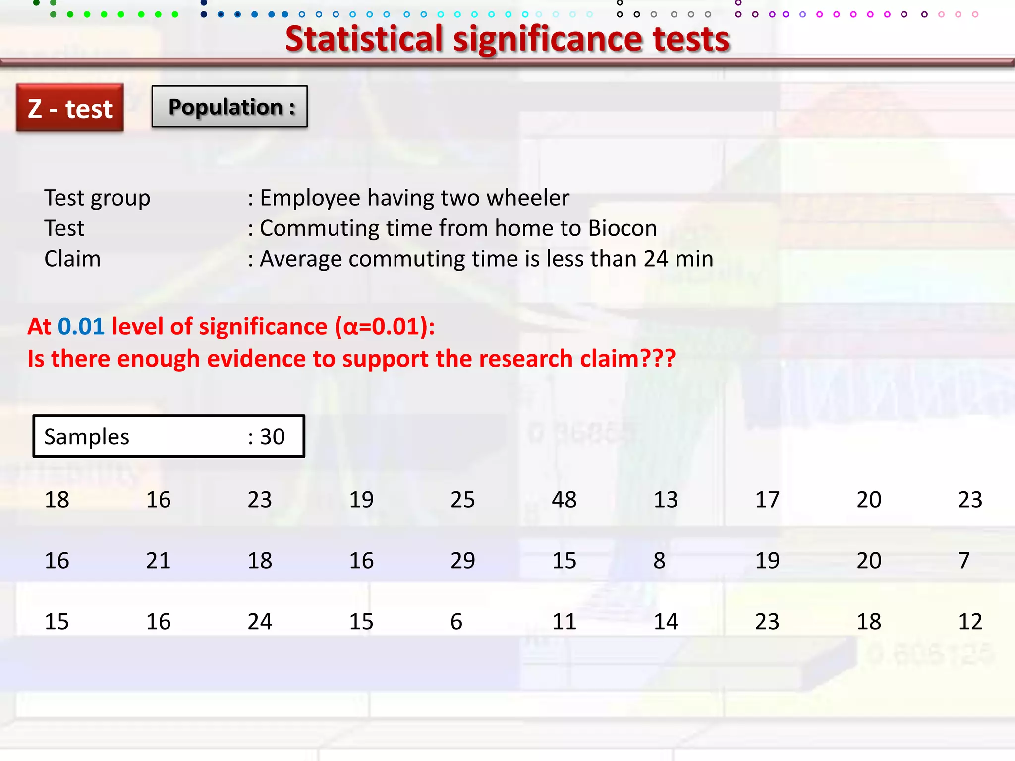
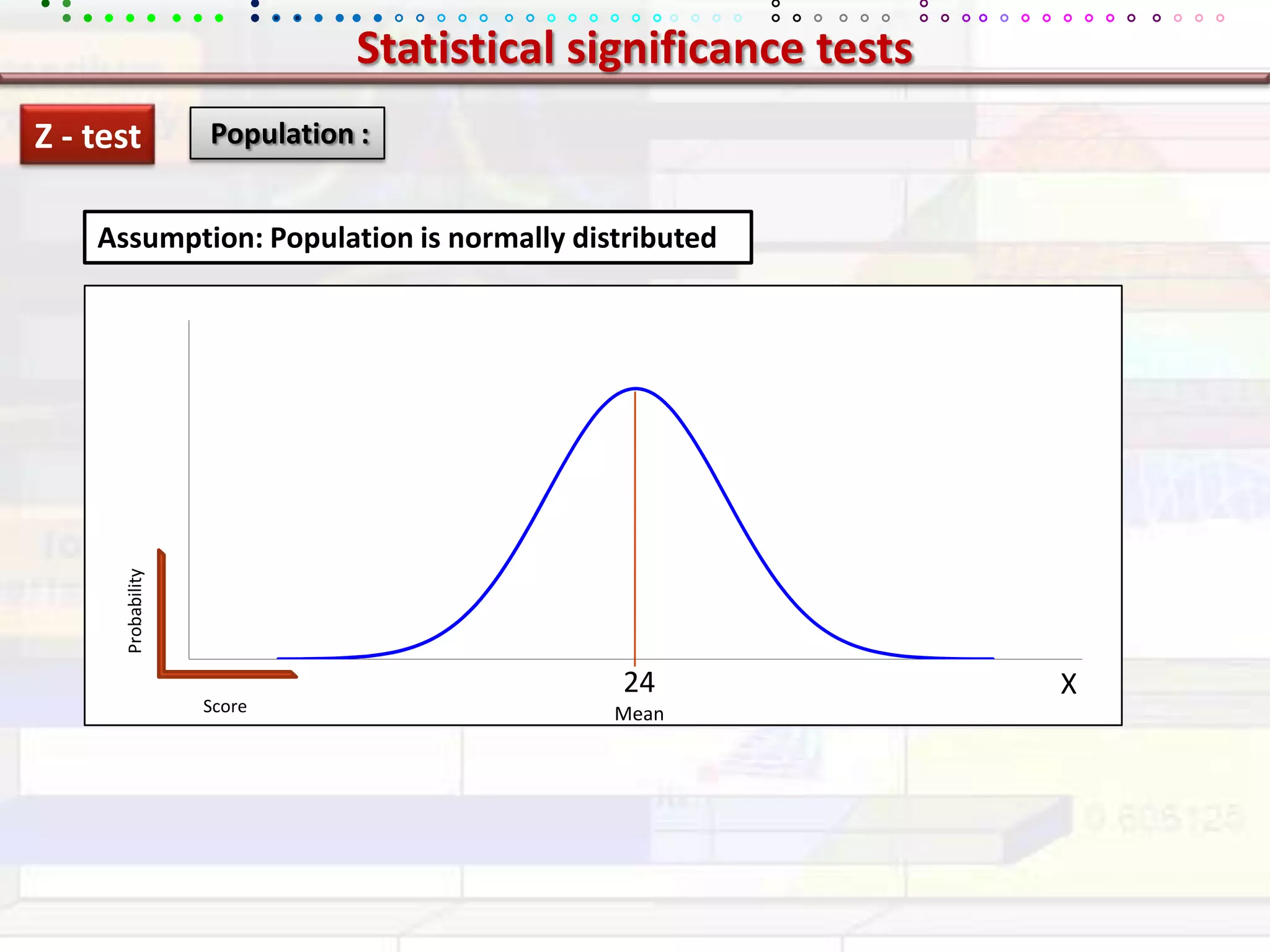
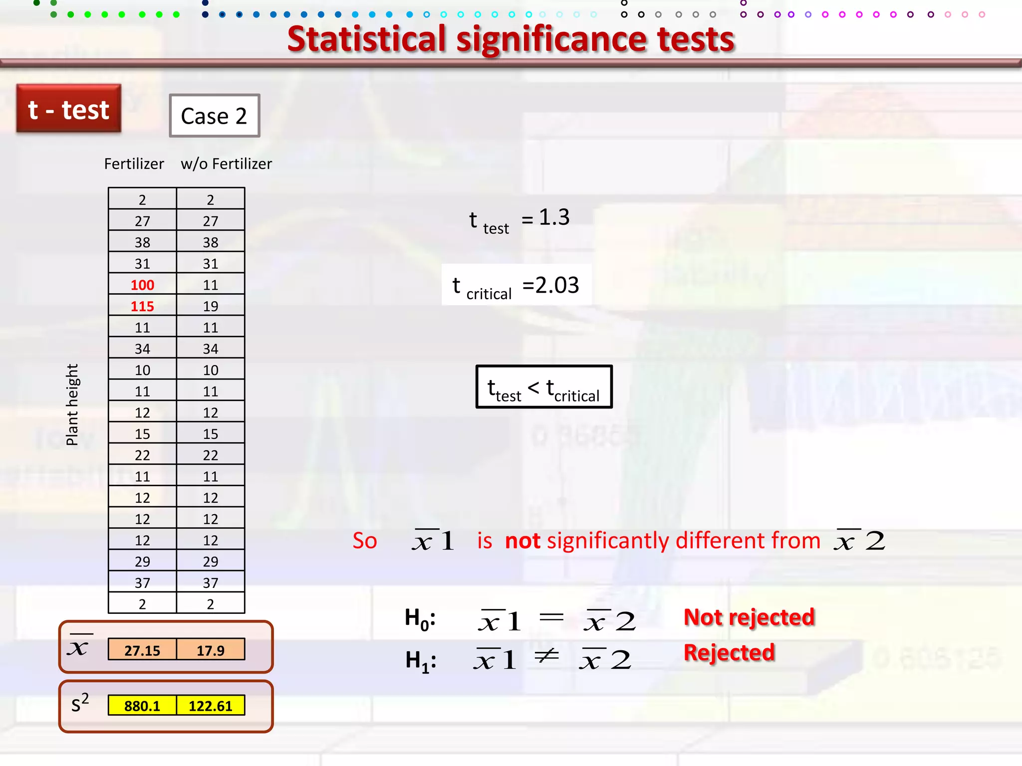
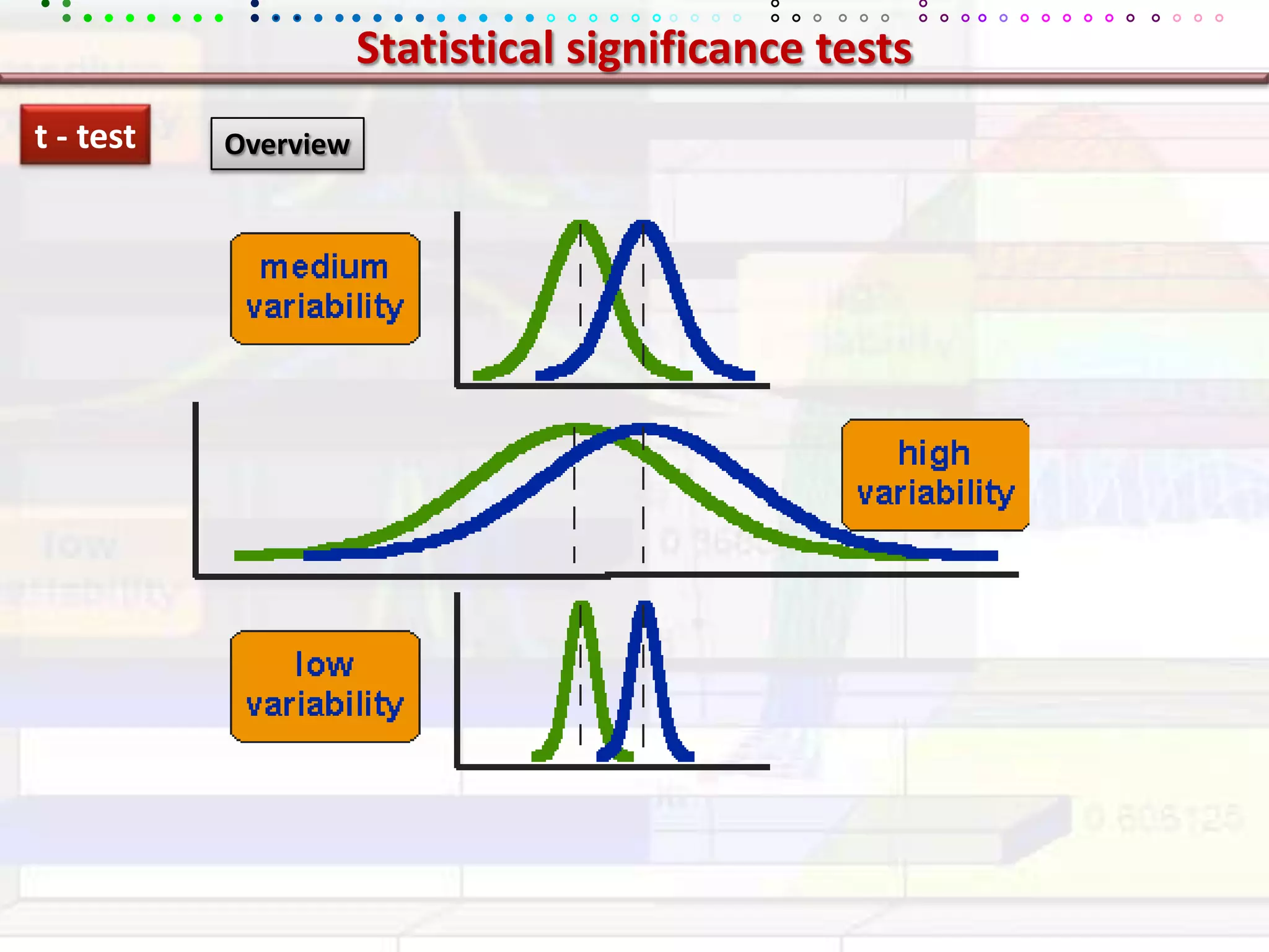
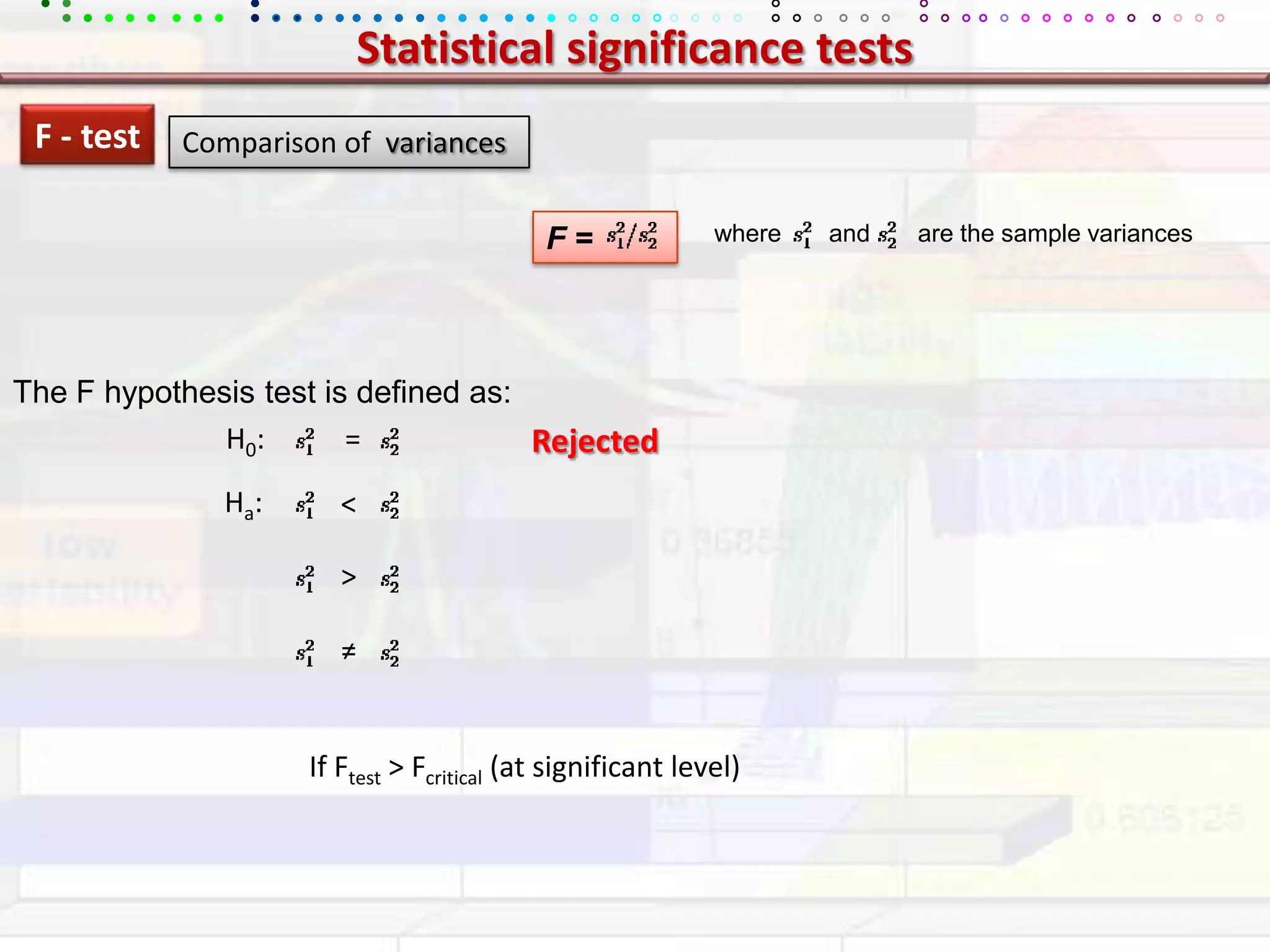
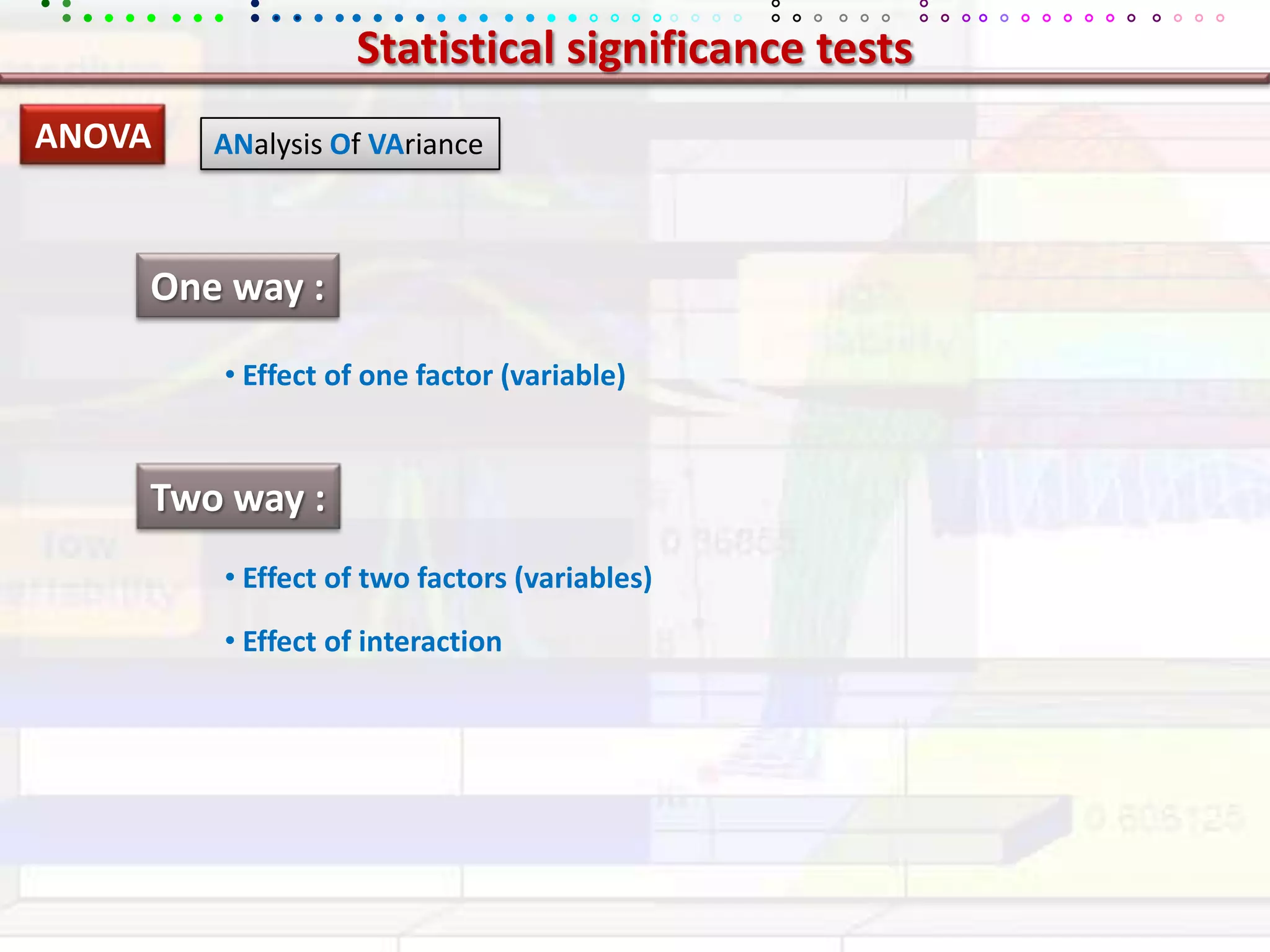
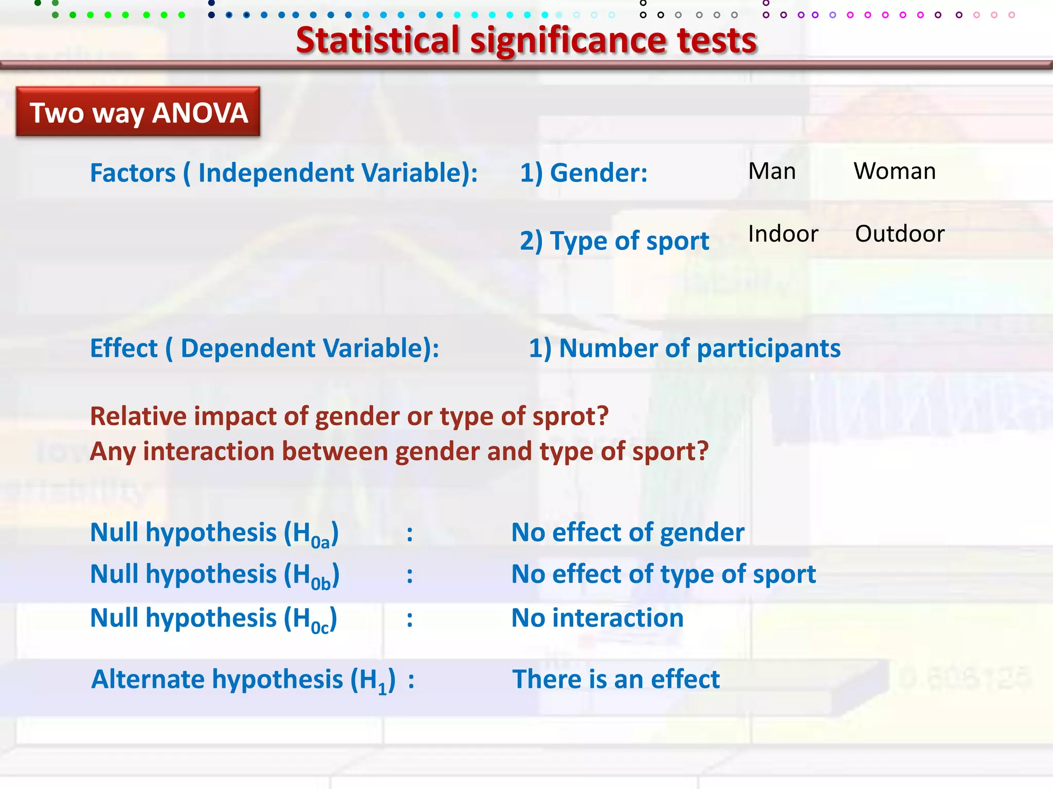
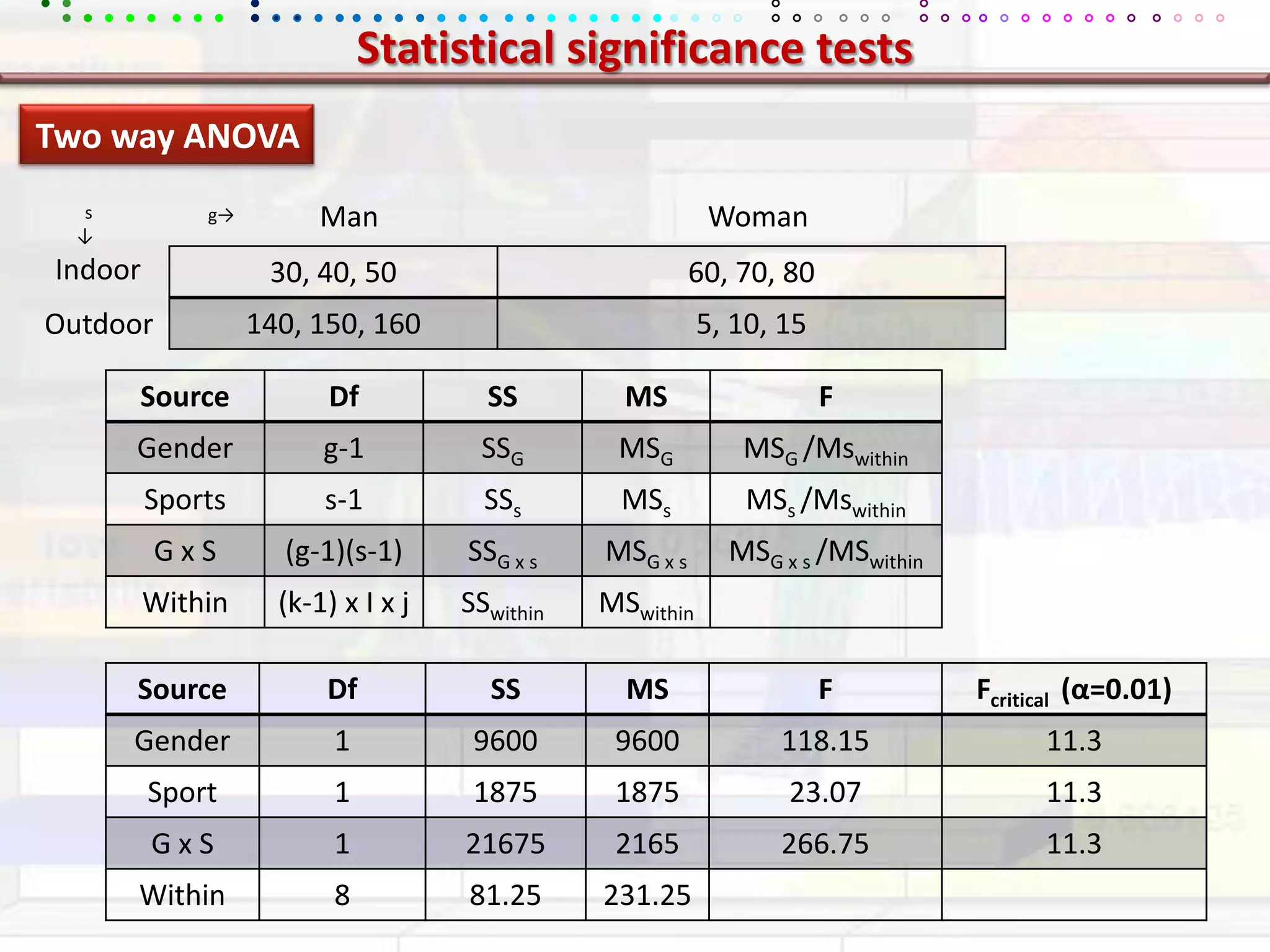
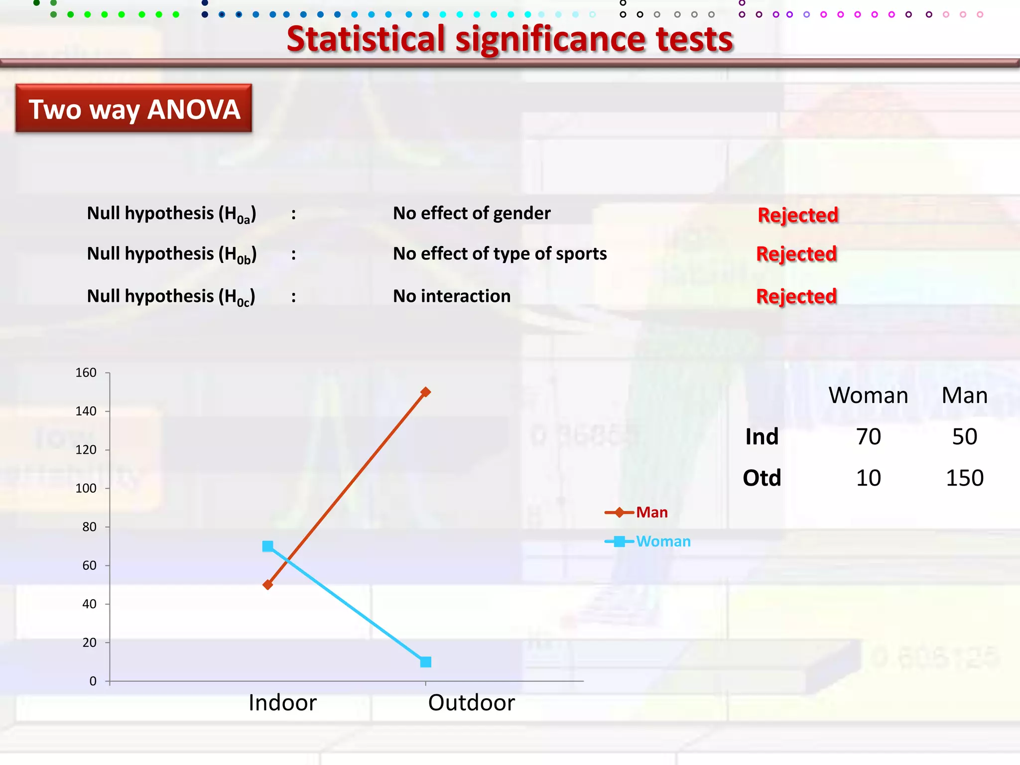
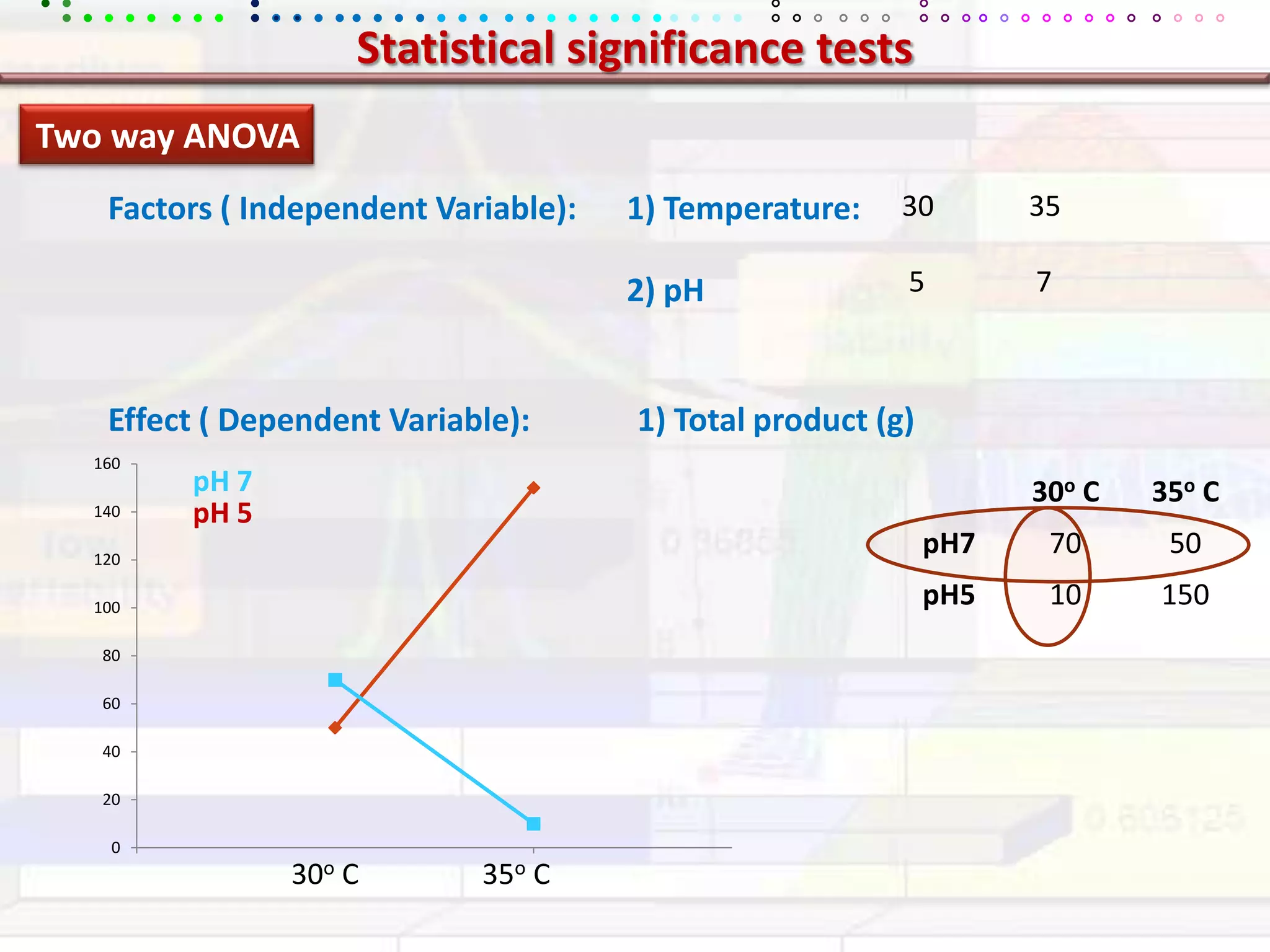
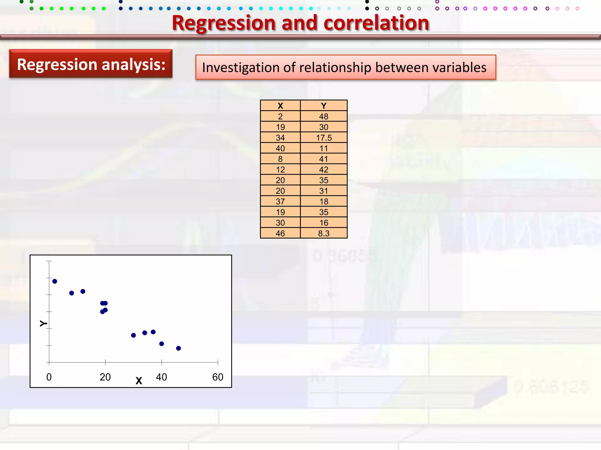
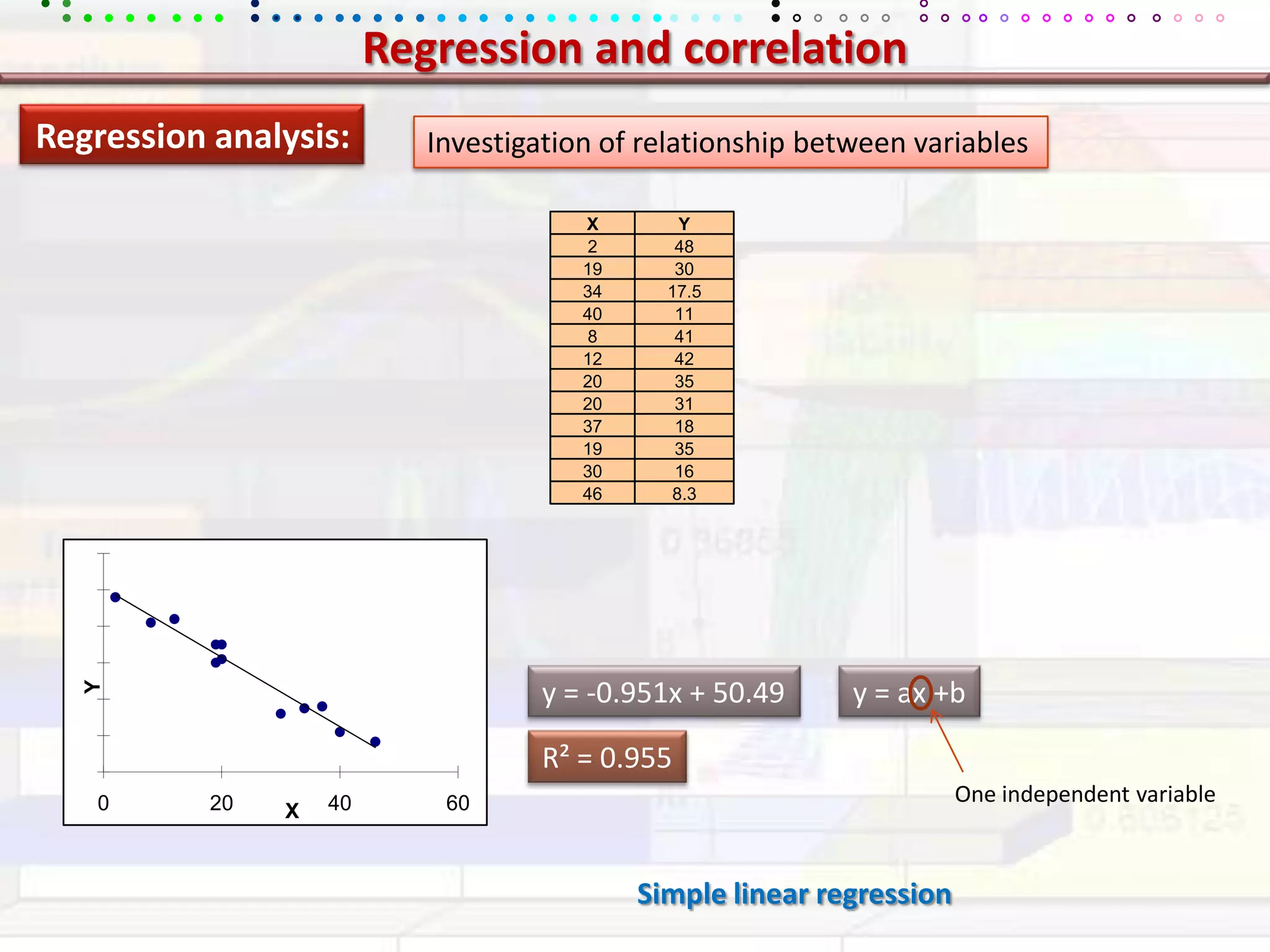
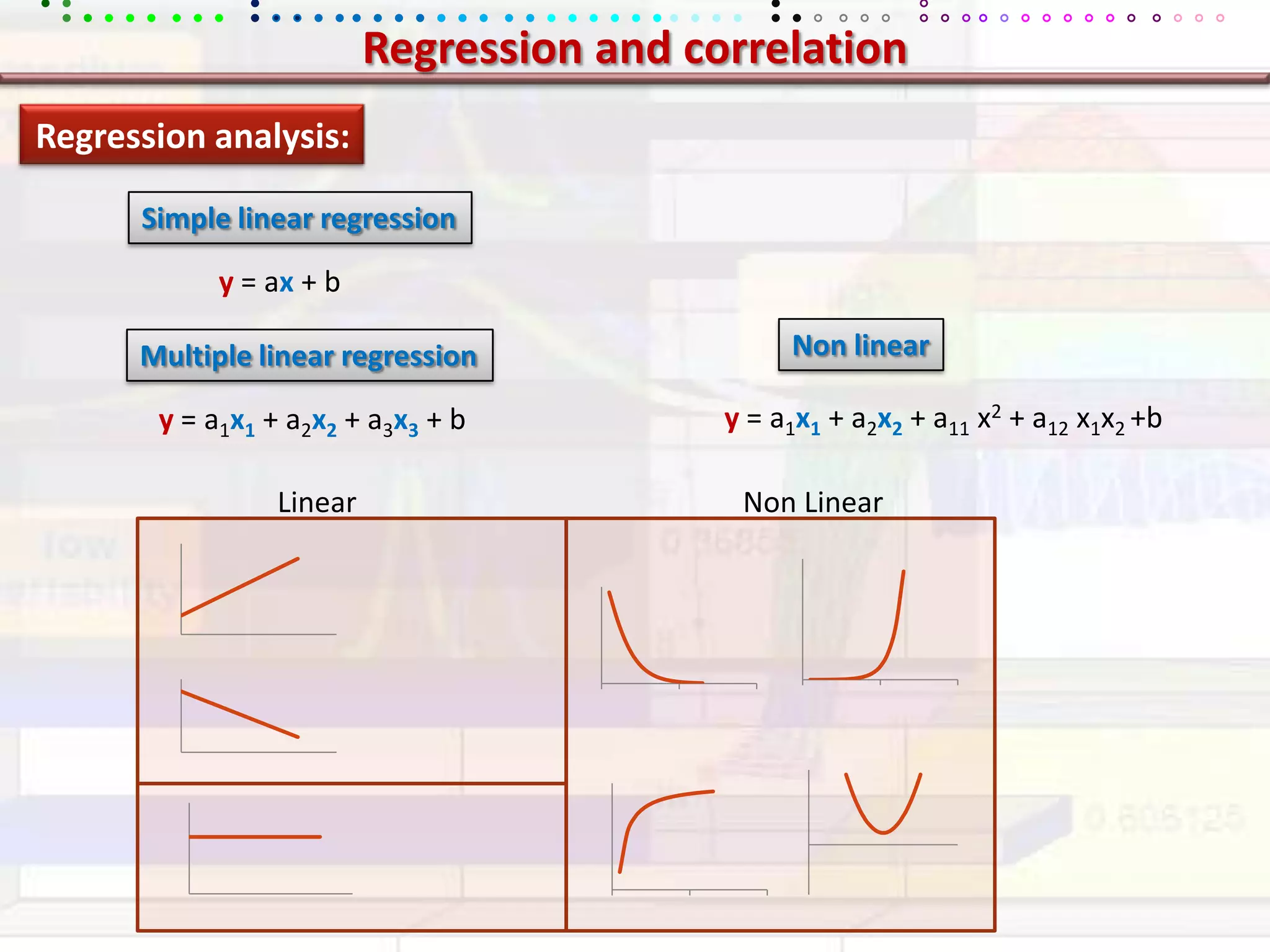
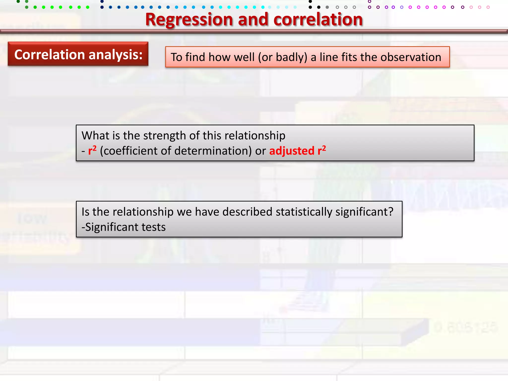
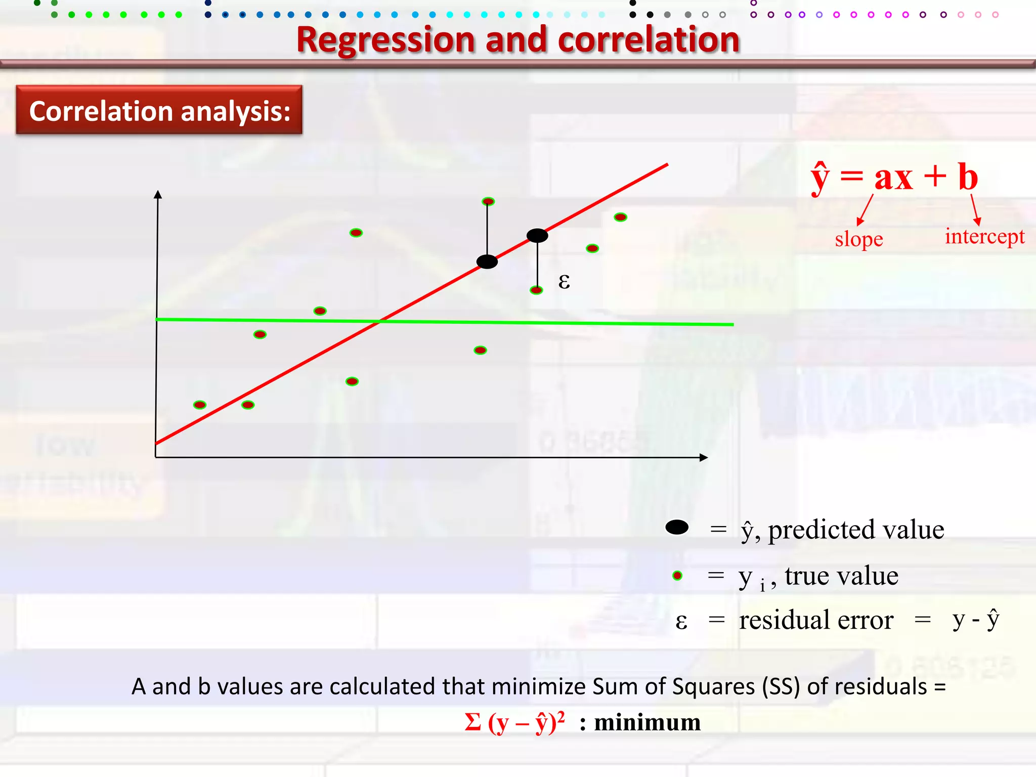
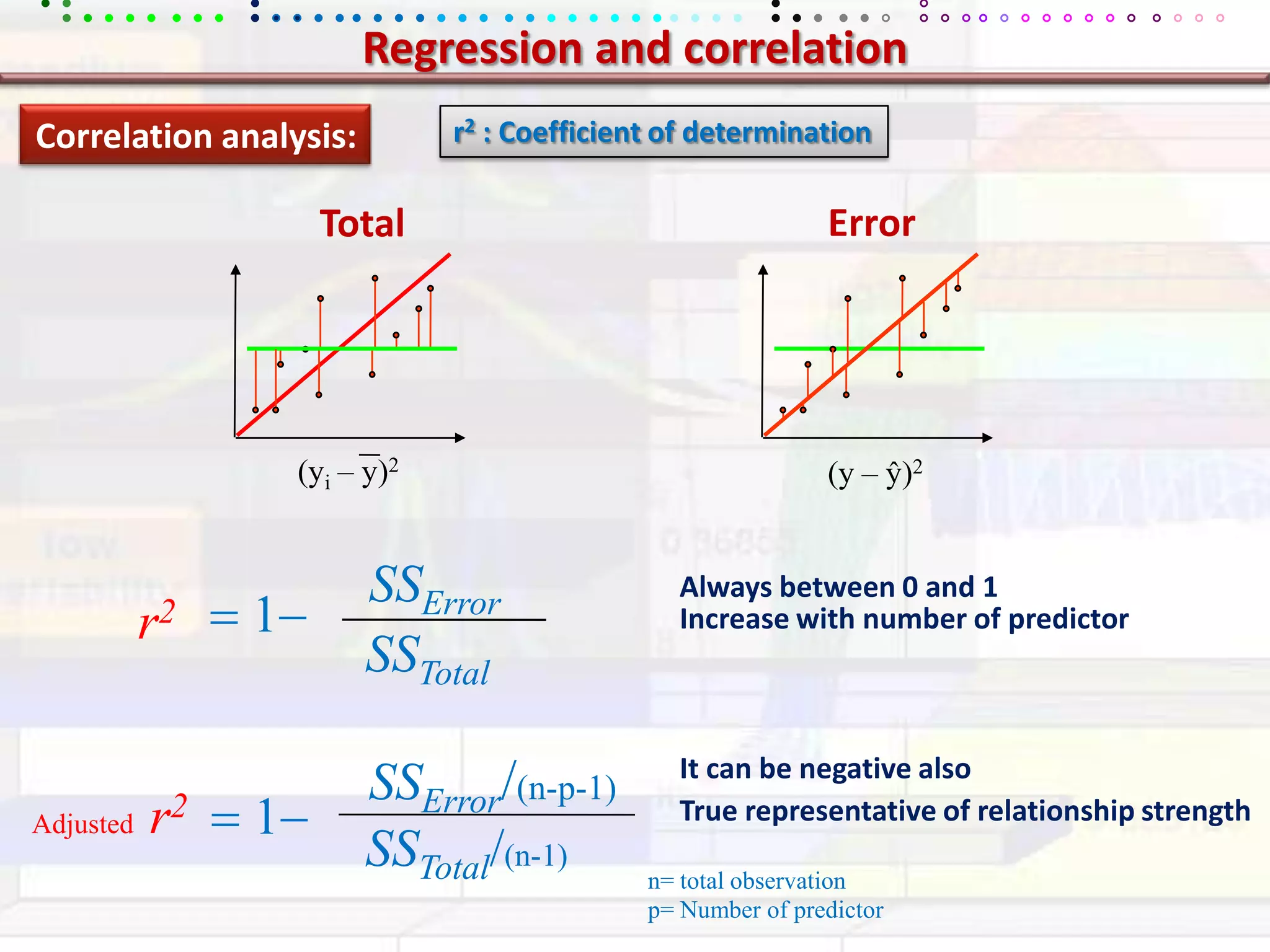
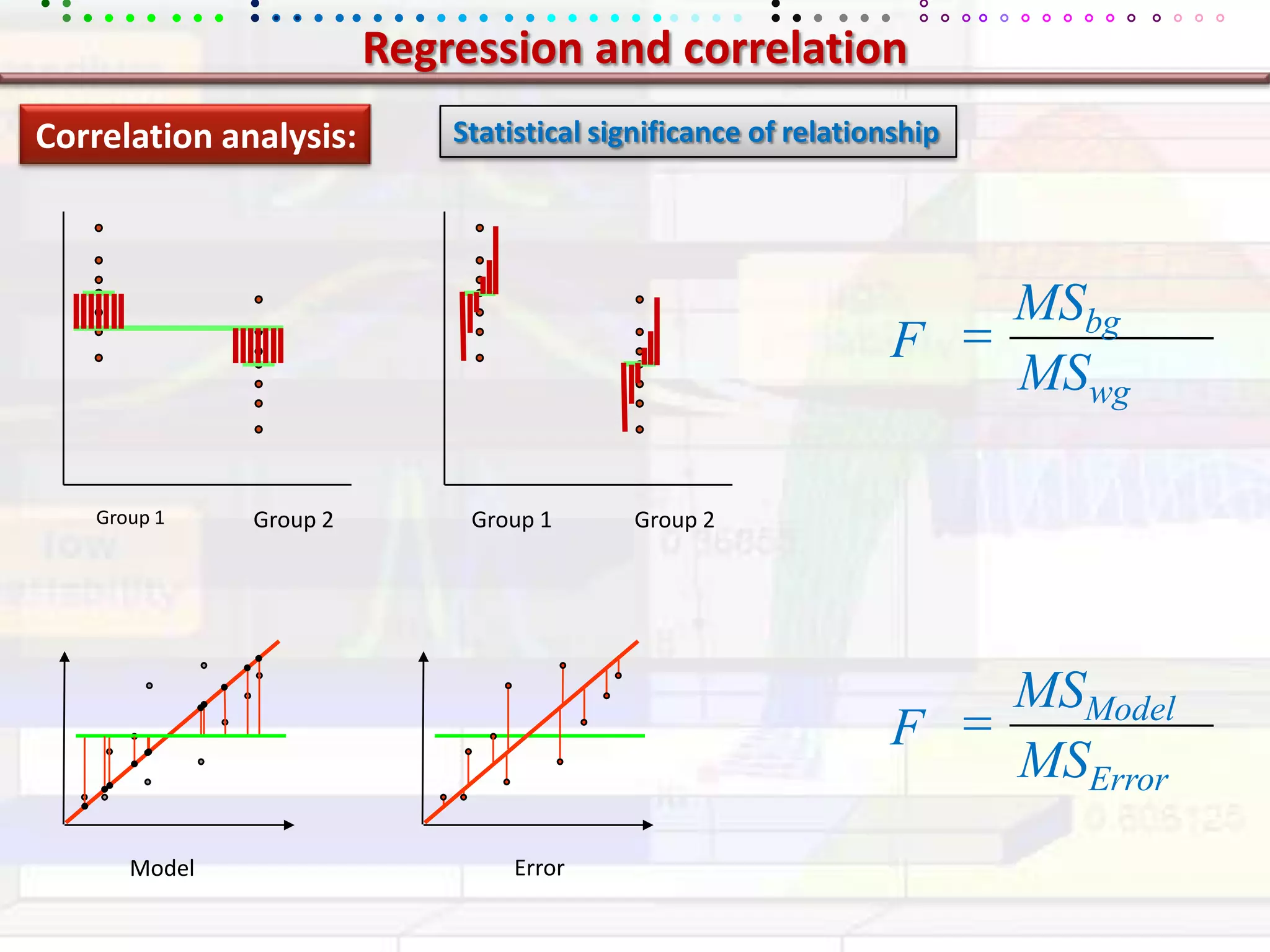
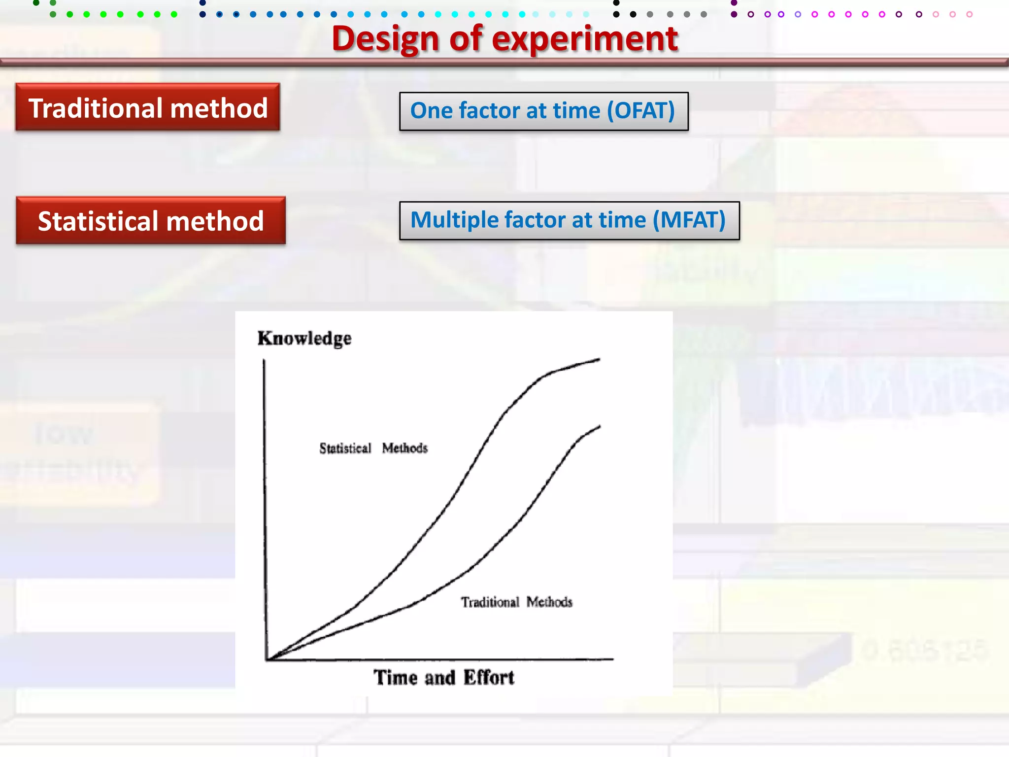
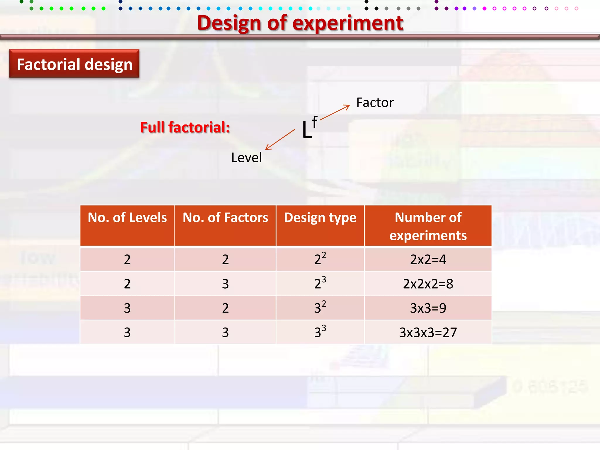
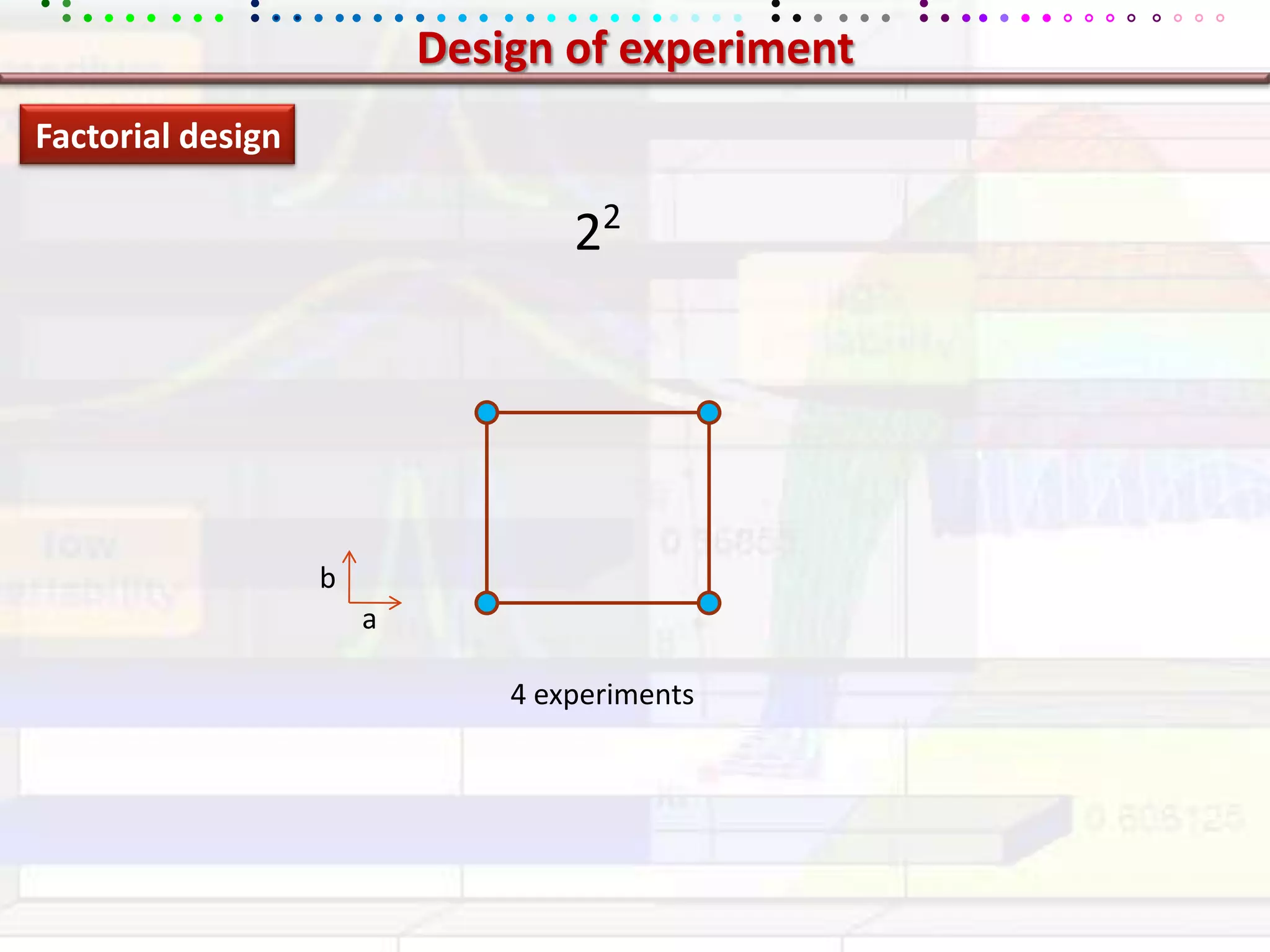
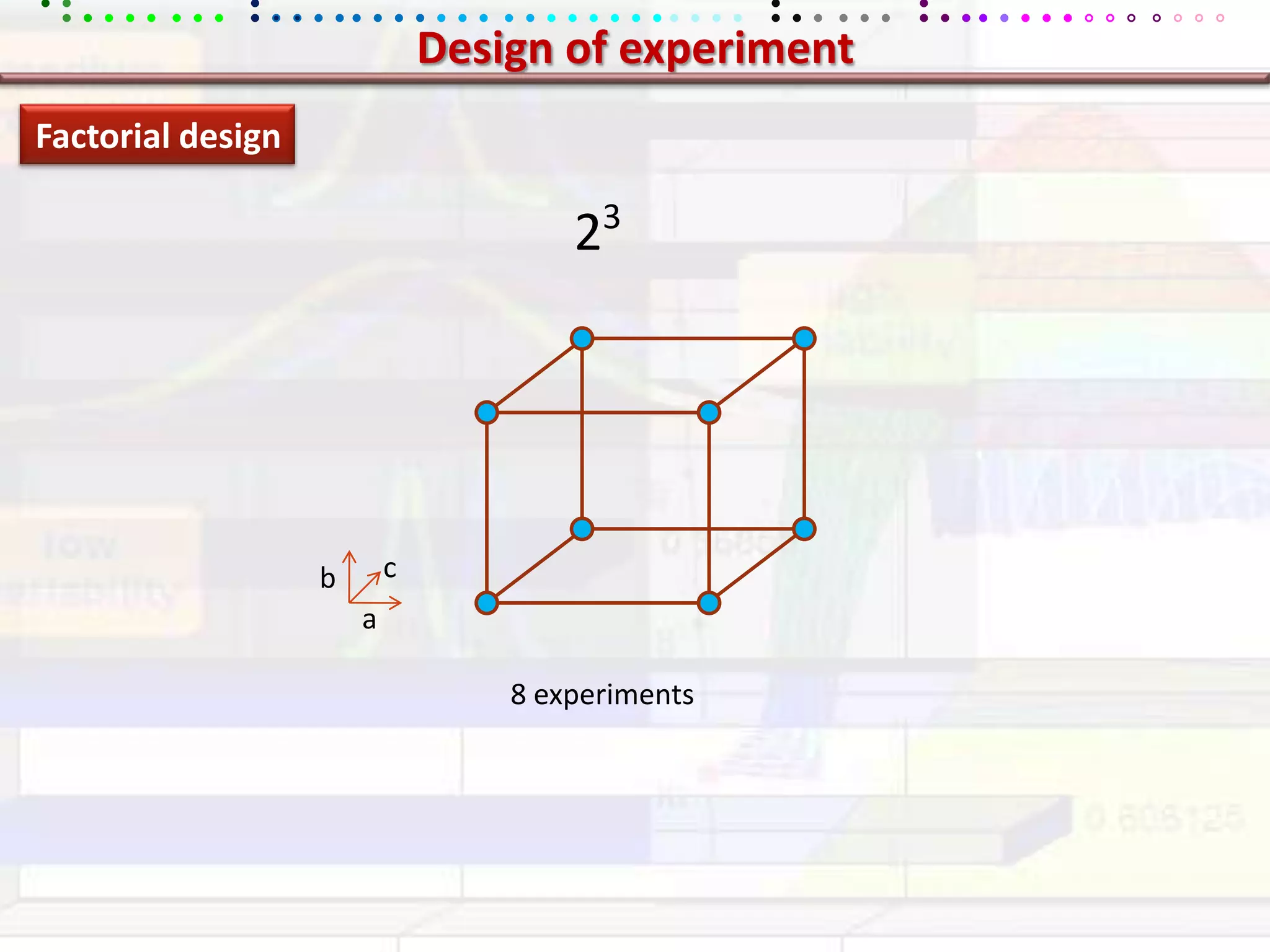
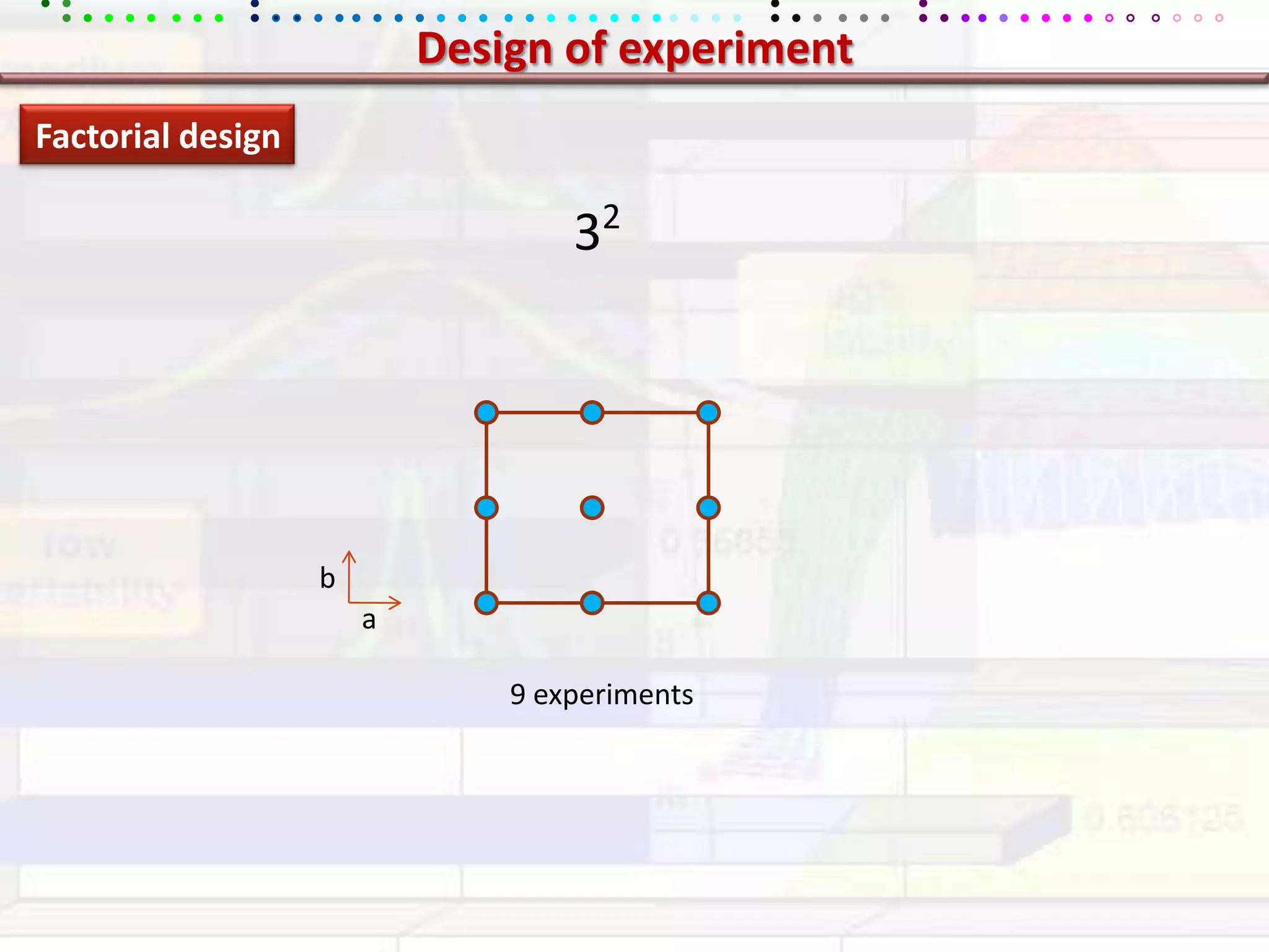
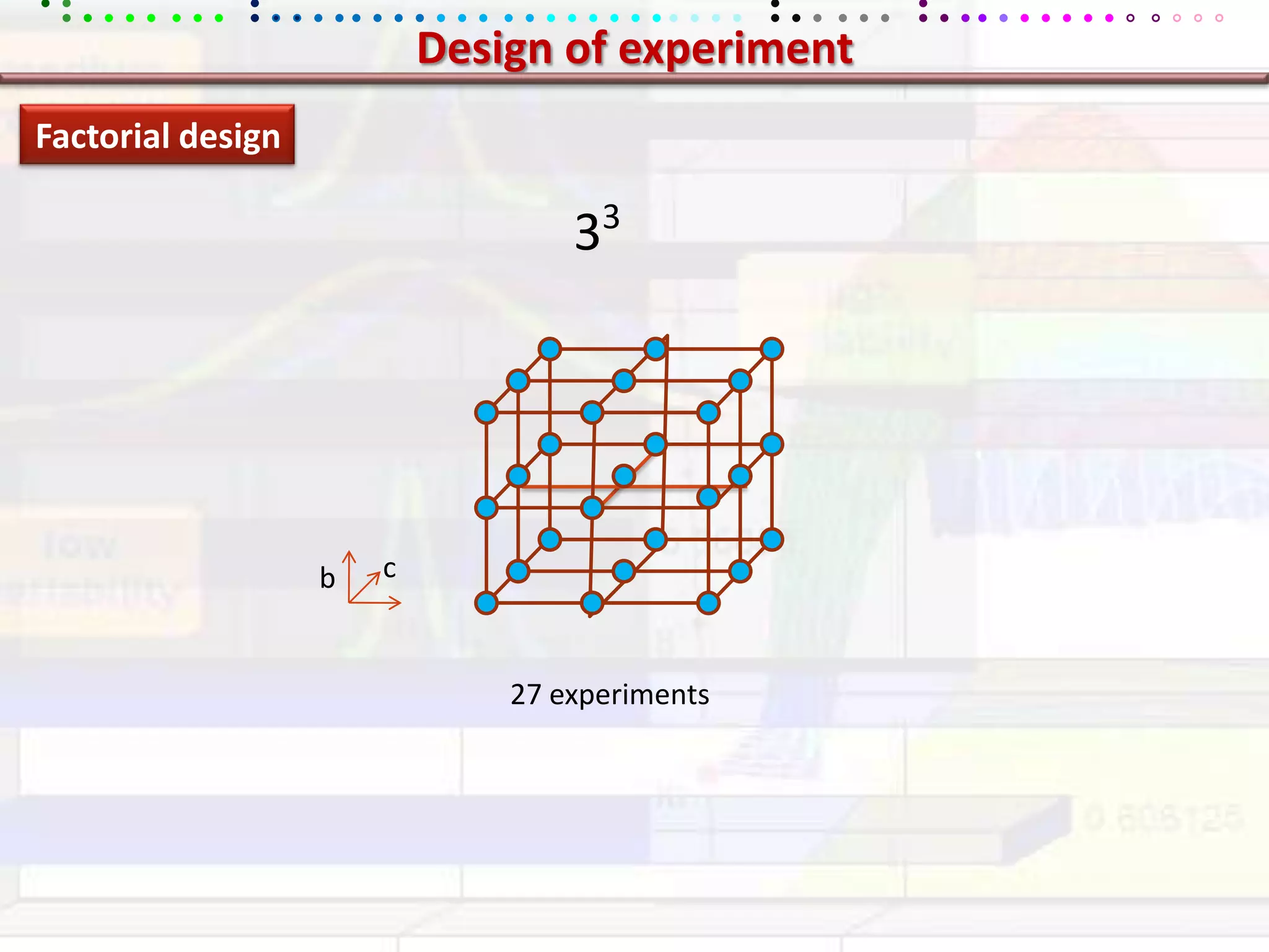
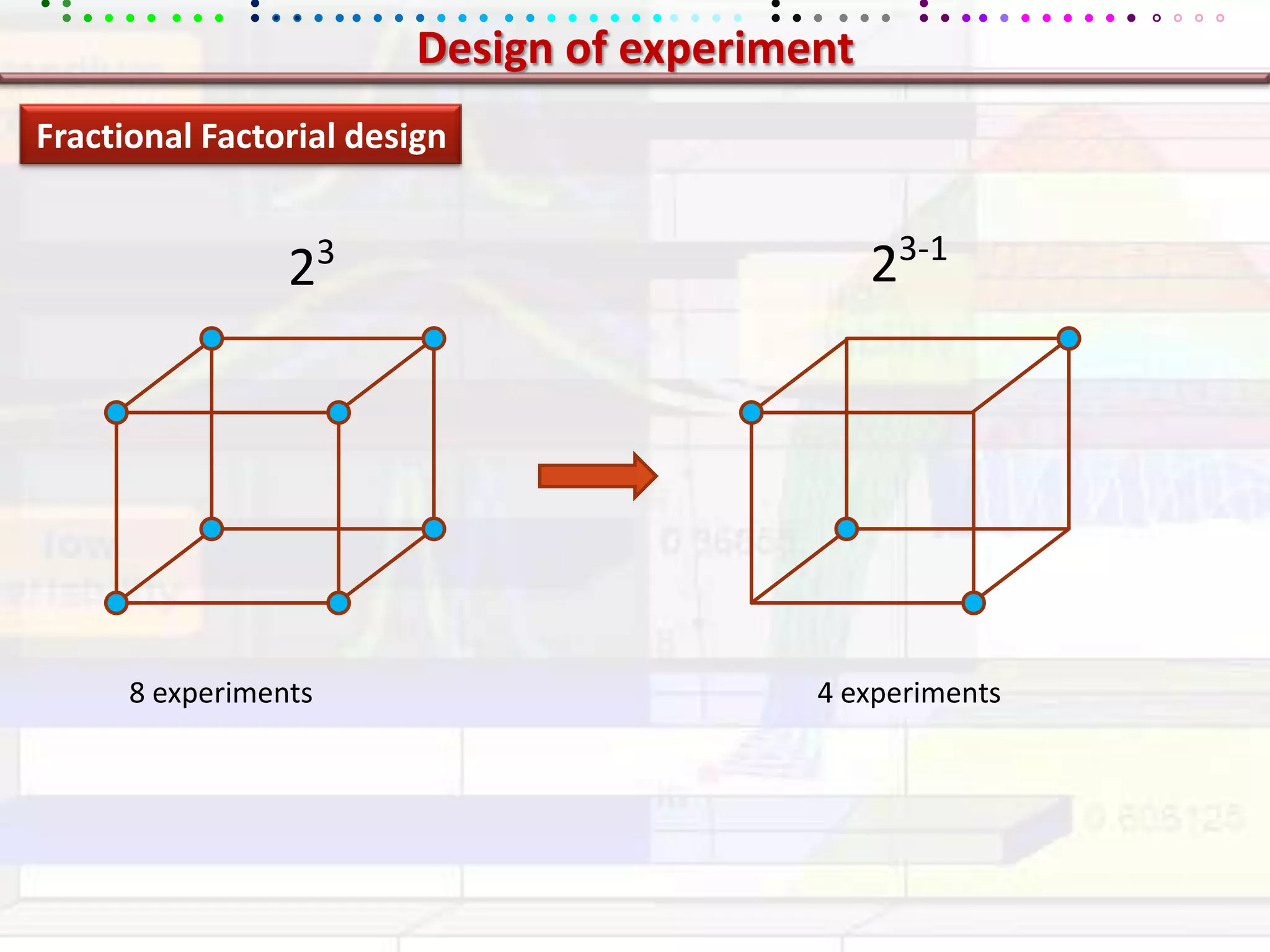
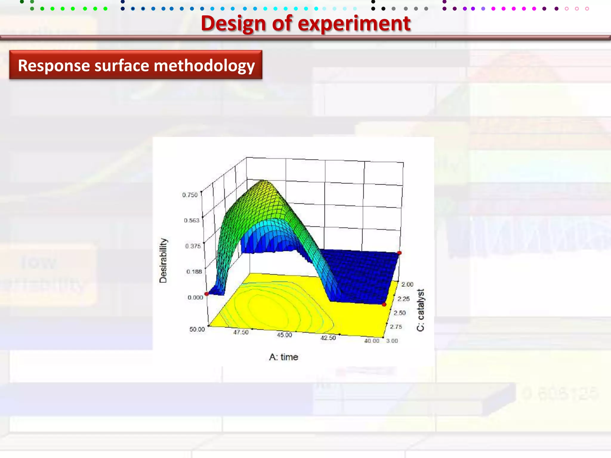
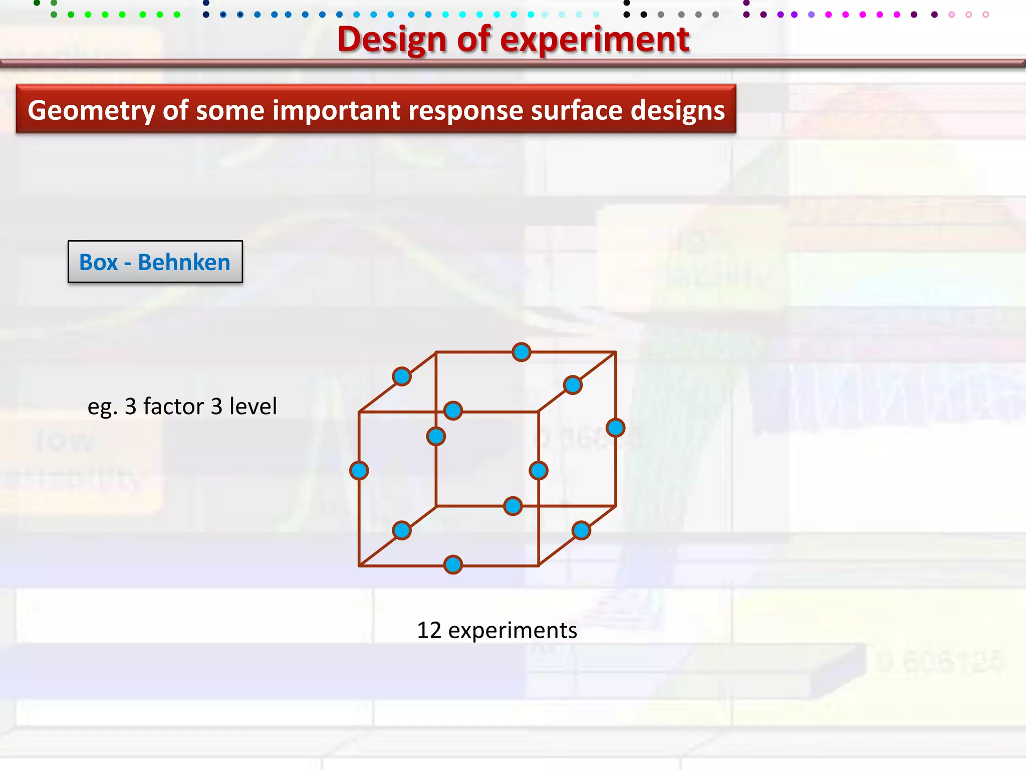
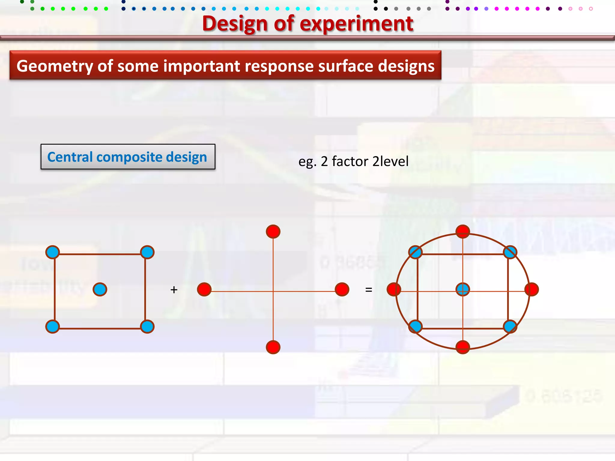
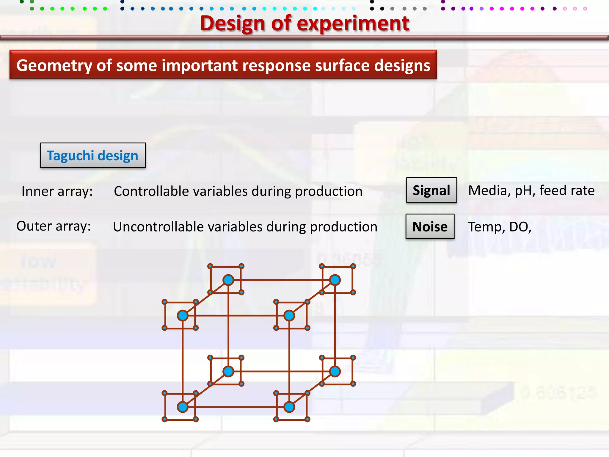
This document provides an overview of key concepts in applied statistics and design of experiments (DOE). It defines common measures of central tendency (mean, median, mode) and dispersion (variance, standard deviation, coefficient of variation). It also describes hypothesis testing using z-tests, t-tests, F-tests and ANOVA. Key concepts in regression, correlation and different experimental designs like factorial, fractional factorial and response surface methodology are summarized.

1. Applied Statistics and DOE Mayank

2. Applied Statistics Measures of central tendency (central position of data) µ Mean Population : Sample: Median Mode Measures of dispersion (spread of data) Variance σ2 s2 Population : Sample: Standard deviation σ s Population : Sample: Coefficient of variation

3. Measures of Central tendency Data: 34, 43, 81, 106, 106 and 115 Mean Average Σx/n =80.83 Mode Highest frequency =106 Median Middle score (81+106)/2 =93.5

4. Measures of dispersion Variance: Standard deviation: x SS SS/(n-1) MS sd √MS Most of the data lies between 44.5±4,57 = 39to 49

5. Measures of dispersion Coefficient of Variance CV = s/ *100% 4.57/44.5*100% = 10.28% Standard deviation is 10.28% of the mean

6. Measures of dispersion Normal Distribution Example: IQ Score

7. Measures of dispersion Normal Distribution IQ Score Count Score <55 115 130 145 100 85 70 55 145<

8. Measures of dispersion Normal Distribution 34.13% 34.13% Probability 13.59% 13.59 % Score 2.14% 2.14% 0.13% 0.13% 0.0031% 0.0031% 0.000028% 0.000028% Sd from -6σ -5σ -4σ -2σ -1σ 1σ 2σ 3σ -3σ 5σ 6σ 4σ μ 68.2689% 95.4499% 99.7300% 99.9936% 99.999942669% 99.999999802%

9. Measures of dispersion Normal Distribution Six Sigma DPMO DPHO LSL USL Sd from -6σ -5σ -4σ -2σ -1σ 1σ 2σ 3σ -3σ 5σ 6σ 4σ μ 99.999999802%

10. Measures of dispersion Normal Distribution LSL LSL USL USL

11. Measures of dispersion Normal Distribution 1.5 σ LSL USL 3.4 DMPO -6σ -5σ -4σ -2σ -1σ 1σ 2σ 3σ 4σ -3σ 5σ 6σ μ

12. Statistical significance tests Significance tests Z- test t- test F- test ANOVA

13. Statistical significance tests Z - test Z-value : How many standard deviations away from mean? +ve z: values are above the mean, -ve z: values are below the mean Population Sample Group compared to population 1 point compared to population

14. Statistical significance tests Z - test Sample : BMI Mean ( ) = 26.20 Standard deviation (s) = 6.57 What is the probability that of a person having BMI 19.2 sdbelow the mean 19.2 sd above the mean A person with a BMI of 19.2 has a z score of: So this person has a BMI 1.07 standard deviations below the mean

15. Statistical significance tests Z - test Sample : Probability <19.6 >19.6 Sd 16 % 84 % -1σ μ Standard deviation Z score 0 -1

16. Statistical significance tests Z - test Population : Test group : Employee having two wheeler Test : Commuting time from home to Biocon Claim : Average commuting time is less than 24 min At 0.01 level of significance (α=0.01): Is there enough evidence to support the research claim??? Samples : 30 18 16 23 19 25 48 13 17 20 23 16 21 18 16 29 15 8 19 20 7 15 16 24 15 6 11 14 23 18 12

17. Statistical significance tests Z - test Population : Assumption: Population is normally distributed Probability Score 24 Mean X

18. Statistical significance tests Z - test Population : Hypothesis testing Test vs Population Comparison of means: Null hypothesis : H0 No difference (Claim not true) H0 : x ≥ µ µ = 24 Alternate hypothesis : H1 It is different (Claim is true) H1 : x < µ

19. Statistical significance tests Z - test Population : Probability Probability 24 Mean X Z value Score Level of significance α = 0.01 Critical value Z 0 -2.33

20. Statistical significance tests Z - test Population : Ztest< Zcritical Ztest>Zcritical Rejection region Acceptance region -2.33 Z = 18.2 s = 7.7 Z = - 4.13 µ = 24 n = 30

21. Statistical significance tests Z - test Population : Rejection region -2.33 - 4.13 Z So is test value is significantly different (lower) than the mean Yes: There are significant evidence to reject the null hypothesis H0 : s ≥ 24 Rejected and therefore accept the claim H1 : s < 24 Significantly supported

22. Statistical significance tests t - test Comparison of means between two groups H0: H1: Null hypothesis will be rejected ttest > tcritical Null hypothesis will not be rejected ttest < tcritical

23. Statistical significance tests t - test Comparison of means between two groups Signal Difference between group means t = = Noise Variability of groups

24. Statistical significance tests t - test Effect of fertilizer on plant height Case 1 Fertilizer w/o Fertilizer 27.15 – 17.9 t test = = 2.4 t critical with 38 df at 0.05 significance level = 2.03 Plant height df = 2n-2 ttest > tcritical So is significantly different from H0: Rejected H1: s2

25. Statistical significance tests t - test Case 2 Fertilizer w/o Fertilizer t critical =2.03 1.3 t test = Plant height ttest < tcritical So is not significantly different from H0: Not rejected Rejected H1: s2

26. Statistical significance tests t - test Overview

27. Statistical significance tests F - test Comparison of variances where and are the sample variances F = The F hypothesis test is defined as: H0: = Rejected Ha: < > ≠ If Ftest > Fcritical (at significant level)

30. Statistical significance tests One way ANOVA Is there any impact of exam room temperature on student performance? Factor ( Independent Variable): Temperature (cold, optimum, hot) Effect ( Dependent Variable): Score (marks obtained) Null hypothesis (H0) : No effect (µ1= µ2 = µ3) Alternate hypothesis (H1) : There is an effect (µ1 ≠ µ2 ≠ µ3)

31. Statistical significance tests One way ANOVA C O H Cold Opt Hot Number of Attendees SS = X̄

32. Statistical significance tests One way ANOVA MSbg = = F = 6.40 MSwg Fcriticalfor Numerator degrees of freedom : 2 Denominator degrees of freedom : 33 At significance level (α) : 0.05 = 4.17 Ftest > Fcritical So there are enough evidence to reject null hypothesis H0: All means are same (no effect of Temperature) Rejected At 95% confidence level we can say: That the variation between means is not just by chance Examination Room temperature matters significantly

33. Statistical significance tests Two way ANOVA Factors ( Independent Variable): 1) Gender: Man Woman 2) Type of sport Indoor Outdoor Effect ( Dependent Variable): 1) Number of participants Relative impact of gender or type of sprot? Any interaction between gender and type of sport? Null hypothesis (H0a) : No effect of gender Null hypothesis (H0b) : No effect of type of sport Null hypothesis (H0c) : No interaction Alternate hypothesis (H1) : There is an effect

34. Statistical significance tests Two way ANOVA Man Woman s ↓ g-> Indoor Outdoor

35. Statistical significance tests Two way ANOVA Indoor Outdoor Null hypothesis (H0a) : No effect of gender Rejected Rejected Null hypothesis (H0b) : No effect of type of sports Rejected Null hypothesis (H0c) : No interaction

36. Statistical significance tests Two way ANOVA Factors ( Independent Variable): 1) Temperature: 30 35 2) pH 5 7 Effect ( Dependent Variable): 1) Total product (g) pH 7 pH 5 30o C 35o C

37. Regression and correlation Regression analysis: Investigation of relationship between variables

38. Regression and correlation Regression analysis: Investigation of relationship between variables y = -0.951x + 50.49 y = ax +b R² = 0.955 One independent variable Simple linear regression

39. Regression and correlation Regression analysis: Simple linear regression y = ax + b Non linear Multiple linear regression y = a1x1+ a2x2+ a11 x2 + a12 x1x2+b y = a1x1+ a2x2+ a3x3+ b Linear Non Linear

40. Regression and correlation Correlation analysis: To find how well (or badly) a line fits the observation What is the strength of this relationship - r2 (coefficient of determination) or adjusted r2 Is the relationship we have described statistically significant? -Significant tests

41. Regression and correlation Correlation analysis: ŷ = ax + b intercept slope ε = ŷ, predicted value = y i, true value ε =residual error = y - ŷ A and b values are calculated that minimize Sum of Squares (SS) of residuals = Σ (y – ŷ)2 : minimum

42. Regression and correlation Correlation analysis: r2 : Coefficient of determination Error Total (yi – y)2 (y – ŷ)2 Always between 0 and 1 Increase with number of predictor SSError = 1- r2 SSTotal It can be negative also SSError/(n-p-1) Adjusted r2 = 1- True representative of relationship strength SSTotal/(n-1) n= total observation p= Number of predictor

43. MSbg MSModel = = F F MSwg MSError Group 1 Group 1 Group 2 Group 2 Regression and correlation Correlation analysis: Statistical significance of relationship Error Model

44. Design of experiment Traditional method One factor at time (OFAT) Statistical method Multiple factor at time (MFAT)

45. Design of experiment

46. Design of experiment How to select a design?

47. Design of experiment- terminology Independent variable/s Factors Continuous Numeric: any value between lower and upper value eg. Temperature, pH, concentration Categorical Numeric/non-numeric : only characters or levels eg. Gender, operator, type, temperature Levels -1(lower) +1(higher) 0(middle) Range of a factor/s Effects Dependent variable/s: Response Main effect/s Effect/s due to individual factor/s Interaction effect/s Effect/s due to interaction of multiple factors Confounding/Aliasing When two or more effects can not be distinguished eg. Main effect is confounded with interaction effects Main effects and interaction effects are aliased

48. Design of experiment Resolution of a design Power of a design Higher order interaction are less significant than lower order interaction

49. Design of experiment Factorial design Factor Lf Full factorial: Level

50. Design of experiment Factorial design 22 b a 4 experiments

51. Design of experiment Factorial design 23 c b a 8 experiments

52. Design of experiment Factorial design 32 b a 9 experiments

53. Design of experiment Factorial design 33 c b 27 experiments

54. Design of experiment Fractional Factorial design 23-1 23 8 experiments 4 experiments

55. Design of experiment Response surface methodology

56. Design of experiment Geometry of some important response surface designs Box - Behnken eg. 3 factor 3 level 12 experiments

57. Design of experiment Geometry of some important response surface designs Central composite design eg. 2 factor 2level + =

58. Design of experiment Geometry of some important response surface designs Taguchi design Signal Media, pH, feed rate Inner array: Controllable variables during production Outer array: Uncontrollable variables during production Noise Temp, DO,