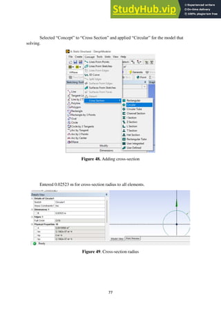
Downloaded 12 times


![22
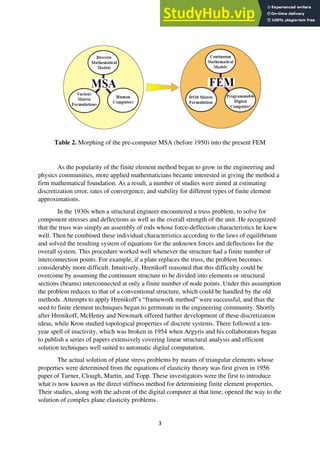
1.4. MATRIX ALGEBRA FOR FINITE ELEMENT METHOD
These steps include discretizing the problem into elements and nodes, assuming a
function that represents behavior of an element, developing a set of equations for an
element, assembling the elemental formulations to present the entire problem, and
applying the boundary conditions and loading. These steps lead to a set of linear
(nonlinear for some problems) algebraic equations that must be solved simultaneously. A
good understanding of matrix algebra is essential in formulation and solution of finite
element models. As is the case with any topic, matrix algebra has its own terminology and
follows a set of rules.
1.4.1. Basic Definitions
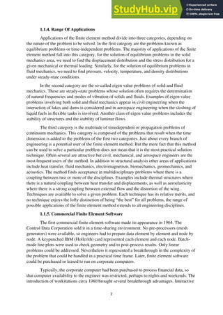
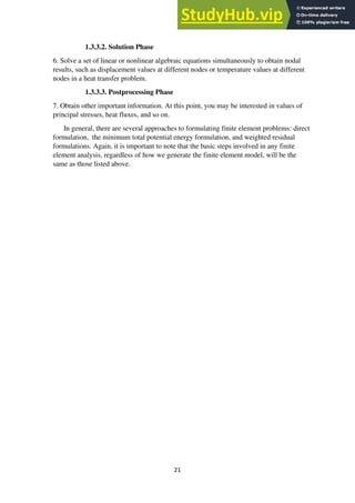
A matrix is an array of numbers or mathematical terms. The numbers or the
mathematical terms that make up the matrix are called the elements of matrix. The size of
a matrix is defined by its number of rows and columns. A matrix may consist of m rows
and n columns. For example,
Matrix [N] is a 3 by 3 matrix whose elements are numbers, [T] is a 4 x 4 that has sine
and cosine terms as its elements, {L} is a 3 x 1 matrix with its elements representing
partial derivatives, and [I] is a 2 x 2 matrix with integrals for its elements. The [N], [T],
and [I] are square matrices. A square matrix has the same number of rows and columns.
The element of a matrix is denoted by its location.
1.4.2. Column Matrix and Row Matrix
A column matrix is defined as a matrix that has one column but could have many
rows. On the other hand, a row matrix is a matrix that has one row but could have many
columns. Examples of column and row matrices follow.](https://image.slidesharecdn.com/analysisofatrussusingfiniteelementmethods-230804175539-9cf69e62/85/ANALYSIS-OF-A-TRUSS-USING-FINITE-ELEMENT-METHODS-33-320.jpg)
![24
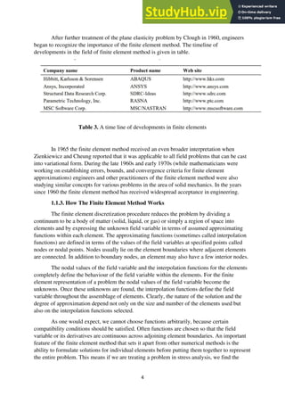
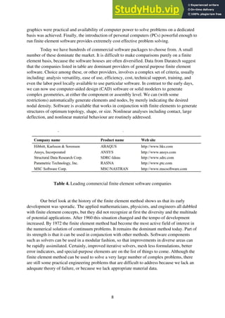
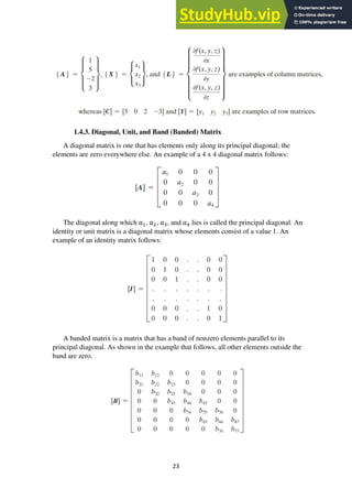
1.4.4. Upper and Lower Triangular Matrix
An upper triangular matrix is one that has zero elements below the principal diagonal,
and the lower triangular matrix is one that has zero elements above the principal diagonal.
Examples of upper triangular and lower triangular matrices are shown below.
1.4.5. Matrix Addition or Subtraction
Two matrices can be added together or subtracted from each other provided that
they are of the same size each matrix must have the same number of rows and columns.
We can add matrix [A]m x n of dimension m by n to matrix [B]m x n of the same
dimension by adding the like elements. Matrix subtraction follows a similar rule, as
shown.
The rule for matrix addition or subtraction can be generalized in the following manner.
Let us denote the elements of matrix [A] by 𝑎𝑖𝑗 and the elements of matrix [B] by 𝑏𝑖𝑗,
where the number of rows i varies from 1 to m and the number of columns j varies from 1
to n. If we were to add matrix [A] to matrix [B] and denote the resulting matrix by [C], it
follows that](https://image.slidesharecdn.com/analysisofatrussusingfiniteelementmethods-230804175539-9cf69e62/85/ANALYSIS-OF-A-TRUSS-USING-FINITE-ELEMENT-METHODS-35-320.jpg)
![25
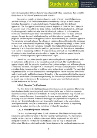
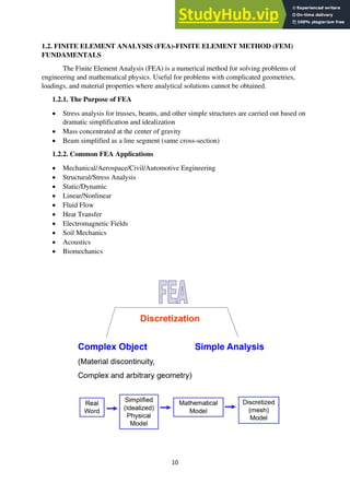
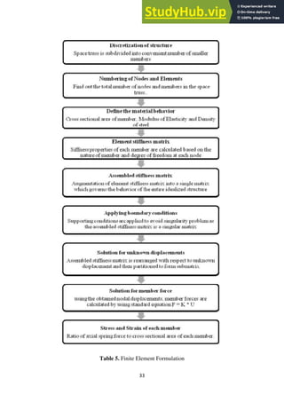
1.4.6. Matrix Multiplication
1.4.6.1. Multiplying a Matrix by a Scalar Quantity
When a matrix [A] of size m x n is multiplied by a scalar quantity such as b, the
operation results in a matrix of the same size m x n, whose elements are the product of
elements in the original matrix and the scalar quantity. For example, when we multiply
matrix [A] of size m x n by a scalar quantity b, this operation results in another matrix of
size m x n, whose elements are computed by multiplying each element of matrix [A] by b,
as shown below.
1.4.6.2. Multiplying a Matrix by Another Matrix
Whereas any size matrix can be multiplied by a scalar quantity, matrix multiplication
can be performed only when the number of columns in the premultiplier matrix is equal to
the number of rows in the postmultiplier matrix. For example, matrix [A] of size m x n
can be premultiplied by matrix [B] of size n x p because the number of columns n in
matrix [A] is equal to number of rows n in matrix [B]. Moreover, the multiplication results
in another matrix, say [C], of size m x p. Matrix multiplication is carried out according to
the following rule:
where the elements in the first column of the [C] matrix are computed from](https://image.slidesharecdn.com/analysisofatrussusingfiniteelementmethods-230804175539-9cf69e62/85/ANALYSIS-OF-A-TRUSS-USING-FINITE-ELEMENT-METHODS-36-320.jpg)
![26
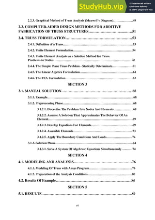
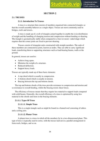
and the elements in the second column of the [C] matrix are
and similarly, the elements in the other columns are computed, leading to the last column
of the [C] matrix
The multiplication procedure that leads to the values of the elements in the [C] matrix may
be represented in a compact summation form by
When multiplying matrices, keep in mind the following rules. Matrix multiplication is not
commutative except for very special cases.
[A][B] ≠ [B][A]
Matrix multiplication is associative; that is
[A]([B][C]) = ([A][B])[C]
The distributive law holds true for matrix multiplication; that is
([A] + [B])[C] = [A][C] + [B][C]
Or
[A]([B] + [C]) = [A][B] + [A][C]
For a square matrix, the matrix may be raised to an integer power n in the following
manner:
This may be a good place to point out that if [I] is an identity matrix and [A] is a square
matrix of matching size, then it can be readily shown that the product of
[I][ A] = [A][ I] = [A].](https://image.slidesharecdn.com/analysisofatrussusingfiniteelementmethods-230804175539-9cf69e62/85/ANALYSIS-OF-A-TRUSS-USING-FINITE-ELEMENT-METHODS-37-320.jpg)
![27
1.4.6.3. Partitioning of a Matrix
Finite element formulation of complex problems typically involves relatively large
sized matrices. For these situations, when performing numerical analysis dealing with
matrix operations, it may be advantageous to partition the matrix and deal with a subset of
elements. The partitioned matrices require less computer memory to perform the
operations. Traditionally, dashed horizontal and vertical lines are used to show how a
matrix is partitioned. For example, we may partition matrix [A] into four smaller matrices
in the following manner:
It is important to note that matrix [A] could have been partitioned in a number of other
ways, and the way a matrix is partitioned would define the size of submatrices.
1.4.6.4. Addition and Subtraction Operations Using Partitioned Matrices
Now let us turn our attention to matrix operations dealing with addition, subtraction,
or multiplication of two matrices that are partitioned. Consider matrix [B] having the same
size (5 x 6) as matrix [A]. If we partition matrix [B] in exactly the same way we
partitioned [A] previously, then we can add the submatrices in the following manner:](https://image.slidesharecdn.com/analysisofatrussusingfiniteelementmethods-230804175539-9cf69e62/85/ANALYSIS-OF-A-TRUSS-USING-FINITE-ELEMENT-METHODS-38-320.jpg)
![28
Where
Then, using submatrices we can write,
1.4.6.5. Matrix Multiplication Using Partitioned Matrices
As mentioned earlier, matrix multiplication can be performed only when the number
of columns in the premultiplier matrix is equal to the number of rows in the postmultiplier
matrix. Referring to [A] and [B] matrices of the preceding section, because the number of
columns in matrix [A] does not match the number of rows of matrix [B], then matrix [B]
cannot be premultiplied by matrix [A]. To demonstrate matrix multiplication using
submatrices, consider matrix [C] of size 6 x 3, which is partitioned in the manner shown
below.
Where,](https://image.slidesharecdn.com/analysisofatrussusingfiniteelementmethods-230804175539-9cf69e62/85/ANALYSIS-OF-A-TRUSS-USING-FINITE-ELEMENT-METHODS-39-320.jpg)
![29
Next, consider premultiplying matrix [C] by matrix [A]. Let us refer to the results of
this multiplication by matrix [D] of size 5 x 3. In addition to paying attention to the size
requirement for matrix multiplication, to carry out the multiplication using partitioned
matrices, the premultiplying and postmultiplying matrices must be partitioned in such a
way that the resulting submatrices conform to the multiplication rule. That is, if we
partition matrix [A] between the third and the fourth columns, then matrix [C] must be
partitioned between the third and the fourth rows. However, the column partitioning of
matrix [C] may be done arbitrarily, because regardless of how the columns are partitioned,
the resulting submatrices will still conform to the multiplication rule. In other words,
instead of partitioning matrix [C] between columns two and three, we could have
partitioned the matrix between columns one and two and still carried out the
multiplication using the resulting submatrices.
1.4.7. Transpose of a Matrix
The finite element formulation lends itself to situations wherein it is desirable to
rearrange the rows of a matrix into the columns of another matrix. Which is shown here
again for the sake of continuity and convenience.
and its position in the global matrix,
Instead of putting together [K] (1G) by inspection as we did, we could obtain [K] (1G)
using the following procedure:](https://image.slidesharecdn.com/analysisofatrussusingfiniteelementmethods-230804175539-9cf69e62/85/ANALYSIS-OF-A-TRUSS-USING-FINITE-ELEMENT-METHODS-40-320.jpg)
![30
Where,
[𝐴1] T, called the transpose of [𝐴1], is obtained by taking the first and the second rows of
[𝐴1] and making them into the first and the second columns of the transpose matrix. It is
easily verified that by carrying out the multiplication, we will arrive at the same result that
was obtained by inspection.
Similarly, we could have performed the following operation to obtain [𝐾](2𝐺)
:](https://image.slidesharecdn.com/analysisofatrussusingfiniteelementmethods-230804175539-9cf69e62/85/ANALYSIS-OF-A-TRUSS-USING-FINITE-ELEMENT-METHODS-41-320.jpg)
![31
As you have seen from the previous examples, we can use a positioning matrix, such
as [A] and its transpose, and methodically create the global stiffness matrix for finite
element models.
In general, to obtain the transpose of a matrix [B] of size m x n, the first row of the
given matrix becomes the first column of the [B] T, the second row of [B] becomes the
second column of [B] T, and so on, leading to the mth row of [B] becoming the mth
column of the [B] T, resulting in a matrix with the size of n x m. Clearly, if you take the
transpose of [B] T, you will end up with [B]. That is,
We write the solution matrices, which are column matrices, as row matrices using the
transpose of the solution another use for transpose of a matrix. For example, we represent
the displacement solution
When performing matrix operations dealing with transpose of matrices, the following
identities are true:
This is a good place to define a symmetric matrix. A symmetric matrix is a square
matrix whose elements are symmetrical with respect to its principal diagonal.
Note that for a symmetric matrix, element amn is equal to anm. That is, amn = anm for
all values of n and m. Therefore, for a symmetric matrix, [A] = [A] T.](https://image.slidesharecdn.com/analysisofatrussusingfiniteelementmethods-230804175539-9cf69e62/85/ANALYSIS-OF-A-TRUSS-USING-FINITE-ELEMENT-METHODS-42-320.jpg)

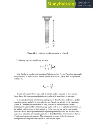
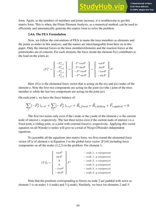
![57
{U} and {u} represent the displacements of nodes i and j with respect to the global XY
and the local xy frame of references, respectively. [T] is the transformation matrix that allows
for the transfer of local deformations to their respective global values. In a similar way, the
local and global forces may be related according to the equations
or, in matrix form,
Where,
are components of forces acting at nodes i and j with respect to global coordinates, and
represent the local components of the forces at nodes i and j.
A general relationship between the local and the global properties was derived in the
preceding steps. However, we need to keep in mind that for a given member the forces in
the local y-direction are zero. This fact is simply because under the two-force assumption,
a member can only be stretched or shortened along its longitudinal axis (local x-axis).](https://image.slidesharecdn.com/analysisofatrussusingfiniteelementmethods-230804175539-9cf69e62/85/ANALYSIS-OF-A-TRUSS-USING-FINITE-ELEMENT-METHODS-68-320.jpg)
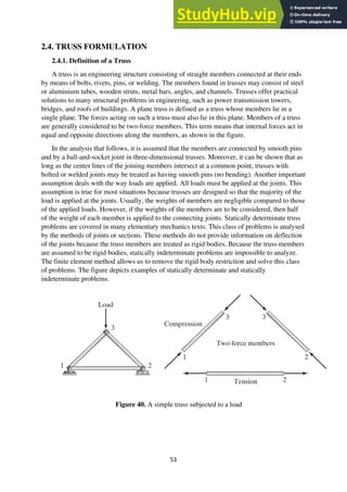
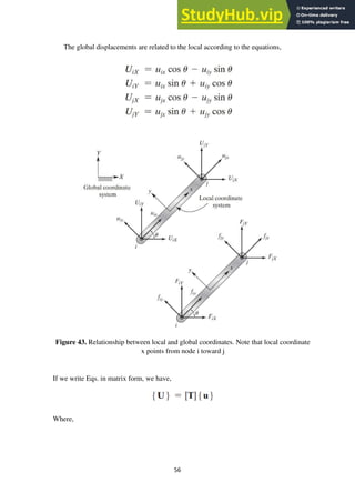
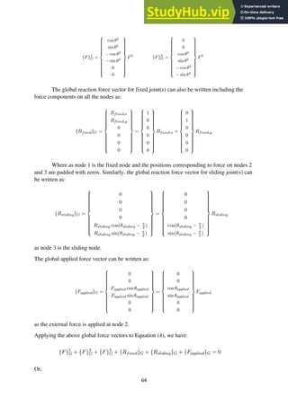
![59
In the figure Internal forces for an arbitrary truss element. Note that the static equilibrium
conditions require that the sum of fix and fjx be zero. Also note that the sum of fix and fjx
is zero regardless of which representation is selected.
The inverse of the transformation matrix [T] and is,
Multiplying both sides of Eq. by [T] and simplifying, we obtain,
Substituting for values of the [T], [k], [𝑇]−1
, and {U} matrices in Eq. and multiplying, we
are left with,](https://image.slidesharecdn.com/analysisofatrussusingfiniteelementmethods-230804175539-9cf69e62/85/ANALYSIS-OF-A-TRUSS-USING-FINITE-ELEMENT-METHODS-70-320.jpg)
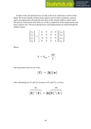
![60
The equations express the relationship between the applied forces, the element stiffness
matrix [𝑘]ⅇ
, and the global deflection of the nodes of an arbitrary element. The stiffness
matrix [𝑘]ⅇ
for any member (element) of the truss is,](https://image.slidesharecdn.com/analysisofatrussusingfiniteelementmethods-230804175539-9cf69e62/85/ANALYSIS-OF-A-TRUSS-USING-FINITE-ELEMENT-METHODS-71-320.jpg)
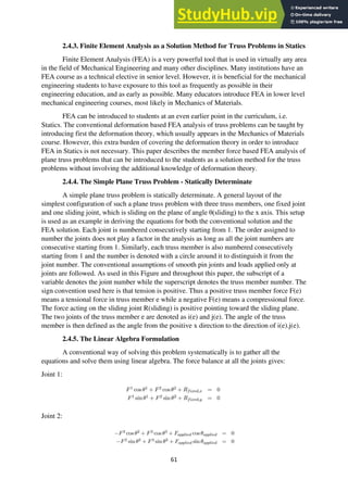
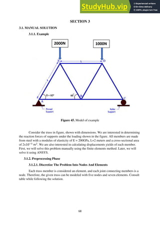
![62
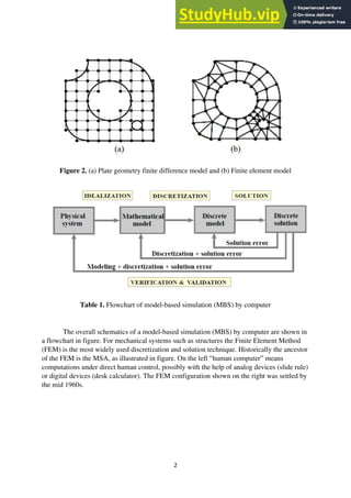
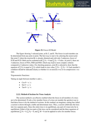
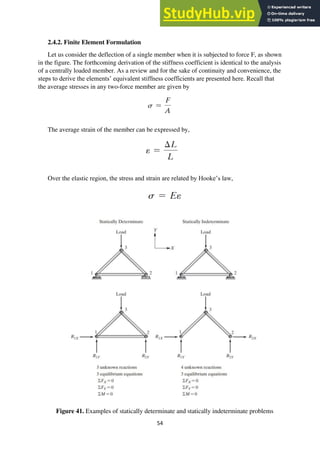
Figure 44. (a). A simple truss structure layout and forces on the joints/nodes (b). Notation and
forces on a truss member/element
Joint 3:
We have 6 equations for this problem and also 6 unknowns to solve for: three truss
member forces F(1),F(2),F(3), two fixed joint reaction forces R(fixed,x), R(fixed,y) y and one
sliding joint reaction force R(sliding), which is normal to the sliding plane. Moving the
known quantities to the right hand side of the equations and putting the equations into matrix
form yields:
Where as [K] is the coefficient matrix, {FR} is the unknown reaction force vector and
{FA} is the applied force vector from this simple linear algebra formulation. The solution is
then simply:
When a simple plane truss problem has more members and joints, two force balance
equations are written for each joint, and then all the equations are assembled into the matrix](https://image.slidesharecdn.com/analysisofatrussusingfiniteelementmethods-230804175539-9cf69e62/85/ANALYSIS-OF-A-TRUSS-USING-FINITE-ELEMENT-METHODS-73-320.jpg)
![65
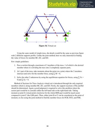
Simplifying and moving the known applied force vector to the right side of the equation, we
have:
which is exactly the same as Equation (1) from the direct linear algebra formulation. A close
examination of the Equation (12) yields that by arranging the unknown reaction force vector
as:
the coefficient matrix [K] of the final system of equations has the following properties:
• The first N(elem) columns correspond to the global force vectors of the N(elem) elements,
without the truss member forces as they are the unknowns.
• The next 2N(fixed) columns correspond to the global force vectors of the N(fixed) fixed
joints, without the x and y reaction force components as they are the unknowns.
• The last N(sliding) columns correspond to the global force vectors of the sliding joints,
without the normal (to the sliding plane) reaction forces as they are the unknowns.](https://image.slidesharecdn.com/analysisofatrussusingfiniteelementmethods-230804175539-9cf69e62/85/ANALYSIS-OF-A-TRUSS-USING-FINITE-ELEMENT-METHODS-76-320.jpg)
![66
As a result, the coefficient matrix [K] can be determined by simply assembling all the
global force vectors. So, the finite element analysis process starts with getting the force vector
components due to the elemental forces and put then into the corresponding column positions
in the coefficient matrix [K]. Then the two different kinds of boundary conditions, namely the
fixed and sliding conditions, are applied and the related force components are determined and
put in the corresponding column positions in the coefficient matrix [K]. Finally the loading
information is gathered to determine the global applied force vector {FA}.
The above FEA formulation can be applied to any truss problem with any number of
members or joints. Note that there are N(unk) = N(elem) + 2N(fixed) + N(sliding) unknowns
in the unknown force vector. The number of equations we have is N(eq) = 2N(node) due to
both the x and the y components of the force balance on each node. N(eq) and N(unk) are then
the number of rows and the number of columns for the coefficient matrix [K], respectively.
Now from the knowledge of linear algebra, we can determine that:
The final assembled coefficient matrix [K] can then go through the check as described
in this equation.
which consists of 7 steps, as related to the current analysis:
1. Discretization - We have a naturally discretized system in truss with truss members as
elements and joints as nodes.
2. Interpolation - The truss member force is used as it is, no need for approximation in this
case.
3. Elemental formulation - Determine the elemental force vectors for each element.](https://image.slidesharecdn.com/analysisofatrussusingfiniteelementmethods-230804175539-9cf69e62/85/ANALYSIS-OF-A-TRUSS-USING-FINITE-ELEMENT-METHODS-77-320.jpg)
![67
4. Assembly - Extend the elemental force vectors to global force vectors and put them in
corresponding columns of the coefficient matrix [K].
5. Applying boundary and loading conditions - Generate the global reaction force vectors
and put them in corresponding columns of the coefficient matrix [K]. Generate the global
applied force vector.
6. Solution - Solve the problem using the matrix manipulation.
7. Getting other information - The stress, strain, joint displacement can be determined given
the geometry and material properties of the truss members, and of course the deformation
theory.](https://image.slidesharecdn.com/analysisofatrussusingfiniteelementmethods-230804175539-9cf69e62/85/ANALYSIS-OF-A-TRUSS-USING-FINITE-ELEMENT-METHODS-78-320.jpg)

= 𝑘 [
𝑐𝑜𝑠2
𝜃 𝑠𝑖𝑛𝜃. 𝑐𝑜𝑠𝜃 −𝑐𝑜𝑠2
𝜃 −𝑠𝑖𝑛𝜃. 𝑐𝑜𝑠𝜃
𝑠𝑖𝑛𝜃. 𝑐𝑜𝑠𝜃 𝑠𝑖𝑛2
𝜃 −𝑠𝑖𝑛𝜃. 𝑐𝑜𝑠𝜃 −𝑠𝑖𝑛2
𝜃
−𝑐𝑜𝑠2
𝜃 −𝑠𝑖𝑛𝜃. 𝑐𝑜𝑠𝜃 𝑐𝑜𝑠2
𝜃 𝑠𝑖𝑛𝜃. 𝑐𝑜𝑠𝜃
−𝑠𝑖𝑛𝜃. 𝑐𝑜𝑠𝜃 −𝑠𝑖𝑛2
𝜃 𝑠𝑖𝑛𝜃. 𝑐𝑜𝑠𝜃 𝑠𝑖𝑛2
𝜃
]
[𝑲](𝐴𝐵)
= 2𝑥108
[
𝑐𝑜𝑠2
(0) 𝑠𝑖𝑛(0). 𝑐𝑜𝑠(0) −𝑐𝑜𝑠2
(0) −𝑠𝑖𝑛(0). 𝑐𝑜𝑠(0)
sin (0). 𝑐𝑜𝑠(0) 𝑠𝑖𝑛2
(0) −𝑠𝑖𝑛(0). 𝑐𝑜𝑠(0) −𝑠𝑖𝑛2
(0)
−𝑐𝑜𝑠2
(0) −𝑠𝑖𝑛(0). 𝑐𝑜𝑠(0) 𝑐𝑜𝑠2
(0) 𝑠𝑖𝑛(0). 𝑐𝑜𝑠(0)
−𝑠𝑖𝑛(0). 𝑐𝑜𝑠(0) −𝑠𝑖𝑛2
(0) 𝑠𝑖𝑛(0). 𝑐𝑜𝑠(0) 𝑠𝑖𝑛2
(0) ]
[𝑲](𝐴𝐵)
= 2𝑥108
[
1 0 −1 0
0 0 0 0
−1 0 1 0
0 0 0 0
]
𝑈𝐴𝑥
𝑈𝐴𝑦
𝑈𝐵𝑥
𝑈𝐵𝑦
and the position of element (AB)’s stiffness matrix in the global matrix is
Element Node i Node j ᶱ see figures
AB A B 0⁰
BC B C 0⁰
AE A E 60⁰
EB B E 120⁰
BD B D 60⁰
DC C D 120⁰
ED E D 0⁰](https://image.slidesharecdn.com/analysisofatrussusingfiniteelementmethods-230804175539-9cf69e62/85/ANALYSIS-OF-A-TRUSS-USING-FINITE-ELEMENT-METHODS-80-320.jpg)
𝐺
= 108
[
2 0 −2 0 0 0 0 0 0 0
0 0 0 0 0 0 0 0 0 0
−2 0 2 0 0 0 0 0 0 0
0 0 0 0 0 0 0 0 0 0
0 0 0 0 0 0 0 0 0 0
0 0 0 0 0 0 0 0 0 0
0 0 0 0 0 0 0 0 0 0
0 0 0 0 0 0 0 0 0 0
0 0 0 0 0 0 0 0 0 0
0 0 0 0 0 0 0 0 0 0]
𝑈𝐴𝑥
𝑈𝐴𝑦
𝑈𝐵𝑥
𝑈𝐵𝑦
𝑈𝐶𝑥
𝑈𝐶𝑦
𝑈𝐸𝑥
𝑈𝐸𝑦
𝑈𝐷𝑥
𝑈𝐷𝑦
Note that the nodal displacement matrix is shown alongside element (AB)’s position
in the global matrix to aid us in observing the location of element (AB)’s stiffness matrix in
the global matrix. Similarly, the stiffness matrix for element (BC) is
[𝑲](𝐵𝐶)
= 2𝑥108
[
1 0 −1 0
0 0 0 0
−1 0 1 0
0 0 0 0
]
𝑈𝐵𝑥
𝑈𝐵𝑦
𝑈𝐶𝑥
𝑈𝐶𝑦
and its position in the global matrix is
[𝑲](𝐵𝐶)𝐺
= 108
[
0 0 0 0 0 0 0 0 0 0
0 0 0 0 0 0 0 0 0 0
0 0 2 0 −2 0 0 0 0 0
0 0 0 0 0 0 0 0 0 0
0 0 −2 0 2 0 0 0 0 0
0 0 0 0 0 0 0 0 0 0
0 0 0 0 0 0 0 0 0 0
0 0 0 0 0 0 0 0 0 0
0 0 0 0 0 0 0 0 0 0
0 0 0 0 0 0 0 0 0 0]
𝑈𝐴𝑥
𝑈𝐴𝑦
𝑈𝐵𝑥
𝑈𝐵𝑦
𝑈𝐶𝑥
𝑈𝐶𝑦
𝑈𝐸𝑥
𝑈𝐸𝑦
𝑈𝐷𝑥
𝑈𝐷𝑦
The stiffness matrix for element (ED) is
[𝑲](𝐸𝐷)
= 2𝑥108
[
1 0 −1 0
0 0 0 0
−1 0 1 0
0 0 0 0
]
𝑈𝐸𝑥
𝑈𝐸𝑦
𝑈𝐷𝑥
𝑈𝐷𝑦
and its position in the global matrix is](https://image.slidesharecdn.com/analysisofatrussusingfiniteelementmethods-230804175539-9cf69e62/85/ANALYSIS-OF-A-TRUSS-USING-FINITE-ELEMENT-METHODS-81-320.jpg)
𝐺
= 108
[
0 0 0 0 0 0 0 0 0 0
0 0 0 0 0 0 0 0 0 0
0 0 0 0 0 0 0 0 0 0
0 0 0 0 0 0 0 0 0 0
0 0 0 0 0 0 0 0 0 0
0 0 0 0 0 0 0 0 0 0
0 0 0 0 0 0 2 0 −2 0
0 0 0 0 0 0 0 0 0 0
0 0 0 0 0 0 −2 0 2 0
0 0 0 0 0 0 0 0 0 0]
𝑈𝐴𝑥
𝑈𝐴𝑦
𝑈𝐵𝑥
𝑈𝐵𝑦
𝑈𝐶𝑥
𝑈𝐶𝑦
𝑈𝐸𝑥
𝑈𝐸𝑦
𝑈𝐷𝑥
𝑈𝐷𝑦
For element (AE), the orientation of the local coordinate system with respect to the
global coordinates is shown in figure. Thus, for element (AE), 𝜃 = 60, which leads to the
stiffness matrix
[𝑲](𝐴𝐸)
= 2𝑥108
[
𝑐𝑜𝑠2
(60) 𝑠𝑖𝑛(60). 𝑐𝑜𝑠(60) −𝑐𝑜𝑠2
(60) −𝑠𝑖𝑛(60). 𝑐𝑜𝑠(60)
sin (60). 𝑐𝑜𝑠(60) 𝑠𝑖𝑛2
(60) −𝑠𝑖𝑛(60). 𝑐𝑜𝑠(60) −𝑠𝑖𝑛2
(60)
−𝑐𝑜𝑠2
(60) −𝑠𝑖𝑛(60). 𝑐𝑜𝑠(60) 𝑐𝑜𝑠2
(60) 𝑠𝑖𝑛(60). 𝑐𝑜𝑠(60)
−𝑠𝑖𝑛(60). 𝑐𝑜𝑠(60) −𝑠𝑖𝑛2
(60) 𝑠𝑖𝑛(60). 𝑐𝑜𝑠(60) 𝑠𝑖𝑛2
(60) ]
[𝑲](𝐴𝐸)
= 108
[
0.5 0.86 −0.5 −0.86
0.86 1.5 −0.86 −1.5
−0.5 −0.86 0.5 0.86
−0.86 −1.5 0.86 1.5
]
𝑈𝐴𝑥
𝑈𝐴𝑦
𝑈𝐸𝑥
𝑈𝐸𝑦
and its global position
[𝑲](𝐴𝐸)𝐺
= 108
[
0.5 0.86 0 0 0 0 −0.5 −0.86 0 0
0.86 1.5 0 0 0 0 −0.86 −1.5 0 0
0 0 0 0 0 0 0 0 0 0
0 0 0 0 0 0 0 0 0 0
0 0 0 0 0 0 0 0 0 0
0 0 0 0 0 0 0 0 0 0
−0.5 −0.86 0 0 0 0 0.5 0.86 0 0
−0.86 −1.5 0 0 0 0 0.86 1.5 0 0
0 0 0 0 0 0 0 0 0 0
0 0 0 0 0 0 0 0 0 0]
𝑈𝐴𝑥
𝑈𝐴𝑦
𝑈𝐵𝑥
𝑈𝐵𝑦
𝑈𝐶𝑥
𝑈𝐶𝑦
𝑈𝐸𝑥
𝑈𝐸𝑦
𝑈𝐷𝑥
𝑈𝐷𝑦
The stiffness matrix for element (BD) is
[𝑲](𝐵𝐷)
= 108
[
0.5 0.86 −0.5 −0.86
0.86 1.5 −0.86 −1.5
−0.5 −0.86 0.5 0.86
−0.86 −1.5 0.86 1.5
]
𝑈𝐵𝑥
𝑈𝐵𝑦
𝑈𝐷𝑥
𝑈𝐷𝑦](https://image.slidesharecdn.com/analysisofatrussusingfiniteelementmethods-230804175539-9cf69e62/85/ANALYSIS-OF-A-TRUSS-USING-FINITE-ELEMENT-METHODS-82-320.jpg)
𝐺
= 108
[
0 0 0 0 0 0 0 0 0 0
0 0 0 0 0 0 0 0 0 0
0 0 0.5 0.86 0 0 0 0 0 0
0 0 0.86 1.5 0 0 0 0 0 0
0 0 0 0 0 0 0 0 0 0
0 0 0 0 0 0 0 0 0 0
0 0 0 0 0 0 0 0 0 0
0 0 0 0 0 0 0 0 0 0
0 0 −0.5 −0.86 0 0 0 0 0.5 0.86
0 0 −0.86 −1.5 0 0 0 0 0.86 1.5 ]
𝑈𝐴𝑥
𝑈𝐴𝑦
𝑈𝐵𝑥
𝑈𝐵𝑦
𝑈𝐶𝑥
𝑈𝐶𝑦
𝑈𝐸𝑥
𝑈𝐸𝑦
𝑈𝐷𝑥
𝑈𝐷𝑦
For element (EB), the orientation of the local coordinate system with respect to the
global coordinates is shown in figure. Thus, for element (EB), 𝜗 = 120, yielding the stiffness
matrix
[𝑲](𝐸𝐵)
= 2𝑥108
[
𝑐𝑜𝑠2(120) 𝑠𝑖𝑛(120). 𝑐𝑜𝑠(120) −𝑐𝑜𝑠2(120) −𝑠𝑖𝑛(120). 𝑐𝑜𝑠(120)
sin (120). 𝑐𝑜𝑠(120) 𝑠𝑖𝑛2
(120) −𝑠𝑖𝑛(120). 𝑐𝑜𝑠(120) −𝑠𝑖𝑛2
(120)
−𝑐𝑜𝑠2
(120) −𝑠𝑖𝑛(120). 𝑐𝑜𝑠(120) 𝑐𝑜𝑠2
(120) 𝑠𝑖𝑛(120). 𝑐𝑜𝑠(120)
−𝑠𝑖𝑛(120). 𝑐𝑜𝑠(120) −𝑠𝑖𝑛2(120) 𝑠𝑖𝑛(120). 𝑐𝑜𝑠(120) 𝑠𝑖𝑛2(120) ]
[𝑲](𝐸𝐵)
= 108
[
0.5 −0.86 −0.5 0.86
−0.86 1.5 0.86 −1.5
−0.5 0.86 0.5 −0.86
0.86 −1.5 −0.86 1.5
]
𝑈𝐵𝑥
𝑈𝐵𝑦
𝑈𝐸𝑥
𝑈𝐸𝑦
and its global position
[𝑲](𝐸𝐵)𝐺
= 108
[
0 0 0 0 0 0 0 0 0 0
0 0 0 0 0 0 0 0 0 0
0 0 0.5 −0.86 0 0 −0.5 0.86 0 0
0 0 −0.86 1.5 0 0 0.86 −1.5 0 0
0 0 0 0 0 0 0 0 0 0
0 0 0 0 0 0 0 0 0 0
0 0 −0.5 0.86 0 0 0.5 −0.86 0 0
0 0 0.86 −1.5 0 0 −0.86 1.5 0 0
0 0 0 0 0 0 0 0 0 0
0 0 0 0 0 0 0 0 0 0]
𝑈𝐴𝑥
𝑈𝐴𝑦
𝑈𝐵𝑥
𝑈𝐵𝑦
𝑈𝐶𝑥
𝑈𝐶𝑦
𝑈𝐸𝑥
𝑈𝐸𝑦
𝑈𝐷𝑥
𝑈𝐷𝑦
The stiffness matrix for element (DC) is](https://image.slidesharecdn.com/analysisofatrussusingfiniteelementmethods-230804175539-9cf69e62/85/ANALYSIS-OF-A-TRUSS-USING-FINITE-ELEMENT-METHODS-83-320.jpg)

= 108
[
0.5 −0.86 −0.5 0.86
−0.86 1.5 0.86 −1.5
−0.5 0.86 0.5 −0.86
0.86 −1.5 −0.86 1.5
]
𝑈𝐶𝑥
𝑈𝐶𝑦
𝑈𝐷𝑥
𝑈𝐷𝑦
and its global position
[𝑲](𝐷𝐶)𝐺
= 108
[
0 0 0 0 0 0 0 0 0 0
0 0 0 0 0 0 0 0 0 0
0 0 0 0 0 0 0 0 0 0
0 0 0 0 0 0 0 0 0 0
0 0 0 0 0.5 −0.86 0 0 −0.5 0.86
0 0 0 0 −0.86 1.5 0 0 0.86 −1.5
0 0 0 0 0 0 0 0 0 0
0 0 0 0 0 0 0 0 0 0
0 0 0 0 −0.5 0.86 0 0 0.5 −0.86
0 0 0 0 0.86 −1.5 0 0 −0.86 1.5 ]
𝑈𝐴𝑥
𝑈𝐴𝑦
𝑈𝐵𝑥
𝑈𝐵𝑦
𝑈𝐶𝑥
𝑈𝐶𝑦
𝑈𝐸𝑥
𝑈𝐸𝑦
𝑈𝐷𝑥
𝑈𝐷𝑦
It is worth noting again that the nodal displacements associated with each element are
shown next to each element’s stiffness matrix. This practice makes it easier to connect
(assemble) the individual stiffness matrices into the global stiffness matrix for the truss.
3.1.2.4. Assemble Elements
The global stiffness matrix is obtained by assembling, or adding together, the individual
elements’ matrices:
[𝑲]𝐺
= [𝑲](𝐴𝐵)𝐺
+[𝑲](𝐵𝐶)𝐺
+[𝑲](𝐴𝐸)𝐺
+[𝑲](𝐵𝐷)𝐺
+[𝑲](𝐸𝐵)𝐺
+[𝑲](𝐷𝐶)𝐺
+[𝑲](𝐸𝐷)𝐺
[𝑲]𝐺
=108
[
0.5 + 2 0.86 −2 0 0 0 −0.5 −0.86 0 0
0.86 1.5 0 0 0 0 −0.86 −1.5 0 0
−2 0 0.5 + 0.5 + 2 + 2 −0.86 + 0.86 −2 0 −0.5 0.86 −0.5 −0.86
0 0 −0.86 + 0.86 1.5 + 1.5 0 0 0.86 −1.5 −0.86 −1.5
0 0 −2 0 0.5 + 2 −0.86 0 0 −0.5 0.86
0 0 0 0 0.86 1.5 0 0 0.86 −1.5
−0.5 −0.86 −0.5 0.86 0 0 0.5 + 0.5 + 2 −0.86 + 0.86 −2 0
−0.86 −1.5 0.86 −1.5 0 0 −0.86 + 0.86 1.5 + 1.5 0 0
0 0 −0.5 −0.86 −0.5 0.86 −2 0 0.5 + 0.5 + 2 −0.86 + 0.86
0 0 −0.86 −1.5 0.86 −1.5 0 0 −0.86 + 0.86 1.5 + 1.5 ]
𝑈𝐴𝑥
𝑈𝐴𝑦
𝑈𝐵𝑥
𝑈𝐵𝑦
𝑈𝐶𝑥
𝑈𝐶𝑦
𝑈𝐸𝑥
𝑈𝐸𝑦
𝑈𝐷𝑥
𝑈𝐷𝑦
[𝑲]𝐺
=108
[
2.5 0.86 −2 0 0 0 −0.5 −0.86 0 0
0.86 1.5 0 0 0 0 −0.86 −1.5 0 0
−2 0 5 0 −2 0 −0.5 0.86 −0.5 −0.86
0 0 0 3 0 0 0.86 −1.5 −0.86 −1.5
0 0 −2 0 2.5 −0.86 0 0 −0.5 0.86
0 0 0 0 −0.86 1.5 0 0 0.86 −1.5
−0.5 −0.86 −0.5 0.86 0 0 3 0 −2 0
−0.86 −1.5 0.86 −1.5 0 0 0 3 0 0
0 0 −0.5 −0.86 −0.5 0.86 −2 0 3 0
0 0 −0.86 −1.5 0.86 −1.5 0 0 0 3 ]
𝑈𝐴𝑥
𝑈𝐴𝑦
𝑈𝐵𝑥
𝑈𝐵𝑦
𝑈𝐶𝑥
𝑈𝐶𝑦
𝑈𝐸𝑥
𝑈𝐸𝑦
𝑈𝐷𝑥
𝑈𝐷𝑦](https://image.slidesharecdn.com/analysisofatrussusingfiniteelementmethods-230804175539-9cf69e62/85/ANALYSIS-OF-A-TRUSS-USING-FINITE-ELEMENT-METHODS-84-320.jpg)
![74
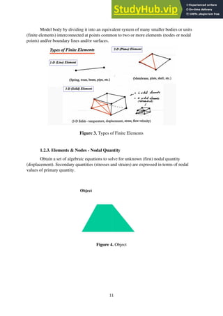
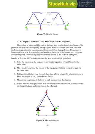
3.1.2.5. Apply The Boundary Conditions And Loads
The following boundary conditions apply to this problem: nodes A is pinned support
and C is roller support, which implies that 𝑈𝐴𝑥 = 0, 𝑈𝐴𝑦= 0, and 𝑈𝐶𝑦= 0. Incorporating these
conditions into the global stiffness matrix and applying the external loads at nodes E and D
such that 𝐹𝐸𝑦 = -2000 N and 𝐹𝐷𝑦 = -1000 N results in a set of linear equations that must be
solved simultaneously:
108
[
1 0 0 0 0 0 0 0 0 0
0 1 0 0 0 0 0 0 0 0
0 0 5 0 −2 0 −0.5 0.86 −0.5 −0.86
0 0 0 3 0 0 0.86 −1.5 −0.86 −1.5
0 0 −2 0 2.5 0 0 0 −0.5 0.86
0 0 0 0 0 1 0 0 0 0
0 0 −0.5 0.86 0 0 3 0 −2 0
0 0 0.86 −1.5 0 0 0 3 0 0
0 0 −0.5 −0.86 −0.5 0 −2 0 3 0
0 0 −0.86 −1.5 0.86 0 0 0 0 3 ]
(
𝑈𝐴𝑥
𝑈𝐴𝑦
𝑈𝐵𝑥
𝑈𝐵𝑦
𝑈𝐶𝑥
𝑈𝐶𝑦
𝑈𝐸𝑥
𝑈𝐸𝑦
𝑈𝐷𝑥
𝑈𝐷𝑦)
=
(
0
0
0
0
0
0
0
−2000𝑁
0
−1000𝑁)
Because 𝑈𝐴𝑥 = 0, 𝑈𝐴𝑦= 0, and 𝑈𝐶𝑦= 0, we can eliminate the first, second, and sixth rows and
columns from our calculation such that we need only solve a 7 X 7matrix:
108
[
5 0 −2 −0.5 0.86 −0.5 −0.86
0 3 0 0.86 −1.5 −0.86 −1.5
−2 0 2.5 0 0 −0.5 0.86
−0.5 0.86 0 3 0 −2 0
0.86 −1.5 0 0 3 0 0
−0.5 −0.86 −0.5 −2 0 3 0
−0.86 −1.5 0.86 0 0 0 3 ] (
𝑈𝐵𝑥
𝑈𝐵𝑦
𝑈𝐶𝑥
𝑈𝐸𝑥
𝑈𝐸𝑦
𝑈𝐷𝑥
𝑈𝐷𝑦)
=
(
0
0
0
0
−2000𝑁
0
−1000𝑁)
3.1.3. Solution Phase
3.1.3.1. Solve A System Of Algebraic Equations Simultaneously
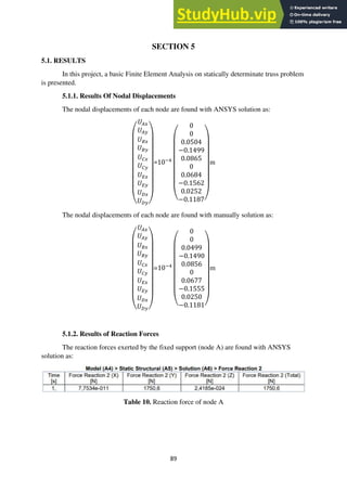
Solving the above matrix for the unknown displacements yields 𝑈𝐵𝑥=0.0499𝑋10−4
m,
𝑈𝐵𝑦=−0.1490𝑋10−4
m, 𝑈𝐶𝑥 =0.0856𝑋10−4
m, 𝑈𝐸𝑥 =0.0677𝑋10−4
𝑚,
𝑈𝐸𝑦=−0.1555𝑋10−4
m, and 𝑈𝐷𝑥 =0.0250𝑋10−4
𝑚, 𝑈𝐷𝑦 = −0.1181𝑋10−4
𝑚 Thus, the
global displacement matrix is
(
𝑈𝐴𝑥
𝑈𝐴𝑦
𝑈𝐵𝑥
𝑈𝐵𝑦
𝑈𝐶𝑥
𝑈𝐶𝑦
𝑈𝐸𝑥
𝑈𝐸𝑦
𝑈𝐷𝑥
𝑈𝐷𝑦)
=10−4
(
0
0
0.0499
−0.1490
0.0856
0
0.0677
−0.1555
0.0250
−0.1181)
m](https://image.slidesharecdn.com/analysisofatrussusingfiniteelementmethods-230804175539-9cf69e62/85/ANALYSIS-OF-A-TRUSS-USING-FINITE-ELEMENT-METHODS-85-320.jpg)
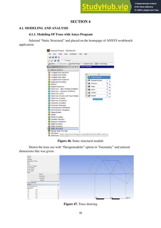
![75
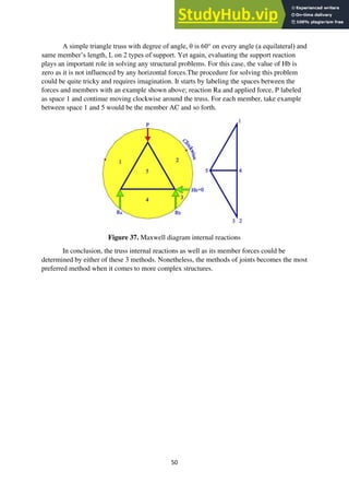
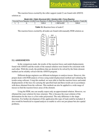
The reaction forces can be computed from,
{R}= [𝑲]𝐺
{U} – {F}
such that
(
𝑅𝐴𝑥
𝑅𝐴𝑦
𝑅𝐵𝑥
𝑅𝐵𝑦
𝑅𝐶𝑥
𝑅𝐶𝑦
𝑅𝐸𝑥
𝑅𝐸𝑦
𝑅𝐷𝑥
𝑅𝐷𝑦)
=108
[
2.5 0.86 −2 0 0 0 −0.5 −0.86 0 0
0.86 1.5 0 0 0 0 −0.86 −1.5 0 0
−2 0 5 0 −2 0 −0.5 0.86 −0.5 −0.86
0 0 0 3 0 0 0.86 −1.5 −0.86 −1.5
0 0 −2 0 2.5 −0.86 0 0 −0.5 0.86
0 0 0 0 −0.86 1.5 0 0 0.86 −1.5
−0.5 −0.86 −0.5 0.86 0 0 3 0 −2 0
−0.86 −1.5 0.86 −1.5 0 0 0 3 0 0
0 0 −0.5 −0.86 −0.5 0.86 −2 0 3 0
0 0 −0.86 −1.5 0.86 −1.5 0 0 0 3 ]
10−4
(
0
0
0.0499
−0.1490
0.0856
0
0.0677
−0.1555
0.0250
−0.1181)
-
(
0
0
0
0
0
0
0
−2000
0
−1000)
That the entire stiffness, displacement, and load matrices are used. Performing matrix
operations yields the reaction results
(
𝑅𝐴𝑥
𝑅𝐴𝑦
𝑅𝐵𝑥
𝑅𝐵𝑦
𝑅𝐶𝑥
𝑅𝐶𝑦
𝑅𝐸𝑥
𝑅𝐸𝑦
𝑅𝐷𝑥
𝑅𝐷𝑦)
=
(
0.8
1750.28
−2.14
1.22
1.34
1250.34
0.1
0.86
−0.1
−0.98 )
N](https://image.slidesharecdn.com/analysisofatrussusingfiniteelementmethods-230804175539-9cf69e62/85/ANALYSIS-OF-A-TRUSS-USING-FINITE-ELEMENT-METHODS-86-320.jpg)

![91
REFERENCES
[1] FINITE ELEMENT ANALYSIS: THEORY AND APPLICATION WITH ANSYS, 4th edition, ISBN
978-0-13-384080-3, by Saeed Moaveni, published by Pearson Education © 2015.
[2] THERMOMECHANICAL FINITE ELEMENT MODELING OF STEEL LADLE CONTAINING
ALUMINA SPINEL REFRACTORY LINING, Soheil Samadi, Shengli Jin, Dietmer Gruber, Harald
Harmuth, Finite Elements in Analysis and Design 206 (2022) 103762, Leoben, 8700, Austria.
[3] THE FINITE ELEMENT METHOD: THEORY, IMPLEMENTATION, AND APPLICATIONS, Larson
M. Springer, New York, 2013.
[4] FINITE ELEMENT METHODS, Schwab C., Oxford University Press, New York, 1998.
[5] ADVANCES IN FINITE ELEMENT METHOD, Song Cen, Chenfeng Li, Sellakkutti Rajendran,
and Zhiqiang Hu, 4 State Key Laboratory of Ocean Engineering, Shanghai Jiao Tong
University, Shanghai 200240, China, March 2014.
[6] FINITE ELEMENT METHOD: AN OVERVIEW, Vishal JAGOTA , Aman Preet Singh SETHI and
Khushmeet KUMAR, Department of Mechanical Engineering, Shoolini University, Solan,
India, January 2013.
[7] 3D FINITE ELEMENT ANALYSIS OF A CONCRETE DAM BEHAVIOR UNDER CHANGING
HYDROSTATIC LOAD A CASE STUDY, Pavel Žvanut, Slovenian National Building and Civil
Engineering Institute, Ljubljana, Slovenia
[8] FINITE ELEMENT ANALYSIS OF SPACE TRUSS USING MATLAB, P. Sangeetha, P. Naveen
Kumar and R.Senthil, India College of Engineering, Guindy, Anna University, Chennai, India,
ARPN Journal of Engineering and Applied Sciences, ISSN 1819-6608, VOL. 10, NO. 8, MAY
2015](https://image.slidesharecdn.com/analysisofatrussusingfiniteelementmethods-230804175539-9cf69e62/85/ANALYSIS-OF-A-TRUSS-USING-FINITE-ELEMENT-METHODS-102-320.jpg)
![92
[9] ANALYSIS OF A SELECTED NODE OF A TRUSS MADE OF COLDROLLED SECTIONS BASED ON
THE FINITE ELEMENT METHOD, Maciej MAJOR, Izabela MAJOR, Jaroslaw KALINOWSKI,
Mariusz KOSIN, DOI: 10.31490/tces-2018-0011, VOLUME: 18 | NUMBER: 2 | 2018 |
[10] COMPUTER-AIDED DESIGN METHODS FOR ADDITIVE FABRICATION OF TRUSS
STRUCTURES, Hongqing Wang, David Rosen, The George W. Woodruff School of Mechanical
Engineering Georgia Institute of Technology Atlanta, GA 30332-0405 USA 404- 894- 9668,
May 2014
[11] FINITE ELEMENT ANALYSIS ON CANTILEVER TRUSS USING NODAL DISPLACEMENT
METHOD, Yash Thakur, Yash Yogesh Bichu, Prathamesh Belgaonkar, Ved Gavade, Yogita
Potdar, 590008, India, International Research Journal of Engineering and Technology (IRJET)
e-ISSN: 2395-0056 Volume: 08 Issue: 06 | June 2021
[12] COMPUTING OF TRUSS STRUCTURE USING MATLAB, Alžbeta Bakošová, Jan Krmela,
Marián Handrik, Faculty of Industrial Technologies in Púchov, Alexander Dubček University
of Trenčín. Ivana Krasku 491/30, 02001 Púchov. August 2020, Vol. 20, No. 3
MANUFACTURING TECHNOLOGY ISSN 1213–2489, 279 DOI: 10.21062/mft.2020.059 © 2020
[13] TEACHING FINITE ELEMENT ANALYSIS AS A SOLUTION METHOD FOR TRUSS PROBLEMS
IN STATICS, Jiaxin Zhao Indiana University–Purdue University Fort Wayne, Session 1566,
American Society for Engineering Education Annual Conference & Exposition, American
Society for Engineering, 2004.
[14] ANALYSIS OF STATICALLY DETERMINATE TRUSSES, THEORY OF STRUCTURES, Asst. Prof.
Dr. Cenk Üstündağ.
[15] THE FINITE ELEMENT METHOD: ITS BASIS AND FUNDAMENTALS (6th ed.), Zienkiewicz,
O.C., Taylor R.L., Zhu J.Z., Oxford, UK: Elsevier Butterworth Heinemann, ISBN 978-07506632,
(2005).
[16] TRUSS OPTIMIZATION WITH DISCRETE DESIGN VARIABLES: A CRITICAL REVIEW, Mathias
Stolpe, Struct Multidisc Optim (2016) 53:349–374 DOI 10.1007/s00158-015-1333-x,
Springer-Verlag Berlin Heidelberg 2015.](https://image.slidesharecdn.com/analysisofatrussusingfiniteelementmethods-230804175539-9cf69e62/85/ANALYSIS-OF-A-TRUSS-USING-FINITE-ELEMENT-METHODS-103-320.jpg)
![93
[17] BENDING BEHAVIOR OF COMPOSITE SANDWICH STRUCTURES WITH GRADED
CORRUGATED TRUSS CORES, Yang Suna , Li-cheng Guoa, Tian-shu Wanga, Su-yang Zhonga,
Hai-zhu Pan, ScienceDirect Volume 185, Pages 446-454 February 2018.
[18] https://skyciv.com/docs/tutorials/truss-tutorials/types-of-truss-structures/ , December
8, 2021
[19] SHAPE AND CROSS-SECTION OPTIMISATION OF A TRUSS STRUCTURE. IN: COMPUTERS
AND STRUCTURES. GIL, L., ANDREU, Vol. 79, pp. 681 – 689, (2000).](https://image.slidesharecdn.com/analysisofatrussusingfiniteelementmethods-230804175539-9cf69e62/85/ANALYSIS-OF-A-TRUSS-USING-FINITE-ELEMENT-METHODS-104-320.jpg)

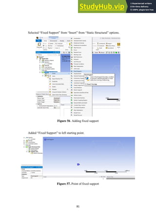
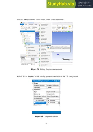
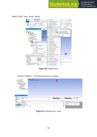
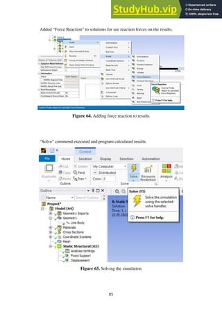
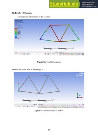
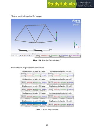
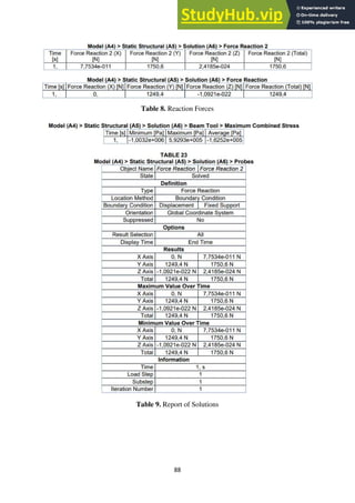
This document describes a project analyzing a truss structure using finite element methods. It begins with an introduction to finite element analysis and its history. It then provides the fundamentals of finite element analysis and matrix algebra used in the method. Next, it discusses truss structures and various methods for truss analysis. The document then gives an example of determining the reaction forces of a truss manually using finite element formulations. Finally, it models the same example truss in ANSYS and compares the results of the manual and ANSYS solutions.