This document summarizes Luigi Gigliotti's 2012 master's thesis which assessed the applicability of the extended finite element method (XFEM) in Abaqus software for modeling crack growth in rubber materials. The thesis first reviewed rubber elasticity, fracture mechanics of rubber, and XFEM. It then formulated static and dynamic analysis problems to evaluate XFEM's ability to model stress/displacement fields and predict crack propagation instant, direction, and speed using neo-Hookean and Arruda-Boyce material models. Results showed XFEM accurately modeled displacement fields but provided no benefits over FEM for stress fields. Difficulties were faced achieving convergence for dynamic analyses. The thesis aimed to help

![Chapter 1
Fundamentals: literature review and
basic concepts
1.1 Rubber elasticity
Rubber-like materials, such as rubber itself, soft tissues etc, can be appropriately described by virtue of a well-know
theory in the continuum mechanics framework, named Hyperelasticity Theory. For this purpose, in this section the
fundamental aspects of this theory - albeit limited to the case of isotropic and incompressible material - as well as
finite displacements and deformations theory will be expounded [1]. Lastly, a description of the hyperelastic constitutive
models adopted in this work is proposed.
1.1.1 Kinematics of large displacements
The main goal of the kinematics theory, is to study and describe the motion of a deformable body, i.e to determine its
successive configurations under a general defined load condition, as function of the pseudo-time t.
A deformable body, within the framework of 3D Euclidean space, R3
, can be regarded as a set of interacting particles
embedded in the domain Ω ∈ R3
(see Fig. 1.1). The boundary of this latter, often referred to as Γ = ∂Ω is split up in two
different parts, Γu along which the displacement values are prescribed and Γσ where the stress component values have to
be imposed. A problem is said to be well-posed if these two different boundary conditions are not applied simultaneously
on the same portion of frontier. Moreover, the boundary Γ should be characterized by a sufficient smoothness (at least
piece-wise), in order to define uniquely the outward unit normal vector n; last but not least, it must be highlighted that,
a unique solution of the boundary value problem is achievable only if Γu = ∅, such that all the rigid body motions are
eliminated.
Figure 1.1: Initial and deformed configurations of a solid deformable body in 3D Euclidean space.
Among all possible configurations assumed by a deformable body during its motion, of particular importance is the
reference (or undeformed) configuration Ω, defined at a fixed reference time and depicted in Fig. 1.1 with the
dashed line. With excess of meticulousness, it is worth noting that a so-called initial configuration at initial time t = 0,
can be defined and that, whilst for static problems such configuration coincides with the reference one, in dynamics the
initial configuration is often not chosen as the reference configuration. In the reference configuration, every particles of
1](https://image.slidesharecdn.com/5bffcdff-873e-4f02-b330-da222b639ff8-151115100138-lva1-app6891/75/FULLTEXT01-7-2048.jpg)
![1.1. RUBBER ELASTICITY L. Gigliotti 3
The tangent vectors dx and dxϕ
are usually labelled as material (or undeformed) line element and spatial (or
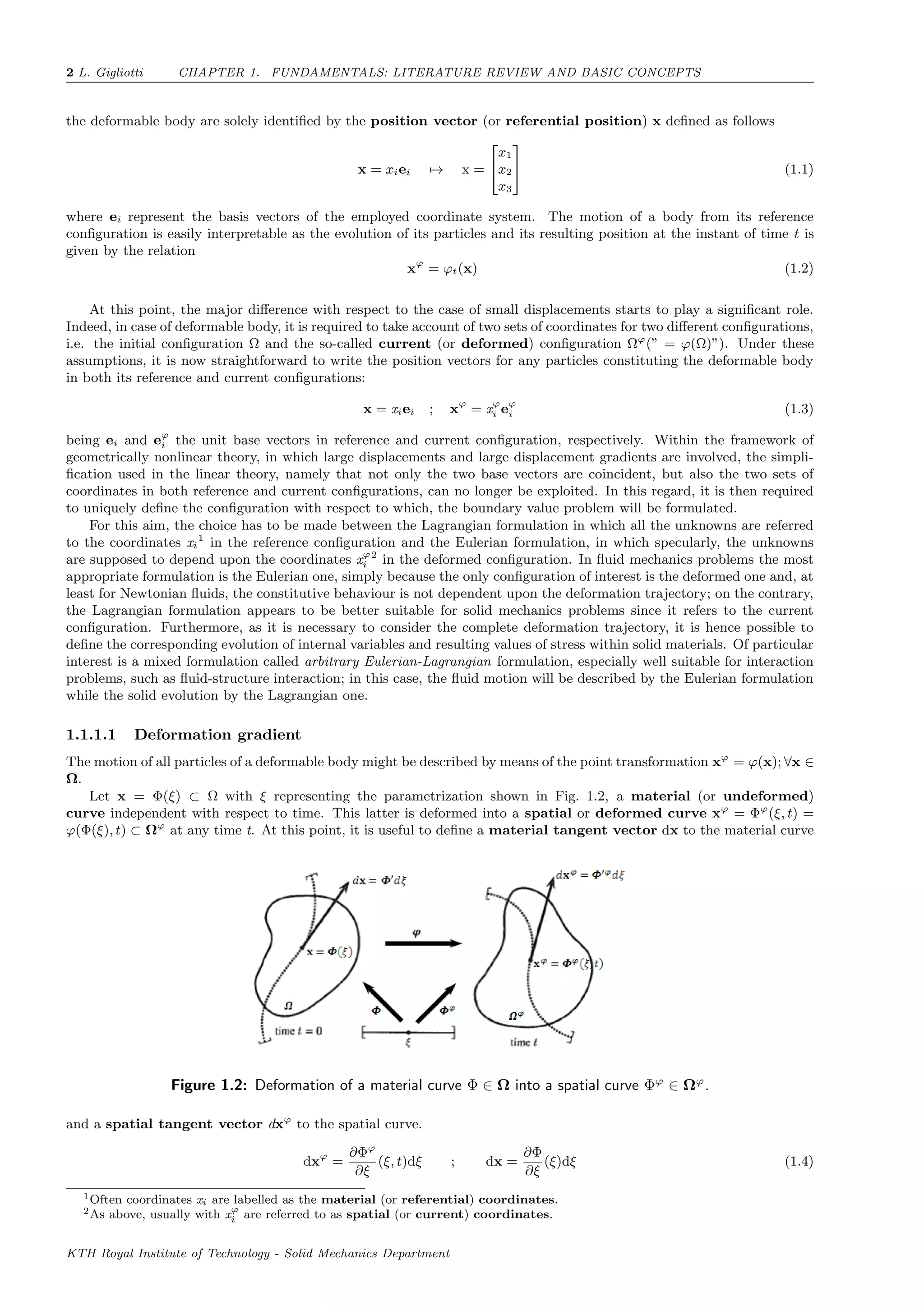
deformed) line element, respectively. Furthermore, for any motion taking place in the Euclidean space, a large
displacement vector can be introduced as follows
d(x) = xϕ
⇔ di(x) = ϕjδij − xi (1.5)
According to Fig. 1.3, and by means of basic notions of algebra of tensors, it is possible to infer that:
Figure 1.3: Total displacement field.
xϕ
+ dxϕ
= x + dx + d(x + dx) =⇒ dxϕ
= dx + d(x + dx) − d(x) (1.6)
The term d(x + dx) can be computed by exploiting Taylor series formula, and truncating them after the linear term:
d(x + dx) = d(x) + d(x)dx + o( dx ) (1.7)
where, d is the large displacement gradient, or in index notation
di(x + dx) = di(x) +
∂di
∂xi
(x)dxi + o( dx ) (1.8)
At this point, it is sufficient to compare Eq. 1.6 and Eq. 1.7, to express the spatial tangent vector dxϕ
as function of its
corresponding material tangent vector and of the two-point tensor F named as deformation gradient tensor:
dxϕ
= (I + d)
F
dx ⇒ dxϕ
= Fdx ; [F]ij :=
∂xi
∂xj
+
∂di
∂xj
=
∂ϕi
∂xj
(1.9)
or alternatively,
F =
∂ϕi
∂xj
eϕ
i ⊗ ej ; F = ϕ ⊗ (1.10)
with the gradient operator = ∂
∂xj
ei.
It is a painless task to demonstrate how the deformation gradient, not only provides the mapping of a generic
(infinitesimal) material tangent vector into the relative spatial tangent vector, but also controls the transformation of an
infinitesimal surface element or an infinitesimal volume element (see Fig. 1.4).
Figure 1.4: Transformation of infinitesimal surface and volume elements between initial and deformed
configuration.
KTH Royal Institute of Technology - Solid Mechanics Department](https://image.slidesharecdn.com/5bffcdff-873e-4f02-b330-da222b639ff8-151115100138-lva1-app6891/75/FULLTEXT01-9-2048.jpg)
![4 L. Gigliotti CHAPTER 1. FUNDAMENTALS: LITERATURE REVIEW AND BASIC CONCEPTS
Let dA be an infinitesimal surface element, constructed as the vector product of two infinitesimal reciprocally orthog-
onal vectors, dx and dy; the outward normal vector is, as usual, defined as n = (dx × dy)/ dx × dy . By means of the
deformation gradient F, the new extension and orientation in the space of the surface element can be easily determined
dAϕ
nϕ
:= dxϕ
× dyϕ
= (Fdx) × (Fdy) = (det [F] F−T
)(dx × dy)
dAn
= dA(cof [F])n (1.11)
which is often referred to as Nanson’s formula.
Once the Nanson’s formula has been derived, it is straightforward to obtain the analogous relation for the change of an
infinitesimal volume element occurring between the initial and the deformed configuration. Describing the infinitesimal
volume element in the material configuration as the scalar product between an infinitesimal surface element dAϕ
and
the infinitesimal vector dzϕ
and exploiting results in Eq. 1.11, the following relation holds
dV ϕ
:= dzϕ
· dAnϕ
= Fdz · JF−T
dAn = Jdz · dAn = JdA (1.12)
in which J = det [F] is well-known as the Jacobian determinant (or volume ratio).
As stated in Eq. 1.9, the deformation gradient F, is a linear transformation of an infinitesimal material vector dx into
its relative spatial dxϕ
; such transformation affects all parameters characterizing a vector, its modulus, direction and
orientation. However, the deformation is related only to the change in length of an infinitesimal vector, and therefore,
it results to be handy to consider the so-called polar decomposition, by virtue of which the deformation gradient can
be written as a multiplicative split between an orthogonal tensor R, an isometric transformation which only changes the
direction and orientation of a vector, and a symmetric, positive-definite stretch tensor U that provides the measure of
large deformation.
F = RU ; RT
= R−1
; UT
= U ; dxϕ
= Ux (1.13)
In other words, the symmetric tensor U, yet referred in literature to as the right (or material) stretch tensor,
produces a deformed vector that remains in the initial configuration (no large rotations). In index notation, the large
rotations tensor R, and the right stretch tensor U, can be respectively expressed as follows
R = Rijeϕ
i ⊗ ej ; U = Uijei ⊗ ej (1.14)
An alternative form of the polar decomposition can be provided, by simply inverting the order of the above mentioned
transformations and introducing the so-called left(or spatial) stretch tensor V
F = VR ; V = Vijeϕ
i ⊗ eϕ
j (1.15)
In such case, a large rotation, represented by R, is followed by a large deformation (tensor V).
1.1.1.2 Strain measures
Theoretically, apart form the right and the left stretch tensors U and V, an infinite number of other deformation measures
can be defined; indeed, unlike displacements, which are measurable quantities, strains are based on a concept that is
introduced as a simplification for the large deformation analysis.
From a computational point of view, the choice or U or V to calculate the stress values is not the most appropriate
one, as it requires, first, to perform the polar decomposition of the deformation gradient. Hence, it is necessary to
introduce deformation measures that can directly, without any further computations, provide information about the
deformation state.
We may consider two neighbouring points defined by their position vectors x and y in the material description; with
reference to Fig. 1.5 on the next page, it is possible to describe the relation between these two, sufficiently close points,
i.e.
y = y + (x − x) = x + y − x
y − x
y − x
= x + dx (1.16)
dx = dεa and dε = y − x , a =
y − x
y − x
(1.17)
In the above equations, it is clear that the length of the material line element dx is denoted by the scalar value dε
and that the unit vector a, with a = 1, represents the direction of the aforesaid vector at the given position in the
reference configuration. As stated in Eq. 1.9, the deformation gradient F allows to linearly approximate a vector dx in
the material description, with its corresponding vector dxϕ
in the spatial description. The smaller the vector dx, the
better the approximation.
At this point, it is then possible to define the stretch vector λa, in the direction of the unit vector a and at the point
x ∈ Ω as
λa(x, t) = F(x, t)a (1.18)
with its modulus λ known as stretch ratio or just stretch. This latter is a measure of how much the unit vector a has
been stretched. In relation to its value, λ < 1, λ = 1 or λ > 1, the line element is said to be compressed, unstretched
KTH Royal Institute of Technology - Solid Mechanics Department](https://image.slidesharecdn.com/5bffcdff-873e-4f02-b330-da222b639ff8-151115100138-lva1-app6891/75/FULLTEXT01-10-2048.jpg)
![1.1. RUBBER ELASTICITY L. Gigliotti 5
Figure 1.5: Deformation of a material line element with length dε into a spatial element with length
λdε.
or extended, respectively. Computing the square of the stretch ratio λ, the definition of the right Cauchy-Green
tensor C is introduced
λ2
= λa · λa = Fa · Fa = a · FT
Fa = a · Ca ,
C = FT
F or CIJ = FiI FiJ
(1.19)
Often the tensor C is also referred to as the Green deformation tensor and it should be highlighted that, since the
tensor C operate solely on material vectors, it is denoted as a material deformation tensor. Moreover, C is symmetric
and positive definite ∀x ∈ Ω:
C = FT
F = (FT
F)T
= CT
and u · Cu > 0 ∀u = 0 (1.20)
The inverse of the right Cauchy-Green tensor is the well-known Piola deformation tensor B, i.e. B = C−1
.
To conclude the roundup of material deformation tensors, the definition of the commonly used Green-Lagrange
strain tensor E, is here provided:
1
2
(λdε)2
− dε2
= 1
2
(dεa) · FT
F (dεa) − dε2
= dx · Edx ,
E = 1
2
FT
F − I = 1
2
(C − I) or EIJ = 1
2
(FiI FiJ − δIJ )
(1.21)
whose symmetrical nature is obvious, given the symmetry of C and I. In an analogous manner of the one shown above,
it is possible to describe deformation measures in spatial configuration, too; the stretch vector λaϕ in the direction of
aϕ
, for each xϕ
∈ Ω might thus be define as:
λ−1
aϕ (xϕ
, t) = F−1
(xϕ
, t)aϕ
(1.22)
where, the norm of the inverse stretch vector λ−1
aϕ is called inverse stretch ratio λ−1
or simply inverse stretch.
Moreover, the unit vector aϕ
may be interpreted as a spatial vector, characterizing the direction of a spatial line element
dxϕ
. By virtue of Eq. 1.22, computing the square of the inverse stretch ratio, i.e.
λ−2
= λ−1
aϕ · λ−1
aϕ = F−1
a · F−1
a = a · F−T
F−1
a = a · b−1
a (1.23)
where b is the left Cauchy-Green tensor, sometimes referred to as the Finger deformation tensor
b = FFT
or bij = FiI FjI (1.24)
Like its corresponding tensor in the material configuration, the Green deformation tensor, the left Cauchy-Green tensor
b is symmetric and positive definite ∀xϕ
∈ Ω:
b = FFT
= (FT
F)T
= bT
and u · bu > 0 ∀u = 0 (1.25)
Last but not least, the well-known symmetric Euler-Almansi strain tensor e is here introduced:
1
2
[d˜ε2
− (λ−1
d˜ε)2
] =
1
2
[d˜ε2
− (d˜εa) · F−T
F−1
(d˜εa)] = dxϕ
· edxϕ
,
e =
1
2
(I − F−T
F−1
) or eij =
1
2
(δij − F−1
Ki F−1
Kj )
(1.26)
where the scalar value d˜ε is the (spatial) length of a spatial line element dxϕ
= xϕ
− yϕ
.
KTH Royal Institute of Technology - Solid Mechanics Department](https://image.slidesharecdn.com/5bffcdff-873e-4f02-b330-da222b639ff8-151115100138-lva1-app6891/75/FULLTEXT01-11-2048.jpg)
![1.1. RUBBER ELASTICITY L. Gigliotti 7
In addition, the so-called second Piola-Kirchhoff stress tensor S has been proposed, especially for its noticeable
usefulness in the computational mechanics field, as well as for the formulation of constitutive equations; this contravariant
material tensor does not have any physical interpretation in terms of surface tractions and it can be easily computed by
applying the pull-back operation on the contravariant spatial tensor τ:
S = F−1
τF−T
or SIJ = F−1
Ii F−1
Jj τij (1.32)
The second Piola-Kirchhoff stress tensor S can be, moreover, related to the Cauchy stress tensor by exploiting Eqs.
1.29, 1.32 and 1.31:
S = JF−1
σF−T
= F−1
P = ST
or SIJ = JF−1
Ii F−1
Jj σij = F−1
Ii PiJ = SJI (1.33)
as consequence, the fundamental relationship between the first Piola-Kirchhoff stress tensor P and the symmetric second
Piola-Kirchhoff stress tensor S is found, i.e.
P = FS or PiI = FiJ SJI (1.34)
A plethora of other stress tensors can be found in literature; among them the Biot stress tensor TB, the symmetryc
corotated Cauchy stress tensor σu and the Mandel stress tensor Σ deserve to be mentioned [2].
1.1.2 Hyperelastic materials
The correct formulation of constitutive theories for different kinds of material, is a very important matter in continuum
mechanics, in particular with regards to the description of nonlinear materials, such as rubber-like ones.
The branch of continuum mechanics, which provides the formulation of constitutive equations for that category of ma-
terials which can sustain to large deformations, is called finite (hyper)elasticity theory or just finite (hyper)elasticity.
In this theory, the existence of the so-called Helmoltz free-energy function Ψ, defined per unit reference volume or
alternately per unit mass, is postulated. In the most general case, the Helmoltz free-energy function is a scalar-
valued function of the tensor F and of the position of the particular point within the body. Restricting the analysis
to the case of homogeneous material, the energy solely depends on the deformation gradient F, and as such, it is often
referred to as strain-energy function or stored-energy function Ψ = Ψ(F). By virtue of what has been shown in
the previous section, the strain energy function Ψ can be expressed as function of several other deformation tensors, e.g.
the right Cauchy-Green tensor C, the left Cauchy-Green tensor b.
A hyperelastic material, or Green-elastic material, is a subclass of elastic materials for which the relation expressed
in Eq. 1.35 holds
P = G(F) =
∂Ψ(F)
∂F
or PiI =
∂Ψ
∂FiI
(1.35)
Many other reduced forms of constitutive equations, equivalent to the latter, for hyperelastic materials at finite strains
can be derived; while not wishing to report here all the different forms available in literature, consider for this purpose,
the derivative with respect to time of the strain energy function Ψ(F):
˙Ψ = tr
∂Ψ(F)
∂F
T
˙F = tr
∂Ψ(C)
∂C
˙C =
= tr
∂Ψ(C)
∂C
˙FT
F + FT ˙F = 2tr
∂Ψ(C)
∂C
FT ˙F
(1.36)
Given the symmetry of the tensor C, and the resulting symmetry of the tensor valued scalar function Ψ(C), it follows
immediately that:
∂Ψ(F)
∂F
T
= 2
∂Ψ(C)
∂C
FT
(1.37)
1.1.2.1 Isotropic hyperelastic materials
Within the context of hyperelasticity, a typology of materials of unquestionable importance, of which rubber is one of
the most representative examples, consists of the so-called isotropic materials. From a physical point of view, the
property of isotropy is nothing more than the independence in the response of the material, in terms of stress-strain
relations, with respect to the particular direction considered.
Let us consider a point within an elastic, deformable body occupying the region Ω and identified by its position
vector x. Furthermore, let the body, in the reference configuration, undergo a translational motion represented by the
vector c and rotated through the orthogonal tensor Q (see Fig. 1.7 on the following page):
x∗
= c + Qx (1.38)
The deformation gradient F that links the material configuration Ω∗
, to the spatial configuration Ωϕ∗
might be computed
KTH Royal Institute of Technology - Solid Mechanics Department](https://image.slidesharecdn.com/5bffcdff-873e-4f02-b330-da222b639ff8-151115100138-lva1-app6891/75/FULLTEXT01-13-2048.jpg)
![8 L. Gigliotti CHAPTER 1. FUNDAMENTALS: LITERATURE REVIEW AND BASIC CONCEPTS
Figure 1.7: Rigid-body motion superimposed on the reference configuration.
by making use of the chain rule and Eq. 1.38, leading to
F =
∂xϕ
∂x
=
∂xϕ
∂x∗
Q = F∗
Q or FiI =
∂xϕ
i
∂xI
=
∂xϕ
i
∂x∗
J
QJI = F∗
iJ QJI (1.39)
A material is said to be isotropic if, and only if, the strain energies defined with respect to the deformation gradients F
and F∗
are the same for all orthogonal vectors Q; thus, it might be written that:
Ψ(F) = Ψ(F∗
) = Ψ(FQT
) (1.40)
which is the unavoidable condition to refer to a material as isotropic.
Ψ(C) = Ψ(F∗T
F∗
) = Ψ(QFT
FQT
) = Ψ(C∗
) (1.41)
Hence, if this latter relation is valid for all symmetric tensors C and all orthogonal tensors Q, the strain energy function
Ψ(C), is a scalar-valued isotropic tensor function solely of the tensor C. Under these assumption, the strain energy
might be expressed in terms of its invariants, i.e. Ψ = Ψ [I1 (C) , I2 (C) I3 (C)] or, equivalently, of its principal stretches
Ψ = Ψ (C) = Ψ [λ1, λ2, λ3].
1.1.2.2 Incompressible hyperelastic materials
A category of rubber-like materials widely used in practical applications and therefore particularly attractive, especially
with regard to the corresponding computational analysis by means of numerical codes, are the so-called incompressible
materials, which can sustain finite strains without show any considerable volume changes. In reference to Eq. 1.12, it
might to be stated that, the incompressibility constraint can be expressed as:
J = 1 (1.42)
The incompressibility constraint is widely known in literature as an internal constraint and a material subjected to
such constraint is called constrained material. In order to derive constitutive equations for a general incompressible
material, it is necessary to postulate the existence of a particular strain energy function:
Ψ = Ψ(F) − p(J − 1) (1.43)
defined exclusively for J = det(F) = 1. In such expression, the scalar parameter p, is referred to as Lagrange multiplier,
whose value can be determined by solving the equations of equilibrium. As proven in the previous sections, it is sufficient,
assuming that this is possible, to differentiate the strain energy function in Eq. 1.43 with respect to the deformation
gradient F, to obtain the three fundamental constitutive equations in terms of the first and the second Piola-Kirchhoff
stresses, i.e. P and S, and of the Cauchy stress tensor σ. For the particular case of incompressible materials, they may
be written as
P = −pP−T
+
∂Ψ(F)
∂F
S = −pF−1
F−T
+ F−1 ∂Ψ(F)
∂F
= −pC−1
+ 2
∂Ψ(C)
∂C
σ = −pI +
∂Ψ(F)
∂F
FT
= −pI + F
∂Ψ(F)
∂F
T
(1.44)
KTH Royal Institute of Technology - Solid Mechanics Department](https://image.slidesharecdn.com/5bffcdff-873e-4f02-b330-da222b639ff8-151115100138-lva1-app6891/75/FULLTEXT01-14-2048.jpg)
![1.1. RUBBER ELASTICITY L. Gigliotti 9
Additionally, it has been demonstrated formerly that, in the case of isotropic material, the strain energy function can
be expressed as function of the right Cauchy Green tensor C, the left Cauchy-Green tensor b and their invariants.
However, if the material is at the same time incompressible and isotropic, it is also true that I3 = det C = det b = 1
and consequently, the third invariant is no longer an independent deformation variable like I1 and I2. Consequently, the
relation stated in 1.43 can be reformulated as follows
Ψ = Ψ [I1(C), I2(C)] −
1
2
p(I3 − 1) = Ψ [I1(b), I2(b)] −
1
2
p(I3 − 1) (1.45)
Thus, the associated constitutive equations are written as
S = 2
∂Ψ(I1, (I1)
∂C
−
∂[p(I3 − 1)]
∂C
= −pC−1
+ 2
∂Ψ
∂I1
+ I1
∂Ψ
∂I2
I − 2
∂Ψ
∂I2
C
σ = −pI + 2
∂Ψ
∂I1
+ I1
∂Ψ
∂I2
b − 2
∂Ψ
∂I2
b2
= −pI + 2
∂Ψ
∂I1
b − 2
∂Ψ
∂I2
b−1
(1.46)
Lastly, if the strain energy function is expressed as a function of the three principal stretches λi, it holds that
Si = −
1
λ2
i
p +
1
λi
∂Ψ
∂λi
, i = 1, 2, 3 (1.47)
Pi = −
1
λi
p +
∂Ψ
∂λi
, i = 1, 2, 3 (1.48)
σi = −p + λi
∂Ψ
∂λi
, i = 1, 2, 3 (1.49)
for whom the constraint of incompressibility, i.e. J = 1 takes the following form:
λ1λ3λ3 = 1 (1.50)
1.1.3 Isotropic Hyperelastic material models
Due to the greater difficulty in the mathematical treatment of hyperelastic materials, there are several examples in
literature about possible forms of strain energy functions for compressible, as well as for incompressible materials.
In the following sections, the two models adopted in the present work, i.e. the Arruda-Boyce and the Neo-
Hookean model, will be described. It must be stressed however that, exclusively isotropic incompressible material
models under isothermal regime have been treated. Many other models have been proposed in literature, e.g. Ogden
model [4, 5] , Mooney-Rivlin model, [11], Yeoh model [16], Kilian-Van der Waals model [20] among the most
famous.
1.1.3.1 Neo-Hookean model
The Neo-Hookean model [6] can be referred to as a particular case of the Ogden model. Its mathematical expression is
the following one
Ψ = c1 λ2
1 + λ2
2 + λ2
3 − 3 = c1 (I1 − 3) (1.51)
By virtue of the consistency condition [7], it follows that
Ψ =
µ
2
λ2
1 + λ2
2 + λ2
3 − 3 (1.52)
where µ indicates the shear modulus in the reference configuration.
The neo-Hookean model, firstly proposed by Ronald Rivlin in 1948, is similar to the Hooke’s law adopted for linear
materials; indeed, the stress-strain relationship is initially linear while at a certain point the curve will level out. The
principal drawback of such model is its inability to predict accurately the behaviour of rubber-like materials for strains
larger then 20% and for biaxal stress states.
It can now be proven that, even if from a mathematical point of view, the Neo-Hookean model may be seen as the
simplest case of the Ogden model, it might be also justified within the context of the Gaussian statistical theory[8, 9]
of elasticity, which is based on the assumption that only small strains will be involved in the course of the deformation4
.
Briefly, rubber-like materials are made up of long-chain molecules, producing one giant molecule, referred to as molecular
4This fact is a further validation of the adequacy of neo-Hookean model for strains up to 20%; the more refined non-Gaussian
statistical theory, of which an example is based on the Langevin distribution function is needed, in order to obtain a more
accurate model for large strains.
KTH Royal Institute of Technology - Solid Mechanics Department](https://image.slidesharecdn.com/5bffcdff-873e-4f02-b330-da222b639ff8-151115100138-lva1-app6891/75/FULLTEXT01-15-2048.jpg)
![10 L. Gigliotti CHAPTER 1. FUNDAMENTALS: LITERATURE REVIEW AND BASIC CONCEPTS
network [10]; starting from the Boltzmann principle, and under the assumptions of incompressible material and affine
motion, the entropy change of this network, generated by the motion, can be readily computed as function of the number
N of chains in a unit volume of the network itself and of the principal stretches λi, i = 1, 2, 3
∆η = −
1
2
Nκ
r2
0in
r2
out
λ2
1 + λ2
2 + λ2
3 − 3 (1.53)
where κ = 1.38 · 10−23
Nm/K is the well-known Boltzmann’s constant; at the same time, the parameter r2
out and
r2
0in are the mean square value of the end-to-end distance of detached chains and of the end-to-end distance of cross-
linked chains in the network, respectively. For isothermal processes ˙Θ = 0 , the Legendre transformation leads to
the following expression for the Helmholtz free-energy function
Ψ =
1
2
NκΘ
r2
0in
r2
out
λ2
1 + λ2
2 + λ2
3 − 3 (1.54)
In conclusion, if the shear modulus µ is expressed as proportional to the concentration of chains N, it holds that:
µ = NκΘ
r2
0in
r2
out
(1.55)
By virtue of this latter result, the equivalence between Eqs. 1.51 and 1.54 is demonstrated.
1.1.3.2 Arruda-Boyce model
The second material model adopted in this work for modeling the response of rubber-like materials is the Arruda-Boyce
model [14], proposed in 1993; in this model, also known as the eight-chain model, the assumption that the molecular
network structure can be regarded as a representing cubic unit volume in which, eight chains are distributed along the
diagonal directions towards its eight corners, is made. The Arruda-Boyce model is particularly suitable to characterize
properties of carbon-black filled rubber vulcanizates; such a notable category of elastomers are reinforced with fillers like
carbon black or silica obtaining thus, a significant improvement in terms of tensile and tear strength, as well as abrasion
resistance. By virtue of these reasons, the stress-strain relation is tremendously nonlinear (stiffening effect) at the large
strains.
Unlike the neo-Hookean model, the Arruda-Boyce model is based on the non-Gaussian statistical theory [15]
and consequently is adequate to approximate the finite extensibility of rubber-like materials as well as the upturn effect
at higher strain levels. The strain energy function for the model considered herein, may be presented as
Ψ = NκΘ
√
n βλchain −
√
n ln
sinh β
β
(1.56)
The coefficients in the above written equation, are easily defined as follows
λchain = I1/3 and β = L−1 λchain
√
n
(1.57)
where, L is known as Langevin function; obviously, for computational reasons the latter function is approximated
with a Taylor series expansion. By making use of the first five terms of the Taylor expansion of the Langevin function,
a different analytical expression is given by
Ψ = c1
1
2
(I1 − 3)
1
20λ2
m
I2
1 − 9 +
11
1050λ4
m
I3
1 − 27 +
19
7000λ6
m
I4
1 − 81 +
519
673750λ8
m
I5
1 − 243 (1.58)
where λm is referred to as locking stretch, representing the stretch value at which the slope of the stress-strain curve
will rise significantly and thus, where the polymer chain network becomes locked. The consistency condition allows to
define the constant c1 as
c1 =
µ
1 + 3
5λ2
m
+ 99
175λ4
m
+ 513
875λ6
m
+ 42039
67375λ8
m
(1.59)
Lastly, it ought to be stressed that the strain energy function in the Arruda-Boyce model depends only upon the
first invariant I1; from a physical point of view, this means that the eight chains stretch uniformly along all directions
when subjected to a general deformation state.
A comparison of the quality of approximation for different material models is depicted in Fig. 1.8 on the next page;
according to this plot, it is inferable that not all material models show the same level of accuracy in predicting the
stress-strain behavior of rubber-like materials. In particular, some models, i.e. Neo-Hookean model and Mooney-Rivlin
model, exhibit the incapacity to model the stiffening effect at the high strains.
KTH Royal Institute of Technology - Solid Mechanics Department](https://image.slidesharecdn.com/5bffcdff-873e-4f02-b330-da222b639ff8-151115100138-lva1-app6891/75/FULLTEXT01-16-2048.jpg)
![1.2. FRACTURE MECHANICS OF RUBBER L. Gigliotti 11
Figure 1.8: Stress-strain curves for uniaxial extension conditions - Comparison among various hypere-
lastic material models.
1.2 Fracture Mechanics of Rubber
The extension of fracture mechanics concepts to elastomers has always represented a problem of major interest, since
the first work in this field has been presented by Rivlin and Thomas in 1952 [21]. In this cornerstone work the authors
have shown how large deformations of rubber render the solution of the boundary value problem of a cracked body
made of rubber, a quite compounded task. By virtue of the aforementioned nonlinear nature of constitutive models
and due to the capacity of rubber-like materials to undergo finite deformations, LEFM results cannot be, without prior
modifications, extended to this category of materials and thus, a slightly different approach has to be adopted. In this
section, some of the most relevant results achieved in the fracture mechanics of elastomers field, along with experimental
results, are briefly described and discussed.
1.2.1 Fracture mechanics approach
The introduction of fracture mechanics concepts goes back to Griffith’s experimental work on the strength of glass [22].
Griffith noticed that the characteristic tensile strength of the material was highly affected by the dimensions of the
component; by virtue of these observations, he pointed out that the variability of tensile strength should be related to
something different than a simple inherent material property. Previously, Inglis had demonstrated that the common
design procedure based on the theoretical strength of solid, was no longer adapt and that this material property should
have been reduced, in order to take into account the presence of flaws within the component5
.
Griffith [22] hypothesized that, in an analogous manner of liquids, solid surfaces are characterized by surface tension.
Having this borne in mind, for the propagation of a crack, or in order to increase its surface area, it is necessary that
the surface tension, related to the new propagated surface, is less than the energy furnished from the external loads, or
internally released. Alternatively, the Griffith-Irwin-Orowan theory [24] [25] [26] claims that a crack will run through a
solid deformable body, as soon as the input energy-rate surmounts the dissipated plastic-energy; denoting with W the
work done by the external forces, with Ue
s and Up
s the elastic and the plastic part of the total strain energy, respectively,
and with UΓ the surface tension energy, we may write thus
∂W
∂a
=
∂Ue
s
∂a
+
∂Up
s
∂a
+
∂UΓ
∂a
(1.60)
This expression might then be rewritten in terms of the potential energy Π = Ue
s − W, i.e.
−
∂Π
∂a
=
∂Up
s
∂a
+
∂UΓ
∂a
(1.61)
5In other words, the comparison ought to be made between the theoretical tensile strength and the concentrated stress and not
with the average stress computed by using the usual solid mechanics theory, based on the assumption of the absence of internal
defects.
KTH Royal Institute of Technology - Solid Mechanics Department](https://image.slidesharecdn.com/5bffcdff-873e-4f02-b330-da222b639ff8-151115100138-lva1-app6891/75/FULLTEXT01-17-2048.jpg)
![12 L. Gigliotti CHAPTER 1. FUNDAMENTALS: LITERATURE REVIEW AND BASIC CONCEPTS
which represents a stability criterion stating that, the decreasing rate of potential energy during crack growth must
equal the rate of dissipated energy in plastic deformation and crack propagation. Furthermore, Irwin demonstrated
that the input energy rate for an infinitesimal crack propagation, is independent of the load application modalities, e.g.
fixed-grip condition or fixed-force condition, and it is referred to as strain-energy release rate G, for a unit length increase
in the crack extension.
For the particular case of brittle materials, the plastic term Up
s vanishes and the following expression might be
deduced:
G = −
∂Π
∂a
= 2γs (1.62)
where γs is the surface energy and the term 2 is easily justified given the presence of two crack surfaces.
In one of his successive works, Griffith computed, in the case of an infinite plate with a central crack of length 2a
subjected to uniaxial tensile load (see Fig. 1.9), the strain energy needed to propagate the crack, showing that it is equal
to the energy needed to close the crack under the action of the acting stress
Figure 1.9: Infinite plate with central crack of length 2a, subjected to an uniaxial stress state.
Π = 4
a
0
σuy (x) dx =
πσ2
a2
2E
⇒ G = −
∂Π
∂a
=
πaσ2
E
(1.63)
where the coefficient E is defined below
E =
E Plane stress
E
1−ν2 Plane strain
(1.64)
being E the Young’s modulus.
Combining Eqs. 1.62 and 1.63 it is straightforward to obtain the critical stress for cracking as
σcr =
2E γs
πa
(1.65)
and the critical stress intensity factor KC
6
is given by
KC = σcr
√
πa (1.66)
The crack growth stability may be assessed by simply considering the second derivative of (Π + UΓ); namely, the
crack propagation will be unstable or stable, when the energy at equilibrium assumes its maximum or minimum value,
respectively [27]
∂2
(Π + UΓ)
∂a2
=
< 0 unstable fracture
= 0 stable fracture
> 0 neutral equilibrium
(1.67)
With certain modifications, in order to consider their different behaviour, e.g. the plastic deformation area in the
vicinity of the crack tip, Griffith theory has been extended to fracture processes of metallic materials. Hence, LEFM
became a powerful tool for post-mortem analysis to predict metals fracture, to characterize fatigue crack extension rate,
along with the identification of the threshold or lower bound below which fatigue and stable crack growth will not occur.
6According to some authors KC is referred to as fracture toughness.
KTH Royal Institute of Technology - Solid Mechanics Department](https://image.slidesharecdn.com/5bffcdff-873e-4f02-b330-da222b639ff8-151115100138-lva1-app6891/75/FULLTEXT01-18-2048.jpg)
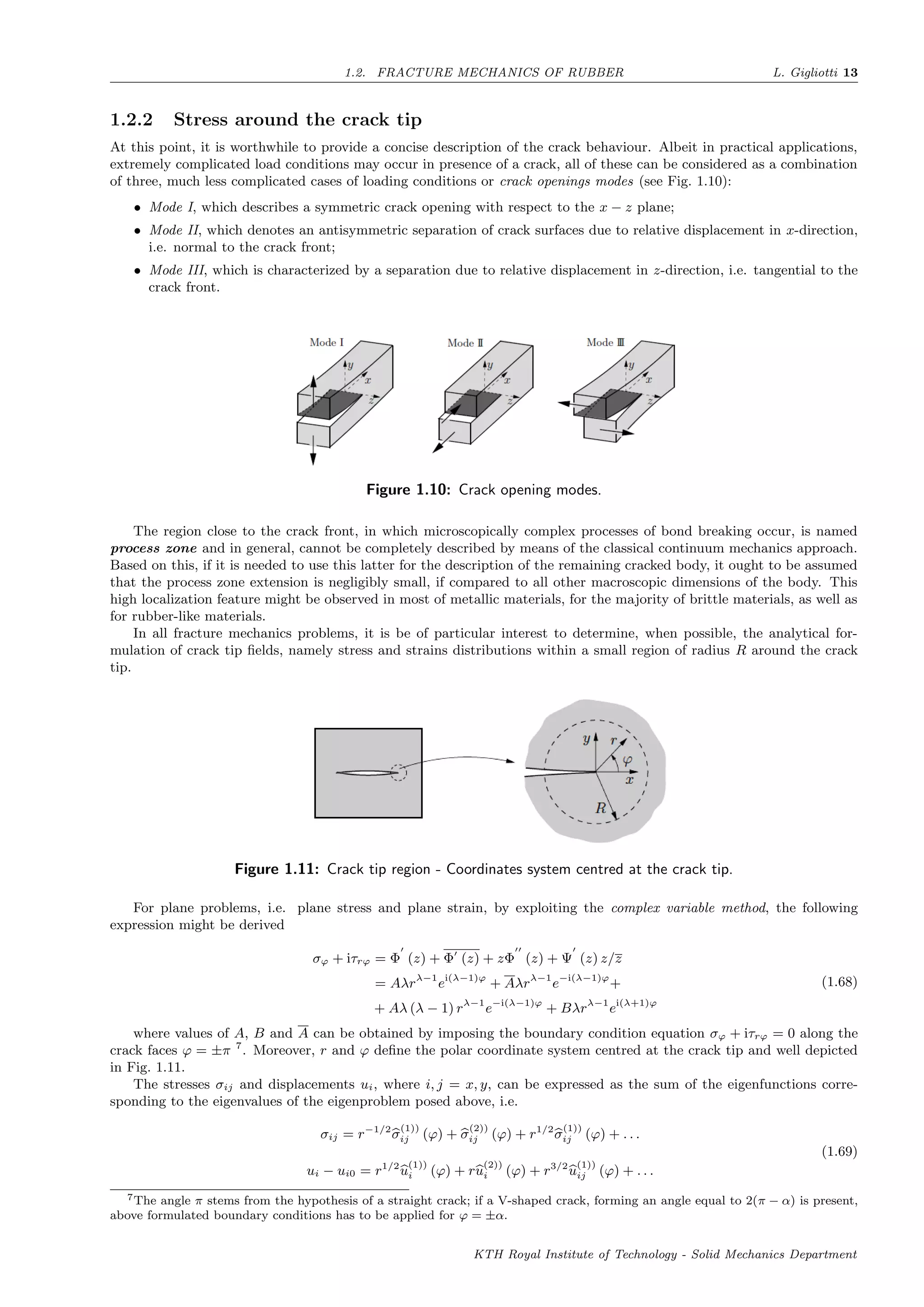
![14 L. Gigliotti CHAPTER 1. FUNDAMENTALS: LITERATURE REVIEW AND BASIC CONCEPTS
Here, ui0 represents an eventual rigid body motion while, for r → 0, the dominating term is the first one and thus
a singularity in the stress field is obtained at the crack tip. A widely adopted procedure is to split the symmetric sin-
gular field, corresponding to Mode-I crack opening, from the antisymmetric one, related to the Mode-II crack opening.
According to this latter consideration, stress and displacement fields at the crack tip for both Mode-I and Mode-II can
be written as follows
Mode-I :
σx
σy
τxy
= KI√
2πr
cos (ϕ/2)
1 − sin(ϕ/2) sin(3ϕ/2)
1 + sin(ϕ/2) sin(3ϕ/2)
sin(ϕ/2) cos(3ϕ/2)
u
v
= KI
2G
r
2π
(κ − cos (ϕ))
cos(ϕ/2)
sin(ϕ/2)
(1.70)
Mode-II :
σx
σy
τxy
= KII√
2πr
− sin(ϕ/2)[2 + cos(ϕ/2) cos(3ϕ/2)]
sin(ϕ/2) cos(ϕ/2) cos(3ϕ/2)
cos(ϕ/2)[1 − sin(ϕ/2) sin(3ϕ/2)]
u
v
= KII
2G
r
2π
sin(ϕ/2)[κ + 2 + cos(ϕ)]
cos(ϕ/2)[κ − 2 + cos(ϕ)]
(1.71)
where
plane stress : κ = 3 − 4ν, σz = 0
plane strain : κ = (3 − ν)/(1 + ν), σz = ν(σx + σy)
(1.72)
According to Eqs. 1.70 and 1.71, the amplitude of the crack tip fields is controlled by the stress-intensity factors
KI and KII ; their values depend on the geometry of the body, including the crack geometry, and on its load conditions.
Indeed, provided the stresses and deformations are known, it is possible to determine the K-values: for example, from
Eqs. 1.70 and 1.71 one might infer that
KI = limr→0
√
2πrσy (ϕ = 0) , and KII = limr→0
√
2πrτxy (ϕ = 0) (1.73)
In conclusion, it ought to be stressed that for larger distances from the crack tip, the higher terms in Eq. 1.69 cannot
be neglected and the effect of remaining eigenvalues has to be taken into account. Moreover, it has been observed that,
in most of the crack problems the characteristic stress singularity is of the order r−1/2
; however,different singularity
orders for the stress field might also come to light. As general remark, the stress singularities are of the type σij ∼ rλ−1
,
having denoted with λ the smallest eigenvalue in the eigenproblem formulated in Eq. 1.68.
1.2.3 Tearing energy
Theoretically, Griffith’s approach is suitable to predict the fracture mechanics behaviour of elastomers, since no limitations
to small strains or linear elastic material response have been made in its derivation. Many attempts have been carried
out throughout the years, to find a criterion for the crack propagation in rubber-like materials; however this task is
characterized by overwhelming mathematical difficulties in determining the stress field in a cracked body made of an
elastic material, due to large deformations at the crack tip prior failure. In addition, since high stresses developed are
bounded within a limited region surrounding the crack tip, their experimental measurements cannot be promptly carried
out.
Based on thermodynamic considerations, Griffith theory describes the quasi-static crack propagation as a reversible
process; on the other hand, for rubber-like materials the decrease of elastic strain energy is balanced not only by the
increase of the surface free energy of the cracked body, as hypothesized for brittle materials, but it is also partially
converted into other forms of energy, i.e. irreversible deformations of the material. Such other forms of dissipated energy
appear to be relevant only in proximity of the crack tip, i.e. in portions of material, relatively small if compared to the
overall dimensions of the component. It has been observed that, for a thin sheet of a rubber-like material, in which the
initial crack length is large if compared to its thickness, such energy losses are proportional to the rise of crack length.
In addition, they are readily computable just as function of the deformation state in the neighbourhood of the crack
tip at the tearing instant, while basically independent of the specimen type and geometry, and of the particular manner
in which the deforming forces are applied to the cracked body. Even if a slight dependence with the shape of the crack
tip is observed, such energy is a characteristic property of the tearing process of rubber-like materials.
Let us deform, under fixed-grip conditions, a thin sheet of rubber-like material cut by a crack of length a and whose
thickness is t. In order to observe the crack length increases of da, a work Tcr t da has to be done, where Tcr is the
critical energy for tearing and is a characteristic property of the material:
KTH Royal Institute of Technology - Solid Mechanics Department](https://image.slidesharecdn.com/5bffcdff-873e-4f02-b330-da222b639ff8-151115100138-lva1-app6891/75/FULLTEXT01-20-2048.jpg)
![1.2. FRACTURE MECHANICS OF RUBBER L. Gigliotti 15
Tcr = −
1
t
∂Us
∂a l
(1.74)
In the above expression, the suffix l indicates that the differentiation is performed with constant displacement of
the portions of the boundary which are not force-free. Physically, the critical energy for tearing Tcr represents the
whole dissipated energy as result of fracture propagation (of which, in certain cases, surface tension may be a minor
component). Therefore, this critical energy has to be compared with the tearing energy calculated from the deformation
state at the crack tip and whose value, as function of the notch tip diameter d is written as
T = d
π
2
0
U0
s cos (θ) dθ (1.75)
where, the term U0
s is the strain energy density at the notch tip for θ = 0.
Lastly, if the average strain energy density Ub
s is introduced, Eq. 1.75 is simplified as follows
T ∼= d Ub
s (1.76)
where the linear correlation of T with the notch diameter d is proven.
Concerning the physical meaning of Ub
s , this can be interpreted as the energy required to fracture a unit volume under
simple tension conditions and therefore, it is an intrinsic material property.
1.2.4 Qualitative observation of the tearing process
In [21], a formidable number of experiments have been carried out, in order to assess the effectiveness of the tearing
criterion expressed in Eq. 1.74; further information regarding vulcanizate materials adopted and experimental modalities
are given in the cited work. Irreversible behaviour is observed exclusively within the neighbourhood region of the crack
tip, where the material undergoes large deformations; in addition, if experimental tests are performed at a sufficiently
slow rate of deformation, these are not affected by the test speed.
To present a qualitative description of the tearing process, we may now consider a thin sheet of vulcanizate in which a
pre-existent crack is present. Experimental observations show how, even relatively small forces lead to considerable values
of the tearing energy and, in addition, the tearing process ceases as soon as the deformation process is interrupted. The
crack propagation process can be readily described since its earlier stages: as the deformation continues, the crack grows
up to a few hundredths of millimetres. Once this condition is reached, catastrophic failure occurs and the crack length
abruptly grows by a few millimetres. Such propagation mechanism is repeated as the deformation further increases,
leading to a catastrophic rupture of the cracked body.
As always, in fracture mechanics analysis, noticeable information might be deduced from the observation of the crack
tip geometry. In the process of crack growth in elastomers, during the stages preceding the catastrophic rupture, the
crack tip is initially blunted, whilst, as the tragic rupture occurs, the crack tip assumes an increasingly irregular shape.
Last but not least, it has to be stressed that the instant at which the catastrophic rupture commences, is by definition,
taken as the tearing point.
1.2.5 Tearing energy for different geometries
1.2.5.1 The trousers test-piece
The trousers specimen (see Fig. 1.12) has been widely used for the determination of out-of-plane mode-III critical tearing
energy for elastomers. Historically, is one of the first specimens introduced for the determination of fracture properties
of elastomers.
Figure 1.12: Trousers test-piece.
The energy balance in the specimen might be written as
∂W
∂a
=
∂T
∂a
+
∂Us
∂a
(1.77)
KTH Royal Institute of Technology - Solid Mechanics Department](https://image.slidesharecdn.com/5bffcdff-873e-4f02-b330-da222b639ff8-151115100138-lva1-app6891/75/FULLTEXT01-21-2048.jpg)
![16 L. Gigliotti CHAPTER 1. FUNDAMENTALS: LITERATURE REVIEW AND BASIC CONCEPTS
where W is the work done by the applied forces, T is the energy required for tearing and Us is the total internal
strain energy.
Next, assuming that the stretch ratio λ in the specimen, whose thickness is indicated with t and the width with w,
is equal to λ = 1 + (u/L) ≥ 1 under the applied force F, Eq. 1.77 can be reformulated as follows
2Fλ = Tt + Ψwt (1.78)
In addition, since λ = 1 in the reference configuration, according to the normalization condition, the strain energy
Ψ vanishes; therefore, the following expression of the tearing energy T may be inferred
T =
2F
t
(1.79)
showing the linear dependence of the tearing energy on the applied force F.
1.2.5.2 The constrained tension (shear) specimen
This specimen, also called pure shear test-piece [28], is constituted of a long strip of (rubber-like) materials which contains
a symmetrically located cut (see Fig. 1.13). Let the strip be clamped along its parallel sides, and make them move apart
of a distance v0 in the y-direction, in correspondence of which the material starts to crack and then held at this position.
Figure 1.13: Constrained tension (shear) specimen.
If both the strip and the crack are sufficiently long, three different regions are distinguished, namely:
• Region 1, which remains unstressed and whose related strain energy U1
s vanishes;
• Region 2, the region containing the crack-tip and in which the strain energy U2
s is an unknown complicated function
of x and y;
• Region 3, characterized by an uniform stress distribution and within which, the strain energy U3
s = U0
s is constant.
The constant strain energy U0
s might be computed as function of the relative clamp displacement v0 and of constitutive
material properties. At this point, it is worthwhile remarking on that, as the crack propagates by a certain length da,
Region 2 simply moves with the crack tip while the strain energy value U2
s remains constant. In other words, the
extension of the unstressed Region 1 grows whereas contemporary, Region 2 becomes larger as the crack propagates.
The net variation of the overall strain energy Us is given by
dUs = −U0
s h t da (1.80)
By virtue of Eq. 1.74, together with Eq. 1.80, the expression of the tearing energy expression in the case of constrained
tension (shear) specimen is obtained
T = −
1
t
∂Us
∂a l
= U0
s h (1.81)
1.2.5.3 The tensile strip specimen
Another well-known specimen adopted for the characterization of fracture mechanics properties of rubber-like materials,
is the tensile strip specimen. This specimen, consists in a thin sheet of rubber, containing a crack, whose length a is
small if compared to the length L of the test piece. The strain distribution in a small region surrounding the crack tip
is inhomogeneous, while in the center of the sheet, far from the crack tip, the specimen might be reasonably assumed to
be in simple extension conditions. In addition, the region indicated in Fig. 1.14 on the next page with A, namely the
area at the intersection of the cut and the free edge of the specimen, results to be unstretched.
Given the complexity of the strain distribution around the crack tip, in [21] dimensional considerations allow us to
state that, if a test piece is cut by an ideally sharp crack in its undeformed configuration, the variation in the elastically
stored energy due to its presence, will be proportional to a2
. Such evidence is strictly valid only for ideally sharp crack
and semi-infinite sheet, but it can be easily extended for other practical cases, provided that the radius of curvature at
the notch is small if compared with the crack length a. The variation of such elastically stored energy, caused by the
introduction of the crack in the specimen is expressed by the following relation
KTH Royal Institute of Technology - Solid Mechanics Department](https://image.slidesharecdn.com/5bffcdff-873e-4f02-b330-da222b639ff8-151115100138-lva1-app6891/75/FULLTEXT01-22-2048.jpg)
![1.2. FRACTURE MECHANICS OF RUBBER L. Gigliotti 17
Figure 1.14: Tensile strip specimen with a crack of length a.
Us − Us = k a2
t (1.82)
where the elastically stored energy in the absence of the crack is denoted by Us and the constant of proportionality
k is function of the extension rate λ. The proportionality between Us − Us and the thickness t holds only if plane stress
conditions are employed, i.e. t a.
At this point, it is straightforward to observe that, given the proportionality of the specimen elongation with λ − 1,
the energy variation Us −Us will be proportional to (λ−1)2
or, in other words, to the strain energy density Ψ. By virtue
of the above considerations, Eq. 1.82 can be reformulated as
Us − Us = ka2
tΨ (1.83)
where k is a function of λ.
By differentiating Eq. 1.83 with respect to the crack length a, finally the expression of the tearing energy for the
tensile strip specimen get the form
−
∂Us
∂a l
= 2kΨat ⇒ T = −
1
t
∂Us
∂a l
= 2kΨa (1.84)
Concerning the dependance of the constant k with the extension rate λ, several experiments and FEA simulations
have been performed [30, 31] showing the proportionality of k with the inverse of the square root of λ, through the
constant π, i.e.
k =
3
√
λ
(1.85)
Although the three test specimens presented so far, are widely used in experimental procedures, compression and
shear are encountered much more often in engineering applications, because under these load conditions rubber-like
materials can be fully used without risks of crack growth.
1.2.5.4 The simple shear test-piece
A mathematically simple expression for the tearing energy T in simple shear specimens (see Fig. 1.15) has the form
T = kΨh (1.86)
Figure 1.15: Simple shear test-piece with an edge crack.
KTH Royal Institute of Technology - Solid Mechanics Department](https://image.slidesharecdn.com/5bffcdff-873e-4f02-b330-da222b639ff8-151115100138-lva1-app6891/75/FULLTEXT01-23-2048.jpg)
![18 L. Gigliotti CHAPTER 1. FUNDAMENTALS: LITERATURE REVIEW AND BASIC CONCEPTS
In such case, the constant of proportionality k, commonly assumes the value of 0.4, but its range of variation is
between 0.2 and 1.0, depending on the configuration and size of the crack. In practical situations, it is really demanding
to carry out simple shear experiments since, as the crack grows, it tends to change direction to Mode-I crack opening. In
addition, relation Eq. 1.80 holds only if the crack is short, and this implies difficulties in the determination of the stress
concentration.
1.2.5.5 The uniaxial compression test piece
Uniaxial compression specimen slightly differs from those discussed in the previous sections; indeed, the strain distribution
is highly inhomogeneous even without cracks within the component. For the strain energy Ψ of such test-piece, provided
strains are often small enough, the following linear approximation holds
Ψ =
1
2
Ece2
c (1.87)
where e2
c is the compressive strain, while the compression modulus Ec is defined as
Ec = 2G 1 + 2S2
(1.88)
where G is the small strain shear modulus.
The factor S in Eq. 1.88 referred to as a shape factor, is the ratio between the loaded area and the force-free
surface, i.e.
S =
πD2
/4
πDh
=
D
4h
(1.89)
According to [29], when a bonded rubber unit is cyclically loaded in compression, an approximately parabolic surface
is generated and the crack initiates at the intersection of such surface with the core of the specimen (see Fig. 1.16)
Figure 1.16: Typical stages of crack growth in compression: a) unstrained b) compressed - crack
initiation at bond edges c) compressed - bulge separate from core d) unstrained - showing parabolic
crack locus.
Under these assumptions, the tearing energy for uniaxial compression test-piece is given by the approximated ex-
pression, valid for S > 0.5 and strains below 50%
T =
1
2
Ψh =
1
4
Ece2
ch (1.90)
1.3 eXtended Finite Element Method
1.3.1 Introduction
Results presented in the previous section, concerning the analytical treatments of fracture mechanics problems are
affected by certain limitations, among which the most constraining are undoubtedly the following ones:
• The material domain is always considered infinite, in order to neglect edge effects in the mathematical derivation
of stress and displacement distributions;
• In the majority of cases, the material is assumed to be homogeneous and isotropic;
• Only simple boundary conditions are considered.
However, it is easy to guess that in practical problems of complex structures, containing defects of finite sizes, subject
to complicated boundary conditions and whose material properties are much more complicated than those related to the
ideal linear, homogeneous and isotropic material model, a satisfactory fracture mechanics analysis can be carried out
exclusively by means of numerical methods. Among these, the most widely adopted in practical engineering applications
is the finite element method [33]; for this reason, several software packages based on the FEM technique have been
developed throughout the years [34]. Although the finite element method has shown to be particularly well-suited for
fracture mechanics problems [35, 36, 37], the non-smooth crack tip fields in terms of stresses and strains can be captured
KTH Royal Institute of Technology - Solid Mechanics Department](https://image.slidesharecdn.com/5bffcdff-873e-4f02-b330-da222b639ff8-151115100138-lva1-app6891/75/FULLTEXT01-24-2048.jpg)
![1.3. EXTENDED FINITE ELEMENT METHOD L. Gigliotti 19
only by a locally refined mesh. This leads to an abrupt increase of the number of degrees of freedom and such defect is
worsened in 3D-problems. Concerning the crack propagation analysis, it still remains a challenge for several industrial
modelling problems. Indeed, since it is required to the FEM discretization to conform the discontinuity, for modelling
evolving discontinuities, the mesh has to be regenerated at each time step. This means that the solution has to be re-
projected for each time step on the updated mesh, causing a dramatic rise in terms of computational costs and to a loss
of the quality of results [38]. Because of these limitations, several numerical approaches to analyze fracture mechanics
problems have been proposed during last years. The method based on the quarter-point finite element method [39], the
enriched finite element method [40, 41], the integral equation method [42], the boundary collocation method [43], the
dislocation method [44, 45], the boundary finite element method [46], the body force method [47] and mesh-free methods
[48, 49], e.g. free-element Galerkin method [50, 51], represent the most valuable examples. In order to overcome the need
of remeshing, different techniques have been introduced over the last decades, e.g. the incorporation of a discontinuous
mode on an element level [52], a moving mesh technique [53] and an enrichment technique, based on the partition of
unity, later referred to as the eXtended Finite Element Method (XFEM) [54, 56, 55].
1.3.2 Partition of unity
Given a C∞
manifold M, with an open cover Ui, a partition of unity subject this latter, is a collection of n nonnegative,
smooth functions fi such that, their support is included in Ui and the following relation holds
n
i=1
fi(x) = 1 (1.91)
Often it is required that, the cover Ui have compact closure, which can be interpreted as finite, or bounded, open
sets. If this condition is locally verified, any point x in M has only finitely many i with fi(x) = 0. It can be easily
demonstrated that, the sum in Eq. 1.91 does not have to be identically unity to work; indeed, for any arbitrary function
ψ(x) it is verified that
n
i=1
fi(x)ψ(x) = ψ(x) (1.92)
Furthermore, it might be inferred that the partition of unity property is also satisfied by the set of isoparametric
finite element shape functions Nj. i.e.
m
j=1
Nj(x) = 1 (1.93)
1.3.2.1 Partition of unity finite element method
To increase the order of completeness of a finite element approximation, the so-called enrichment procedure may be
exploited. In other words, the accuracy of solution can be ameliorated, by simply including in the finite element
discretization, the a priori analytical solution of the problem. For instance, in fracture mechanics problems, an improve-
ment in predicting crack tip fields is achieved, if the analytical crack tip solution is included in the framework of the
isoparametric finite element discretization. Computationally, this involves an increase in number of the nodal degrees of
freedom.
The partition of unity finite element method (PUFEM) [57] [58], using the concept of enrichment functions along
with the partition of unity property in Eq. 1.93, allows to obtain the following approximation of the displacement within
a finite element
uh
(x) =
m
j=1
Nj(x) uj +
n
i=1
pi(x)aji (1.94)
where, pi(x) are the enrichment functions and aji are the additional unknowns or degrees of freedom associated to
the enriched solution. With m and n the total number of nodes of each finite element and the number of enrichment
functions pi, are indicated.
By virtue of Eqs.1.92 and 1.93, for an enriched node xk, Eq. 1.94 might be written as
uh
(xk) = uk +
n
i=1
pi(xk)aji (1.95)
which is clearly not a plausible solution. To overcome this defect and satisfy interpolation at nodal point, i.e.
uh
(xi) = ui, a slightly modified expression for the enriched displacement field is proposed below
uh
(x) =
m
j=1
Nj(x) uj +
n
i=1
(pi(x) − pi(xj)) aji (1.96)
KTH Royal Institute of Technology - Solid Mechanics Department](https://image.slidesharecdn.com/5bffcdff-873e-4f02-b330-da222b639ff8-151115100138-lva1-app6891/75/FULLTEXT01-25-2048.jpg)
![20 L. Gigliotti CHAPTER 1. FUNDAMENTALS: LITERATURE REVIEW AND BASIC CONCEPTS
1.3.2.2 Generalized finite element method
A breakthrough in increasing the order of completeness of a finite element discretization is provided by the so-called
generalized finite element method (GFEM) [59, 60], in which two separate shape functions are employed for the ordinary
and for the enriched part of the finite element approximation, i.e.
uh
(x) =
m
j=1
Nj(x)uj +
m
j=1
Nj(x)
n
i=1
pi(x)aji (1.97)
where Nj(x) are the shape functions associated with the enrichment basis functions pi(x).
For the reason explained in the previous section, Eq. 1.97 should be modified as follows
uh
(x) =
m
j=1
Nj(x)uj +
m
j=1
Nj(x)
n
i=1
(pi(x) − pi(xj)) aji (1.98)
1.3.3 eXtended Finite Element Method
The eXtended Finite Element Method is a partition of unity based method in which, as for PUFEM and GFEM, the
classical finite element approximation is enhanced by means of enrichment functions. However, in PUFEM and GFEM,
the enrichment procedure involves the entire domain, whilst it is employed on a local level for the XFEM. Thus, only
nodes close to the crack tip, as well as the ones required for the correct localization of the crack, are enriched. This
evidently entails a tremendous computational advantage.
The XFEM method was firstly introduced by Belytsckho and Black in 1999 [61]. Their work, in which a method for
enriching finite element approximation in such a way that crack growth problems can be solved with minimal remeshing,
represents a milestone in the XFEM history. Later on, much more elegant formulations, including the asymptotic near-tip
field and the Heaviside function H(x) in the enrichment scheme, have been proposed [62, 63, 64]8
. The eXtended Finite
Element method, furthermore, has been demonstrated to be well suited for three dimensional crack modelling [65]. In
this latter work, geometric issues associated with the representation of the crack and the enrichment of the finite element
approximation have been addressed. A major step forward has been then achieved when a generalized methodology for
representing discontinuities, located within the domain indipendetely from the mesh grid, has been proposed [66, 62]. In
such manner, the eXtended Finite Element Method allows to alleviate much of the burden related to the mesh generation,
as the finite element mesh is not supposed to conform the crack geometry anymore. This represents certainly, one of the
major advantages provided by the XFEM usage. The XFEM capabilities can be extended if employed in conjunction
with the Level Set Method (LSM) [67, 68, 69]. Such method permits to represent the crack position, as well as the
location of crack tips. Within this context, the XFEM has also been employed in concert with a particular type of level
set method named Fast Marching Method [70, 71]. Accuracy, stability and convergence of XFEM, along with difficulties
in using the standard Gaussian quadrature have been investigated [72, 73]; a solution to this latter drawback has been
proposed in [74].
1.3.3.1 Enrichment functions
In two-dimensional problems, crack modelling is obtained by means of two different types of enrichment functions:
• The Heaviside function
The Heaviside function H(x), is employed to enrich elements completely cut by the crack. The splitting of the
domain by the crack, causes a jump in the displacement field and the Heaviside function provides a tremendously
simple mathematical tool to model such behaviour.
Given a continuous curve Γ, representing a crack within the deformable body Ω, let us consider a point x (x, y) ∈ Ω.
The whole aim is to determine the position of such point with respect to the crack location. In this context, if the
closest point belonging to Γ is denoted with x (x, y) and the outward normal vector to Γ in x with n (see Fig. 1.17
on the facing page), the Heaviside function might be defined as follows
H (x, y) =
1 for (x − x) · n > 0
−1 for (x − x) · n < 0
(1.99)
If no unique normal is defined, then the H(x) function will assume a positive value if (x − x) belong to the con of
normals in x (see Fig. 1.17 on the next page)
• Asymptotic near-tip field functions
In case of not completely cracked element, the Heaviside function cannot be used to approximate the displacement
field over the entire element domain, since the element contains the crack tip. In [51] it has been proven that
the displacement field from LEFM theory in Eqs. 1.70 and 1.71, is included within the span of the following four
functions, expressed in terms of the local crack tip coordinate system (r, θ)
{Fi(r, θ)}4
i=1 =
√
r cos θ
2
,
√
r sin θ
2
,
√
r sin θ
2
sin (θ)
√
r cos θ
2
sin (θ) (1.100)
8In [64], the name eXtended Finite Element Method has been used for the first time.
KTH Royal Institute of Technology - Solid Mechanics Department](https://image.slidesharecdn.com/5bffcdff-873e-4f02-b330-da222b639ff8-151115100138-lva1-app6891/75/FULLTEXT01-26-2048.jpg)
![1.3. EXTENDED FINITE ELEMENT METHOD L. Gigliotti 21
(a) Smooth crack. (b) Kink crack.
Figure 1.17: Evaluation of the Heaviside function.
By using the enrichment functions in Eq. 1.100, four different additional degrees of freedom in each direction
for each node are added to those related to the standard finite element discretization. It should be stressed that
among the aforementioned enriching functions (see Fig. 1.18), only the second term
√
r sin θ
2
is discontinuous
along crack surfaces and hence, is responsible of the discontinuity in the approximation along the crack. The
remaining three functions are used to enhance the solution approximation in the neighborhood of the crack tip.
(a)
√
r cos θ
2
. (b)
√
r sin θ
2
.
(c)
√
r sin θ
2
sin (θ). (d)
√
r cos θ
2
sin (θ)
Figure 1.18: Near-tip enrichment functions.
Lastly, it should be highlighted that, referring to Eq. 1.100, the required singularity in the stress field, of order
1√
r
is, therefore, readily introduced.
By virtue of the above discussed enrichment functions, the following expression for the XFEM approximation might
be formulated
uh
(x) = uF EM (x) + uENR (x) =
=
i∈I
Ni (x) ui +
j∈J
Nj [H (x)] aj +
k∈K1
Nk (x)
4
l=1
bl1
k F1
l (x) +
+
k∈K2
Nk (x)
4
l=1
bl2
k F2
l (x)
(1.101)
or, to eliminate the lack of interpolation property
KTH Royal Institute of Technology - Solid Mechanics Department](https://image.slidesharecdn.com/5bffcdff-873e-4f02-b330-da222b639ff8-151115100138-lva1-app6891/75/FULLTEXT01-27-2048.jpg)
![22 L. Gigliotti CHAPTER 1. FUNDAMENTALS: LITERATURE REVIEW AND BASIC CONCEPTS
uh
(x) =
i∈I
Ni (x) ui +
j∈J
Nj [H (x) − H (xj)] aj +
+
k∈K1
Nk (x)
4
l=1
bl1
k F1
l (x) − F1
l (xk) +
k∈K2
Nk (x)
4
l=1
bl2
k F2
l (x) − F2
l (xk)
(1.102)
where, J indicates the set of nodes whose support domain is completely cut by the crack and thus enriched with
the Heaviside function H (x), K1 and K1 are the sets of nodes associated with the crack tips 1 and 2 in their influence
domain, respectively, and whose respective crack tip enrichment functions are F1
l (x) and F2
l (x). Moreover, ui are
the standard degrees of freedom, while aj, bl1
k and bl2
k indicate the vectors of additional nodal degrees of freedom for
modelling crack faces and the two crack tips, respectively.
1.3.3.2 Level set method for modelling discontinuities
In several cases, numerical simulations involve time-varying objects, like curves and surfaces on a fixed cartesian grid, e.g.
interfaces, discontinuities, etc. Their modelling and tracking is particularly cumbersome and is based on the complex
mathematical procedure denominated parametrization.
The Level Set Method [68] (often abbreviated as LSM) is an elegant numerical technique that allows to get over
these difficulties. The key-point of such method is to represent discontinuities as a zero level set function. For this
purpose, to fully characterize a crack, two different level set functions are defined
1. A normal level set function, ϕ (x)
2. A tangential level function, ψ (x).
At this point, for the evaluation of the signed distance functions, let Γc be the crack surface (see Fig. 1.19) and x the
point in which it is sought to evaluate the ϕ (x) function. In an analogous manner of what done in the foregoing section,
the normal level set function might be defined as
ϕ = (x − x) · n (1.103)
where x and n assume the previously stated meanings (see Fig. 1.17 on the preceding page) 9
.
Figure 1.19: Construction of level set functions.
In Fig. 1.20 on the next page, the plot of the normal signed function ϕ (x) for an interior crack is provided.
The tangential level set function ψ (x) is computed by finding the minimum signed distance to the normal at the
crack tip; in case of an interior crack, two different functions can be individuated. However, a unique tangential level set
function can be defined as
ψ (x) = max {ψ1 (x) , ψ2 (x)} (1.104)
In conclusion, referring to Fig. 1.19, it may be written what follows
for x ∈ Γcr ϕ (x = 0) and ψ (x ≤ 0)
for x ∈ Γtip ϕ (x = 0) and ψ (x = 0)
(1.105)
9According to the definition given in Eq.1.103, in case of interior crack, the normal level set function is computable only within
the region delimited by the normals to the crack tips; in order to define ϕ (x) over the whole domain, both crack tips should be
virtually extended.
KTH Royal Institute of Technology - Solid Mechanics Department](https://image.slidesharecdn.com/5bffcdff-873e-4f02-b330-da222b639ff8-151115100138-lva1-app6891/75/FULLTEXT01-28-2048.jpg)
![1.3. EXTENDED FINITE ELEMENT METHOD L. Gigliotti 23
(a) 2D contour of ϕ (x). (b) 3D contour of ϕ (x).
Figure 1.20: Normal level set function ϕ (x) for an interior crack.
(a) 2D contour of ψ (x). (b) 3D contour of ψ (x).
Figure 1.21: Tangential level set function ψ (x) for an interior crack.
where Γtip indicates the crack tips location.
1.3.3.3 Blending elements
Discussing different methods exploiting the partition of unity property, e.g. PUFEM and GFEM, the advantage in
terms of computational cost related to the XFEM has been introduced. Indeed, unlike PUFEM and GFEM, in XFEM
the enriching functions are introduced only in a local part of the domain, in order to capture the non-smooth solution
characteristics. Elements, whose all nodes have been enriched are named reproducing elements since they allow to
reproduce the enrichment functions exactly. Besides these, there are the so-called blending elements, whose role is to
blend the enriched sub-domain with the rest of the domain, where, being the solution smooth, standard (not enriched)
finite elements are employed. Only some of nodes in blending elements are enriched. Enriched finite elements, blending
elements and standard finite elements partition the whole domain in three different parts, an enriched domain, a blending
domain and a standard domain, respectively, as shown in Fig. 1.22 on the next page.
Two important drawbacks affect blending elements, i.e.
• Enrichment functions cannot be reproduced exactly in blending elements, since the partition of unity property is
not satisfied within them;
• These elements produce unwanted terms in the approximation, which cannot be compensated by the FE part; for
instance, if the enrichment introduces non-linear terms, a linear function can no longer be approximated within
blending elements.
Unlike the first one, which does not represent a dramatic problem in the XFEM, the second drawback implies a
significant reduction of the convergence rate for general enrichment functions [72]; thus, suboptimal rate of convergence
in XFEM may be caused by problems in blending elements [73]. A relatively straightforward method to circumvent
this defect is to exploit a blending ramp function R over the transition region connecting domains with and without
enrichment, i.e.
uh
(x) = uF EM
(x) + RuENR
(x) (1.106)
KTH Royal Institute of Technology - Solid Mechanics Department](https://image.slidesharecdn.com/5bffcdff-873e-4f02-b330-da222b639ff8-151115100138-lva1-app6891/75/FULLTEXT01-29-2048.jpg)
![24 L. Gigliotti CHAPTER 1. FUNDAMENTALS: LITERATURE REVIEW AND BASIC CONCEPTS
Figure 1.22: Standard, enriched and blending elements.
where R is set equal to 1 on the enrichment boundary, and equal to 0 on the standard finite element discretization
boundary. This linear blending function R ensures the continuity in the displacement field but not in the strain field. To
achieve this latter, higher order blending functions should be used. Other approaches prescribe to use enhanced strain
techniques or p-refinement in blending elements [75], or to adjust the order of the FE shape functions depending on the
enrichment [76]. Recently, an interesting solution has been proposed in [77]; in particular, in this work the enrichment
functions have been modified such that they vanish in standard elements, unchanged in elements with all their nodes
being enriched and continuously varying within blending elements. In such approach all nodes of blending elements are
enriched.
1.3.3.4 XFEM discretization
Consider a regular region Ω bounded by a smooth curve ∂Ω in the reference configuration, and let this latter be split
in two portions, namely ∂Ωt and ∂Ωu. Essential boundary conditions are imposed on ∂Ωu while traction boundary
conditions are applied along ∂Ωt. Let the region Ω be cut by a crack, whose surfaces ∂Ωcr are traction free. The strong
form of the initial boundary value problem can be written as
DivP + Bf = ρ0¨u in Ω
u = u on ∂Ωu
PN = o on ∂Ωcr
PN = T on ∂Ωt
(1.107)
where Bf and ρ0¨u denote the reference body force and the inertia force per unite reference volume, respectively, N
the outward unit normal to ∂Ω, u the prescribed displacement vector and T the prescribed first Piola-Kirchhoff traction
vector.
The displacement field u must satisfy all the essential boundary conditions and the smoothness property, so that u
is continuous C0
in Ω, i.e.
u ∈ U, U = u|u ∈ C0
except on ∂Ωcr , u = u on ∂Ωu (1.108)
At the same time, test functions δv are defined by
δv ∈ U0, U0 = δv|δv ∈ C0
except on ∂Ωcr , δv = 0 on ∂Ωu (1.109)
Thus, using the above concepts, the weak form of the equilibrium equation and traction boundary conditions might
be formulated as
Ω
S : δE dV =
Ω
(Bf − ρ0¨u) · δu dV +
∂Ωt
T · δu dA (1.110)
In engineering problems, the nonlinear boundary-value problem in Eq. 1.110 is numerically solved by means of
the iterative procedure known as Newton-Raphson method. The main idea behind such method is to linearize all
quantities associated with the problem at hand, replacing it with a series of linear problems, whose resolution is much
more undemanding. The linearization procedure is the foundation of finite element methods [33, 78]. Here we present the
XFEM discretization of problem in Eq. 1.110 for the particular case of hybrid elements and incompressible hyperelastic
material model. Hybrid elements use the well-known in computational mechanics field Hu-Washizu mixed form [79, 80].
The resulting elements exhibit the capabilities to overcome the locking effects. In such elements the strain and/or stress
field is interpolated independently of the displacement field. The utilization of mixed forms is particularly profitable
for constrained problems. In addition, the incompressibility constrained is modeled by making use of the Lagrange
multipliers (Cfr. Sec. 1.1.2.2).
The resulting linearized equations, may be expressed as follows
KTH Royal Institute of Technology - Solid Mechanics Department](https://image.slidesharecdn.com/5bffcdff-873e-4f02-b330-da222b639ff8-151115100138-lva1-app6891/75/FULLTEXT01-30-2048.jpg)
![1.3. EXTENDED FINITE ELEMENT METHOD L. Gigliotti 25
J GT
G 0
δuh
δp
=
−rv − GT
pv
−GT
∆u
h
v
(1.111)
In the above matrix relation, the Jacobian matrix J, and the matrix G can be respectively written as
J =
sD
β∆t2
M + Kint
+ Kext
, G =
∂g
∂u
(1.112)
We first consider the J matrix. In the first term on the RSH, which is present only in dynamic problems, β is the
parameter of the Newmark β-method, M is the mass matrix and ∆t is the time step increment. The second and the
third term are respectively the tangent stiffness matrices for internal and external nodal forces; this latter can be
easily expressed as Kext
= ∂fext
∂u
.
In the supposition that only one crack tip is present within the body, the vector of nodal parameters uh
is defined
as follows
uh
= {u a b1 b2 b3 b4}T
(1.113)
Concerning the global tangent stiffness matrix for internal forces Kint
and the global vector of external forces fext
,
these are obtained by assembling the tangent stiffness matrix for internal forces Kint e
ij and the vector of external forces
fext e
i for each element e of the XFEM discretization, i.e.
Kint e
ij =
Kuu
ij Kua
ij Kub
ij
Kau
ij Kaa
ij Kab
ij
Kbu
ij Kba
ij Kbb
ij
(1.114)
fext e
i = fu
i fa
i fb1
i fb2
i fb3
i fb4
i
T
(1.115)
with
Krs
ij =
Ωe
[(Br
i )T
: CSE
: Bs
j + I(Br
i )T
: (S − pC−1
) : Bs
j ]dΩ , r, s = u, a, b (1.116)
fu
i = ∂Ωe
t
Nift
dA + Ωe
t
Nifb
dV
fa
i = ∂Ωe
t
NiHft
dA + Ωe
t
NiHfb
dV
fbα
i = ∂Ωe
t
NiFαft
dA + Ωe
t
NiFαfb
dV , α = 1, 2, 3 and 4
(1.117)
In Eq. 1.116, CSE
is a forth order tensor often referred to as tangent modulus tensor defined through the relation
˙S = CSE
: ˙E, while B is the shape function derivatives matrix, i.e.
Bu
i =
Ni,x 0
0 Ni,y
Ni,y Ni,x
(1.118)
Ba
i =
[Ni(H(ξ) − H(ξi))],x 0
0 [Ni(H(ξ) − H(ξi))],y
[Ni(H(ξ) − H(ξi))],y [Ni(H(ξ) − H(ξi))],x
(1.119)
Bb
i = Bb1
i Bb2
i Bb3
i Bb4
i
Bbα
i =
[Ni (Fα − Fαi)],x 0
0 [Ni (Fα − Fαi)],y
[Ni (Fα − Fαi)],y [Ni (Fα − Fαi)],x
, α = 1, 2, 3 and 4
(1.120)
where ξ is the local curvilinear (mapping) coordinate system. In addition, B represents the column matrix of
derivatives of shape functions I given by [B]iI = ∂NI
∂xi
in the reference configuration.
Furthermore, in Eq. 1.111, p is the Lagrangian multipliers vector, δuh
is the incremental displacement in the iterative
Newton procedure, ∆uh
the step increment and δp the virtual pressure field. Concerning the Lagrange multipliers
method, G is the matrix of material derivatives of constraints, i.e. G = ∂g
∂u
. In conclusion, r is the residual column
matrix and the subscript v represent the iteration number. In this formulation the Lagrange multiplier p can be regarded
as the physical hydrostatic pressure.
The above discussed formulation leads to a two-fields mixed finite element implementation in which the displacement
field and the hydrostatic pressure are treated as independent field variables. Lastly, it is fundamental to highlight
that such formulation requires to consider an additional numbers of unknown, i.e. equal to the number of Lagrange
multipliers sought. Along with the additional DOFs introduced by the XFEM technique, this renders the treatment of
incompressible materials with such method, extremely costly from a computational perspective.
KTH Royal Institute of Technology - Solid Mechanics Department](https://image.slidesharecdn.com/5bffcdff-873e-4f02-b330-da222b639ff8-151115100138-lva1-app6891/75/FULLTEXT01-31-2048.jpg)
![26 L. Gigliotti CHAPTER 1. FUNDAMENTALS: LITERATURE REVIEW AND BASIC CONCEPTS
1.3.3.5 Numerical integration and convergence
Though the Gauss quadrature has been proven to be exact for polynomial integrands, for non-polynomial ones it may
cause a reduction in the accuracy of results. Introducing an arbitrary oriented discontinuity in the finite element
discretization transforms displacements and stresses into highly non-linear fields which cannot be correctly integrated.
To circumvent such problems, a subtriangulation procedure (see Fig. 1.23), in which elements edges conform the crack
faces has been proposed [62]; within these elements the standard Gauss integration procedure might be exploited.
Figure 1.23: Subtriangulation of elements cut by a crack.
It has to be highlighted that, for elements containing the crack, therefore including the singular stress field at the
crack tip, this procedure might result to be inaccurate if Gauss points of sub-triangles are too close at the crack tip.
Crack modeling with the standard finite element method, is performed by re-meshing the domain so that elements
boundaries match the crack geometry; furthermore, new created elements have to be well conditioned and not badly
shaped. Accordingly, re-meshing procedure is a cumbersome and computationally costly operation. On the contrary,
since the sub-triangulation is performed only for integration purposes, no additional degrees of freedom are added to the
system and, sub-triangles are not forced to be well shaped.
It is worth mentioning that an alternative method based on the elimination of quadrature sub-elements has been
recently proposed [74]. In such approach, rather then partition elements cut by a crack, discontinuous non-differentiable
functions are replaced with equivalent polynomial functions and consequently the Gauss quadrature can be carried out
over the whole element. Although this method would allow a sensible reduction in terms of computational costs, it is
still affected by some drawbacks, e.g. it is limited to element completely cut by a straight crack, no additional rules
are prescribed for elements containing the crack tip and even if the solution is accurate for triangular and tetrahedral
elements, difficulties are still encountered in dealing with quadrilateral elements.
In conclusion, as previously stated, the XFEM method ensures more accurate results than classical FEM one.
However, the rate of convergence does not improve as the mesh parameter h goes to zero due to the presence of the
singularity [73] and it is lower than the one expected by using the classical FEM method in smooth problems10
. Several
methods have been proposed during last decades to achieve an optimal rate of convergence, e.g. XFEM with a fixed
enrichment area, high-order XFEM [72, 81] as well as a modified construction of blending elements. In [82] the robustness
of the method has been enhanced by means of a new integration quadrature for asymptotic functions and implementing
a preconditioning scheme adapted to enrichment functions.
1.3.3.6 XFEM for finite strain fracture mechanics
Numerical methods based of the Finite Element Method, devoted to the computational analysis of crack propagation
phenomena in non-linear fracture mechanics is still an open problem [83, 84].
Even more cumbersome is the application of the eXtended Finite Element Method to large strain problems; indeed,
very few works have been intended to extend the XFEM capabilities to materials exhibiting a nonlinear behaviour
and able to undergo large deformations, especially if associated with the volumetric incompressibility constraint. The
satisfaction of such constraint within the enriched approximation is thought to be, in this context, the most difficult
issue and requires to be further investigated. For this purpose, the enrichment of a standard biquadratic-displacement
bilinear pressure for node quadrilateral element has been proposed [85]. Nevertheless, even if very good results have been
achieved in terms of stress and displacement fields prediction, the extent to which the incompressibility limit has been
satisfied ought to be better examined. A procedure to model the crack growth with a cohesive law on the discontinuity
surfaces has been developed, for compressible hyperelastic materials, in [86]. The incompressibility limit, along with the
high stress localization at the crack tip, has been proven to lead to severe problems of mesh locking. In [88] a method
to circumvent this drawback has been proposed. More in detail, in such work, shear locking in Mindlin-Reissner plate
fracture has been reduced, but not completely eliminated, by enriching the four-node T1 element of Hughes and Tezduyar
[87]. An enhanced assumed strain method to circumvent locking issue occurring in plane strain problems and eliminate
the spurious stress oscillations along the failure surface in nearly incompressible materials has been developed in [90].
The analysis of the asymptotic displacement field near the crack tip in plane stress conditions for a Neo-Hookean
material model has been performed in [89], where the importance of the right choice for the singularity enriching functions
10It has been proven that the rate of convergence is of order
√
h.
KTH Royal Institute of Technology - Solid Mechanics Department](https://image.slidesharecdn.com/5bffcdff-873e-4f02-b330-da222b639ff8-151115100138-lva1-app6891/75/FULLTEXT01-32-2048.jpg)
![1.3. EXTENDED FINITE ELEMENT METHOD L. Gigliotti 27
has been investigated. In particular, with reference to this work, it must be stressed that, as expected, the best choice
for the enrichment functions is the one based on the analytical results. Moreover, the authors pointed out that due to
the blunting process, it is better to avoid the enrichment rather then use an inappropriately chosen enrichment function.
The high-speed crack growth in rubber-like materials, including the inertia effects, viscoelasticity and finite strains
in plane stress conditions has been analyzed by using the extended finite element method in [91].
1.3.4 XFEM implementation in ABAQUS
The first formulation of the eXtended Finite Element Method goes back to the 1999 and, due to this, there is a shortage
of commercial codes that have implemented such method. However, seeing the enormous capabilities provided by the
XFEM implementation, among which the most important one is undoubtedly that the mesh has not to conform exactly
the crack surfaces, several attempts have been done throughout the years to include them in both, stand-alone codes and
multi-purpose commercial FEM softwares. Among these latter, the most famous ones are undoubtedly LS-DYNA and
Abaqus [92], though other minor codes like ASTER and Morfeo include analogous facilities. The core implementation
of XFEM is available in ANSYS, nevertheless it is still not available for the user. This can be justified by the still poor
quality of such implementation.
XFEM functionalities appear for the first time within the Abaqus/CAE framework, in 2009 with the Abaqus 6.9
release [93]. The XFEM implementation in Abaqus/Standard is based on the phantom nodes method [94, 95]; in such
method, these phantom nodes are superposed to the standard ones, to reproduce the presence of the discontinuity.
Roughly speaking, phantom nodes are tied to their corresponding real nodes when the enriched element is intact. This
situation holds until the element is not cut by a crack; as soon as the element is cracked, it is divided in two separate
parts, each of them including both real and phantom nodes (see Fig. 1.24).
Figure 1.24: Phantom nodes method.
In particular, the separation procedure occurs when the equivalent strain energy release rate exceeds the critical
strain energy release rate at the crack tip in an enriched element. Once this condition has been satisfied, every phantom
node is no more restrained to its corresponding real one and thus, they can freely move apart.
1.3.5 Limitations of the use of XFEM within Abaqus
As aforementioned, due to its relatively recent introduction, the XFEM implementation in Abaqus is still affected by
certain relevant limitations [96]. Among the most important, we may list the following ones:
• Only General Static and Implicit Dynamic analyses can be performed;
• Only linear continuum elements can be used, with or without reduced integration;
• Parallel processing of elements is not allowed;
• Fatigue crack growth phenomenon cannot be modeled;
• Only single or non-interacting cracks can be contained in the domain;
• No crack branching;
• A crack cannot turn more than 90 degrees within an element;
• Still not available in Abaqus/Explicit.
In addition to this, it is of remarkable concern to analyze the enrichment procedure of the nodes executed in Abaqus.
Briefly, Abaqus/Standard distinguishes between two kinds of crack which could be present within a certain domain, i.e.
stationary cracks and propagating cracks. It appears obvious that in the first case the crack is not allowed to propagate
within the body and only a static analysis might be carried out.
For stationary cracks, the crack tip can be located wherever within an element whilst, for a propagating crack it is
required that the crack itself, completely cut an element and, as consequence, the crack tip cannot be located everywhere
in the model but only along an element edge. Under these considerations, it may be inferred that, once a crack starts to
propagate, it will keep cutting completely each of the elements that it will go through. In other words, in a propagating
cracks, the crack tip motion cannot arrest within an element.
KTH Royal Institute of Technology - Solid Mechanics Department](https://image.slidesharecdn.com/5bffcdff-873e-4f02-b330-da222b639ff8-151115100138-lva1-app6891/75/FULLTEXT01-33-2048.jpg)
![28 L. Gigliotti CHAPTER 1. FUNDAMENTALS: LITERATURE REVIEW AND BASIC CONCEPTS
(a) Propagating cracks. (b) Stationary cracks.
Figure 1.25: Enrichment procedure in Abaqus/Standard.
The main difference between the aforementioned cases of propagating and stationary cracks, is in the enrichment
procedure; more in detail, it is different the number of enriched nodes and the enrichment functions adopted.
For the propagating cracks typology, the asymptotic near-tip singularity functions are not included in the enrichment
scheme and only the Heaviside function is used; in this way, as seen before, the crack can be located everywhere in the
model while the crack tip is forced to lie on an element edge11
. On the other hand, for a stationary crack both Heaviside
and crack tip singularity functions are included in the XFEM discretization. According to what depicted in Fig. 1.25,
the nodes of the elements completely cut by the crack are enriched only with the Heaviside function, while the single
element containing the crack tip has its nodes enriched with both the Heaviside function and the asymptotic near-tip
singularity functions. In order to improve the accuracy of results, it is possible to enrich, logically only with the near-tip
singularity functions, also a certain number of elements within the distance named as enrichment radius Renr and
defined by the user. The higher the number of elements included within the enrichment area, the higher the accuracy
and the computational cost. It ought to be stressed that, all nodes of all elements included within Renr are enriched.
In [97], an analysis of the accuracy of results provided by Abaqus for an isotropic linear elastic material and for
different enrichment discretizations has been performed; in particular, this work has been devoted to investigate the
effects of the asymptotic near-tip field functions on the quality of the results.
Unfortunately, analyses including stationary cracks can be performed only with linear elastic material models in
Abaqus/Standard. For all other kinds of material models, including then, hyperelastic ones as well, only propagating
cracks can be used.
In conclusion, the crack surfaces and the crack tip location in Abaqus are indentified with a numerical procedure
based on the Level Set Method (Cfr. Sec. 1.3.3.2). Once the mesh discretization has been created, each node of the finite
element grid is characterized with its three coordinates with respect the global coordinate system and two additional
parameters, called PHILSM and PSILSM. These parameters are nonzero only for the enriched elements and they
might be easily interpreted as the nodal coordinates of the enriched nodes in a coordinate system centred at the crack
tip and whose axes are, respectively, tangent and normal to the crack surfaces at the crack tip. If the crack surfaces lie
along element edges, it might result, for an enriched node, that the PSILSM coordinate is equal to zero; since this would
imply that the node would have not to be enriched, by default, Abaqus slightly shifts the location of the crack surfaces
in order to maintain the enrichment scheme unchanged, without excessively modify the problem formulation 12
.
11Referring to the Abaqus’s User Manual, this is justified by the fact that, including the crack tip singularity functions also for
propagating cracks, would require to keep tracking for every instant the exact location of the crack tip, leading therefore, to an
abnormal computational cost.
12For the Abaqus 6.10 release used in this work, the crack is shifted of a distance equal to one thousandth of the characteristic
element length at the crack tip.
KTH Royal Institute of Technology - Solid Mechanics Department](https://image.slidesharecdn.com/5bffcdff-873e-4f02-b330-da222b639ff8-151115100138-lva1-app6891/75/FULLTEXT01-34-2048.jpg)
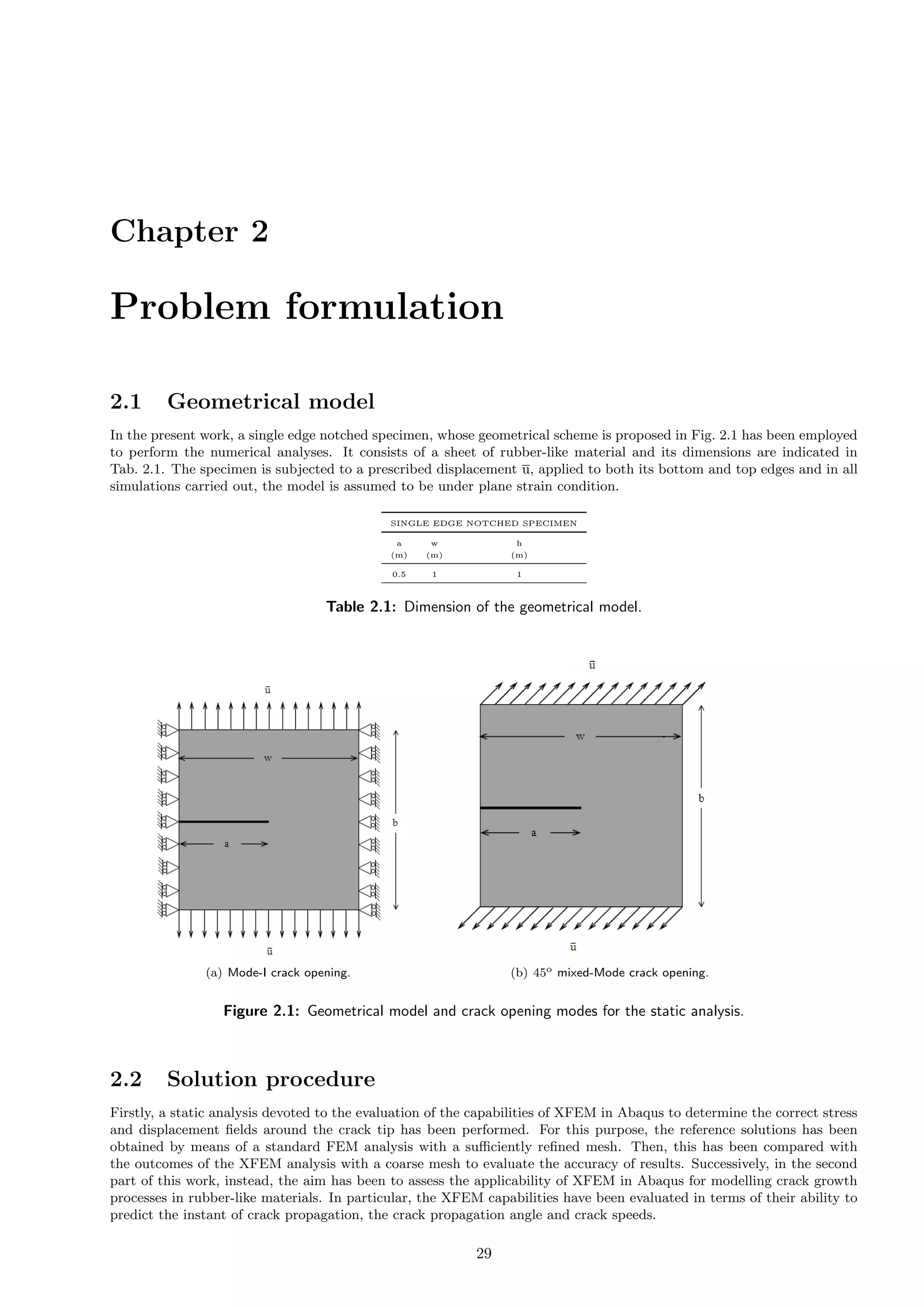
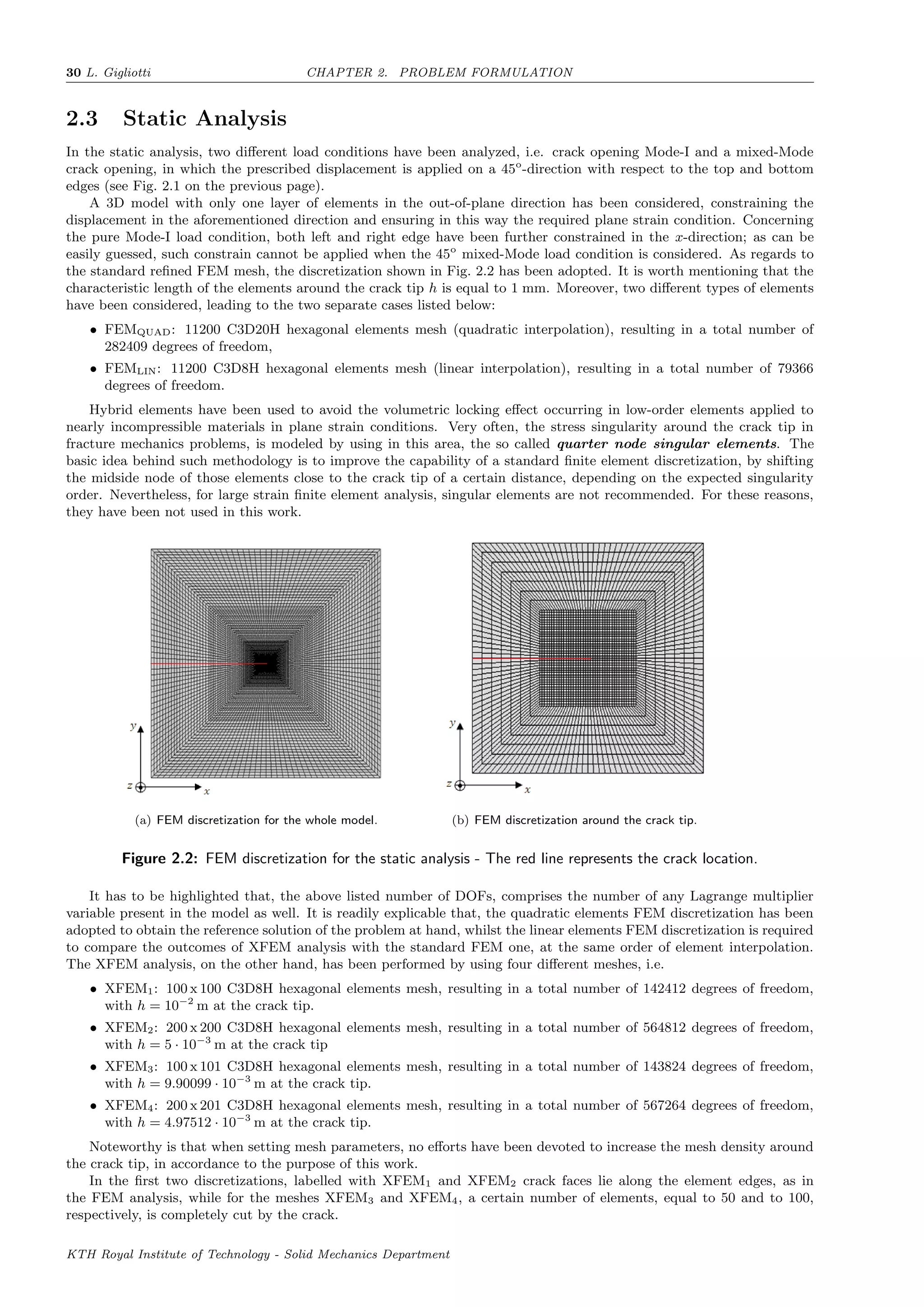
![2.4. DYNAMIC ANALYSIS L. Gigliotti 31
Two different material models have been considered, the Arruda-Boyce model and the Neo-Hookean model. Material
coefficients of both the hyperelastic models may be computed directly in Abaqus/Standard, providing experimental
stress-strain data. Results obtained from three different experimental tests, i.e. uniaxial, equibiaxial and planar test, can
be provided in the Abaqus/Standard environment; material constants will then be calculated by means of a nonlinear
least-square procedure, which minimizes the relative error in stress. Here, experimental uniaxial test data in [12] are
used, and the result of such fitting procedure is depicted in Fig. 2.3.
Figure 2.3: Fitting of uniaxial test data with the Arruda-Boyce and Neo-Hookean model in Abaqus.
2.4 Dynamic Analysis
The dynamic analysis has been carried out, with the same geometric model adopted for the static analysis. The assumed
material model is the Arruda-Boyce, whose parameters are the ones computed in previous section. Two different loading
conditions have been examined in the dynamic analysis; however, in this case, the pure crack opening Mode-I has not
been taken into account, but in addition to the 45o
mixed-Mode, a 30o
mixed-Mode has been analyzed (see Fig. 2.4).
Figure 2.4: 30o
mixed-Mode crack opening.
In order to evaluate the mesh-dependence of the solution, five different discretizations, with decreasing characteristic
element dimension h at the crack tip, have been used, i.e.
• XFEMD1: 2541 C3D8H hexagonal elements mesh, resulting in a total number of 36090 degrees of freedom, with
h = 4.76193 · 10−3
m at the crack tip,
• XFEMD2: 4061 C3D8H hexagonal elements mesh, resulting in a total number of 57610 degrees of freedom, h =
3, 22580 · 10−3
m at the crack tip,
KTH Royal Institute of Technology - Solid Mechanics Department](https://image.slidesharecdn.com/5bffcdff-873e-4f02-b330-da222b639ff8-151115100138-lva1-app6891/75/FULLTEXT01-37-2048.jpg)
![32 L. Gigliotti CHAPTER 2. PROBLEM FORMULATION
• XFEMD3: 5781 C3D8H hexagonal elements mesh, resulting in a total number of 81930 degrees of freedom, h =
2, 43902 · 10−3
m at the crack tip,
• XFEMD4: 7701 C3D8H hexagonal elements mesh, resulting in a total number of 109050 degrees of freedom,
h = 1, 96078 · 10−3
m at the crack tip,
• XFEMD5: 20301 C3D8H hexagonal elements mesh, resulting in a total number of 286650 degrees of freedom,
h = 0, 99009 · 10−3
m at the crack tip.
For graphical reasons, only the first discretization is shown herein in Fig. 2.5; in all other cases, the discretization
scheme is analogous, while the level of refinement at the crack tip is different.
(a) XFEM discretization for the whole model. (b) XFEM discretization around the crack tip.
Figure 2.5: XFEM discretization for the dynamic analysis.
2.5 Damage parameters
In order to observe the expected crack growth phenomenon, damage initiation and propagation criteria had to be defined.
For the prediction of damage initiation in the enriched region, the Abaqus/Standard User’s Manual suggests to use either
the Maximum principal stress damage criterion or the Maximum principal strain damage criterion; in this
work, the first criterion has been adopted. More in detail, it assumes that a crack will nucleate within the body as soon
as the ratio
f =
σmax
σo
max
(2.1)
reaches a value equal to 1. In Eq. 2.1, σo
max represents the maximum allowable principal stress, while the symbol
indicates the Macaulay brackets, used to signify that a purely compressive stress state does not lead to any damage
initiation. Such criteria, define the conditions at which an internal defect will nucleate within the body. However, in
the geometric model adopted, an internal defect is already present. As consequence, under these conditions, the value of
the principal stress does not play a relevant role for the crack propagation analysis. For this reason, its value has been
set equal to 5.57 MPa, corresponding to the highest stress value observed in the stress-strain relation in Fig. 2.3 on the
preceding page. In this way, the remote possibility that another crack had nucleated under the applied loads is avoided.
Much more important is the damage propagation criterion in the case of pre-existing cracks. In such criterion, a scalar
variable D is introduced to represent the overall damage in the material, due to all the active deformation mechanisms.
Its value evolves monotonically from 0 up to 1, where the failure process is completed. For the characterization of the
damage evolution, it is required to define, firstly, the dissipated energy due to failure GC
and afterwards, the damage
variable D evolution, between the initiation of damage and the final complete failure.
The energy-based model for the damage evolution here considered, is based on the calculation of the energy dissipated
during the damage process, named as fracture energy. In case of mixed-Mode loading conditions, several models have
been proposed to calculate the equivalent fracture energy. In the present work, the BK mixed-mode fracture criterion,
presented by Benzeggagh and Kenane in [98] has been adopted. According to such model, particularly suitable when
the critical fracture energies during separation purely along the first and the second shear directions are the same, the
equivalent fracture energy is equal to
GC
equiv = GC
n + GC
s − GC
n
GS
GT
η
(2.2)
where, GS = Gs + Gt, GT = Gn + GS, while η is a material parameter. As clear, the fracture energy (per unit area)
is computed as function of the fracture energy in the normal mode GC
n , in the first shear mode GC
s and in the second
KTH Royal Institute of Technology - Solid Mechanics Department](https://image.slidesharecdn.com/5bffcdff-873e-4f02-b330-da222b639ff8-151115100138-lva1-app6891/75/FULLTEXT01-38-2048.jpg)
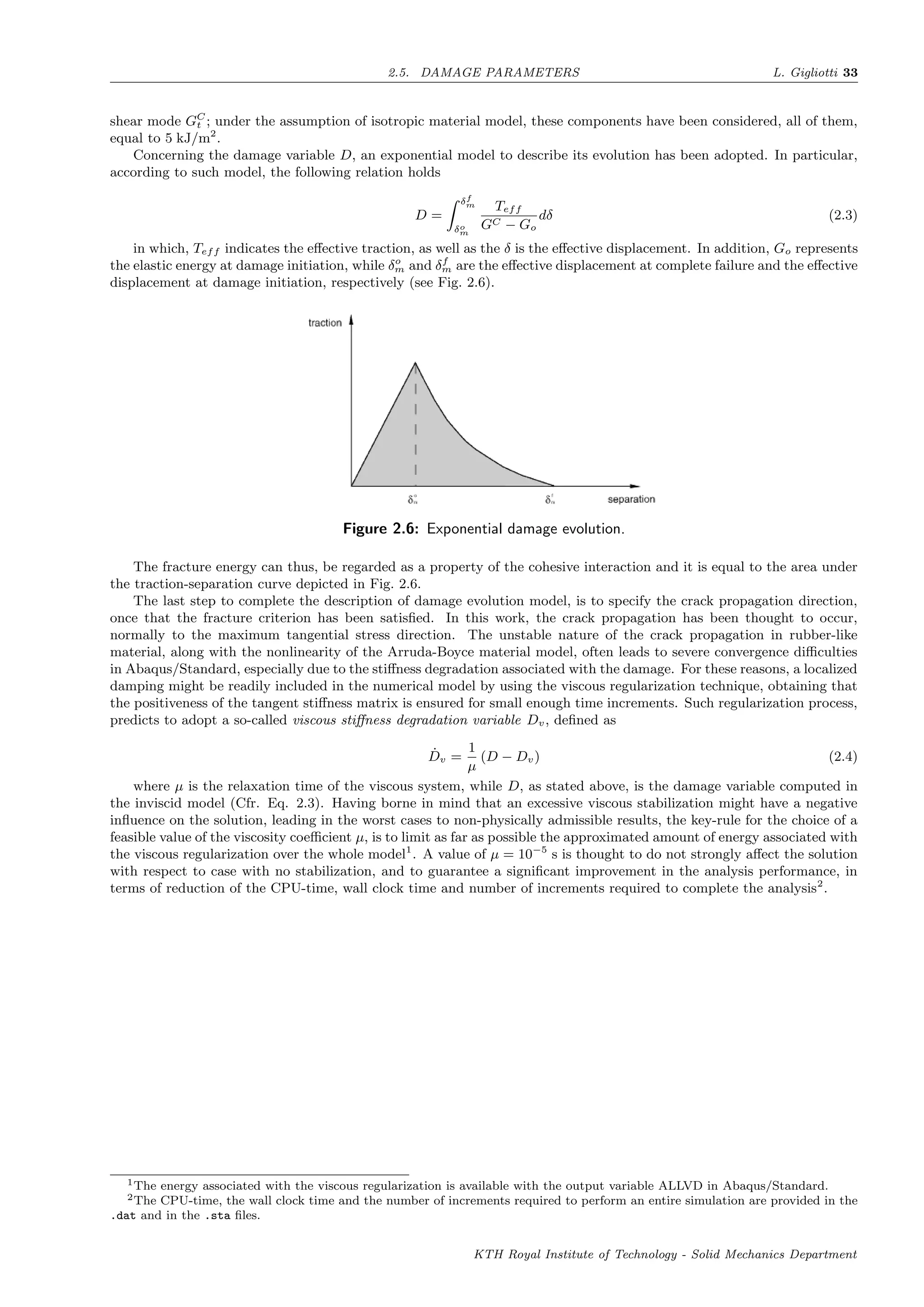

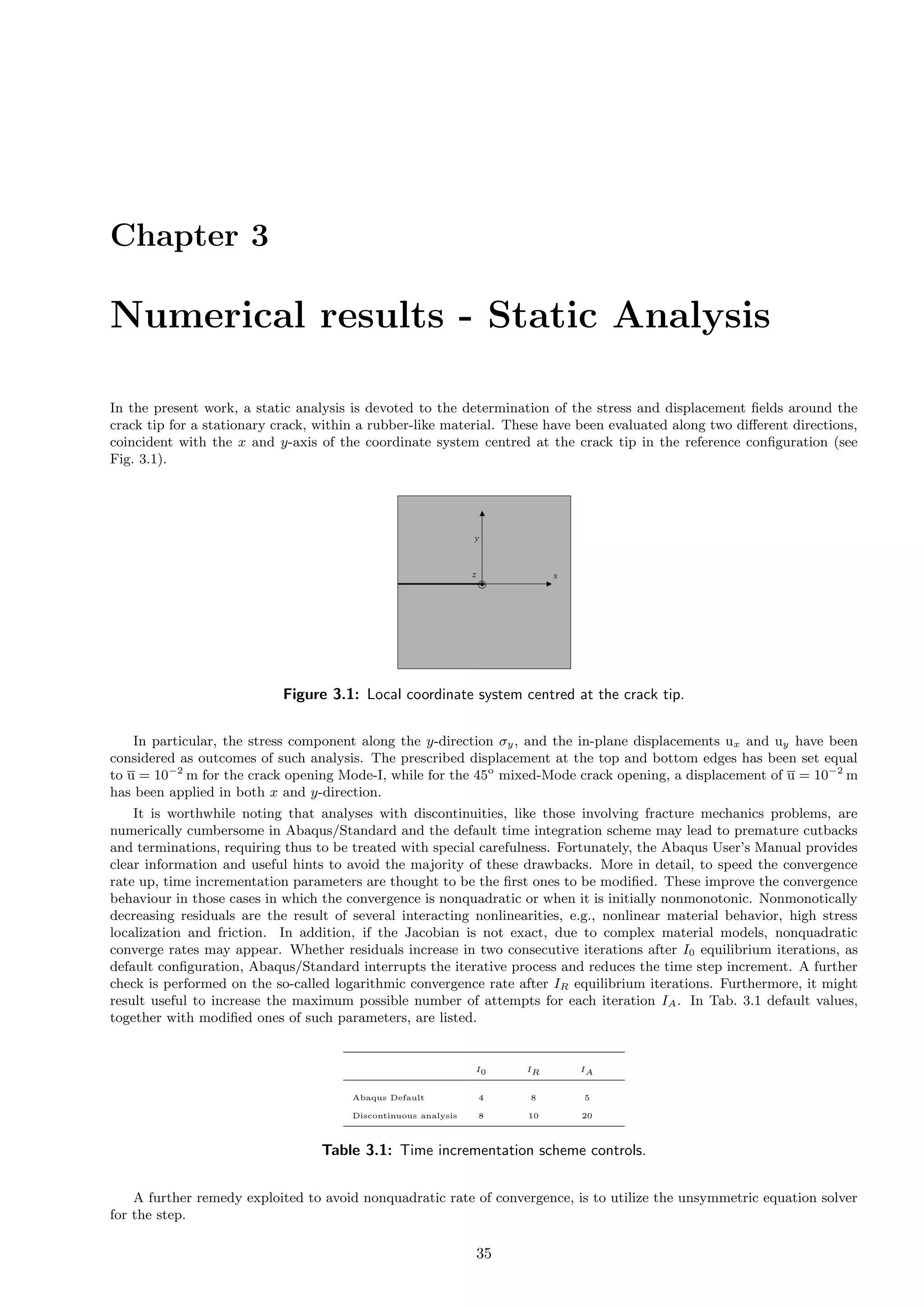
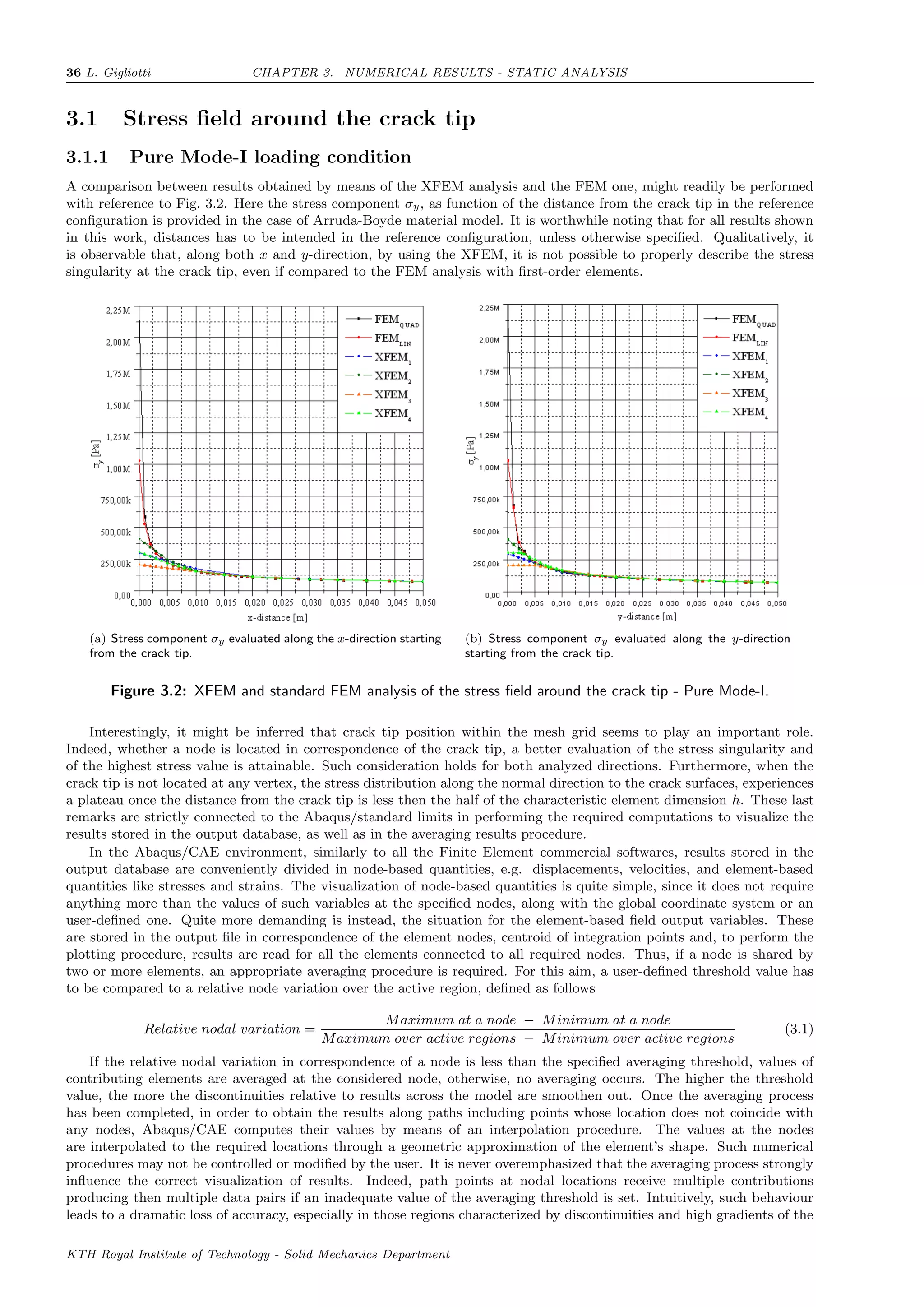
![3.1. STRESS FIELD AROUND THE CRACK TIP L. Gigliotti 37
field outputs. Having the above considerations borne in mind, and given the symmetry of the stress field with respect
to the crack surface, the plateau experienced along the y-direction might be easily justified.
Figure 3.3: Stress values interpolation across the crack surfaces.
Abaqus/CAE linearly interpolates the stress values between the two closest nodes to the crack tip, but since these
values are equal, the interpolation returns a constant stress value. Thus, the addition of a node exactly located at the
crack tip improves such interpolation procedure. Nevertheless, as suggested in [100], for coarse meshes, the condition
number of the system grows if compared to the case where the fracture surfaces do not lie along the edges of the elements.
Lastly, referring to Fig. 3.2 on the facing page, it should be highlighted that, for the direction parallel to crack
surfaces, the XFEM analysis results, strongly deviate from those provided by the FEM analysis at a distance from the
crack tip of 10−2
m. Such distance is halved for the direction normal to the crack tip.
Even if the results discussed above concern the Arruda-Boyce material model, exactly the same considerations are
valid for the case of Neo-Hookean material model.
According to Eq. 1.69, the stress field can be expresses as function of the distance in the reference configuration
from the crack tip r, i.e. σij ∼ r−α
. Based on this, a quantitative analysis of the ability of XFEM to describe the
stress field around the crack tip can be carried out. In fact, the correct evaluation of the exponent in the stress-distance
relation might be used as indicator of quality of the analysis. The closer the numerically evaluated exponent to the
analytical value, i.e. 0.5, the higher is the approximation accuracy1
. Results of such analysis are listed in Tab. 3.2 for
the Arruda-Boyce material model and in Tab. 3.3 for the Neo-Hookean model.
ARRUDA-BOYCE
x-direction y-direction
FEM1 FEM2 XFEM1 XFEM2 XFEM3 XFEM4 FEM1 FEM2 XFEM1 XFEM2 XFEM3 XFEM4
α 0.5 0.446 0.312 0.357 0.239 0.331 0.5 0.451 0.356 0.399 0.27 0.352
R2 (0.9963) (0.9914) (0.842) (0.9089) (0.7876) (0.8843) (0.9964) (0.9735) (0.8903) (0.8081) (0.7351) (0.8462)
Table 3.2: Fitting procedure of the σy stress results for the Arruda-Boyce material model along both
x and y-direction - Pure Mode-I.
NEO-HOOKEAN
x-direction y-direction
FEM1 FEM2 XFEM1 XFEM2 XFEM3 XFEM4 FEM1 FEM2 XFEM1 XFEM2 XFEM3 XFEM4
α 0.5 0.459 0.323 0.338 0.251 0.345 0.499 0.470 0.362 0.403 0.289 0.367
R2 (0.9975) (0.9911) (0.8519) (0.9089) (0.7752) (0.8917) (0.9981) (0.9819) (0.8957) (0.8074) (0.7637) (0.8571)
Table 3.3: Fitting procedure of the σy stress results for the Neo-Hookean material model along both
x and y-direction - Pure Mode-I.
1For the incompressible plane strain case, theoretical results can be found in [101].
KTH Royal Institute of Technology - Solid Mechanics Department](https://image.slidesharecdn.com/5bffcdff-873e-4f02-b330-da222b639ff8-151115100138-lva1-app6891/75/FULLTEXT01-43-2048.jpg)
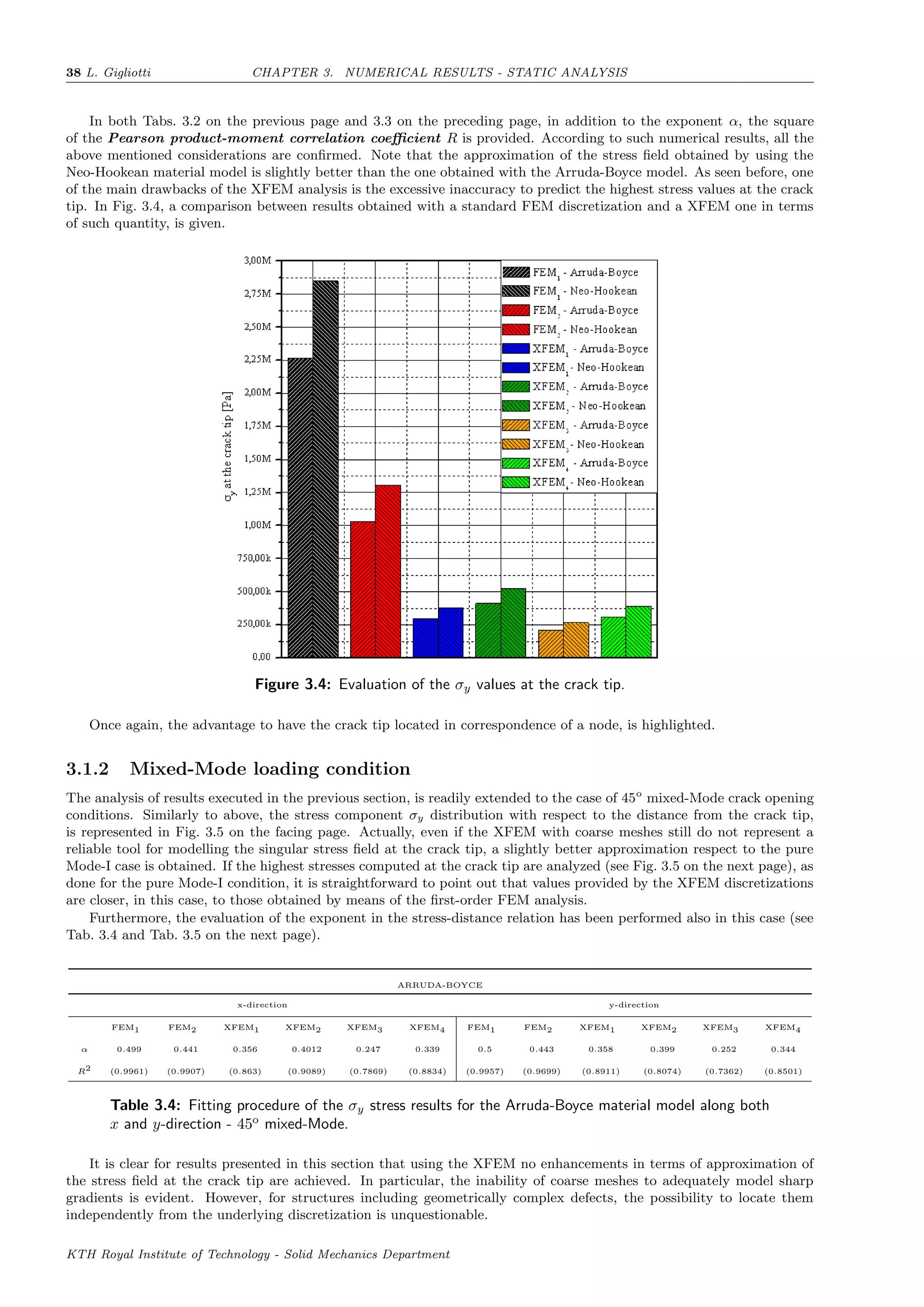
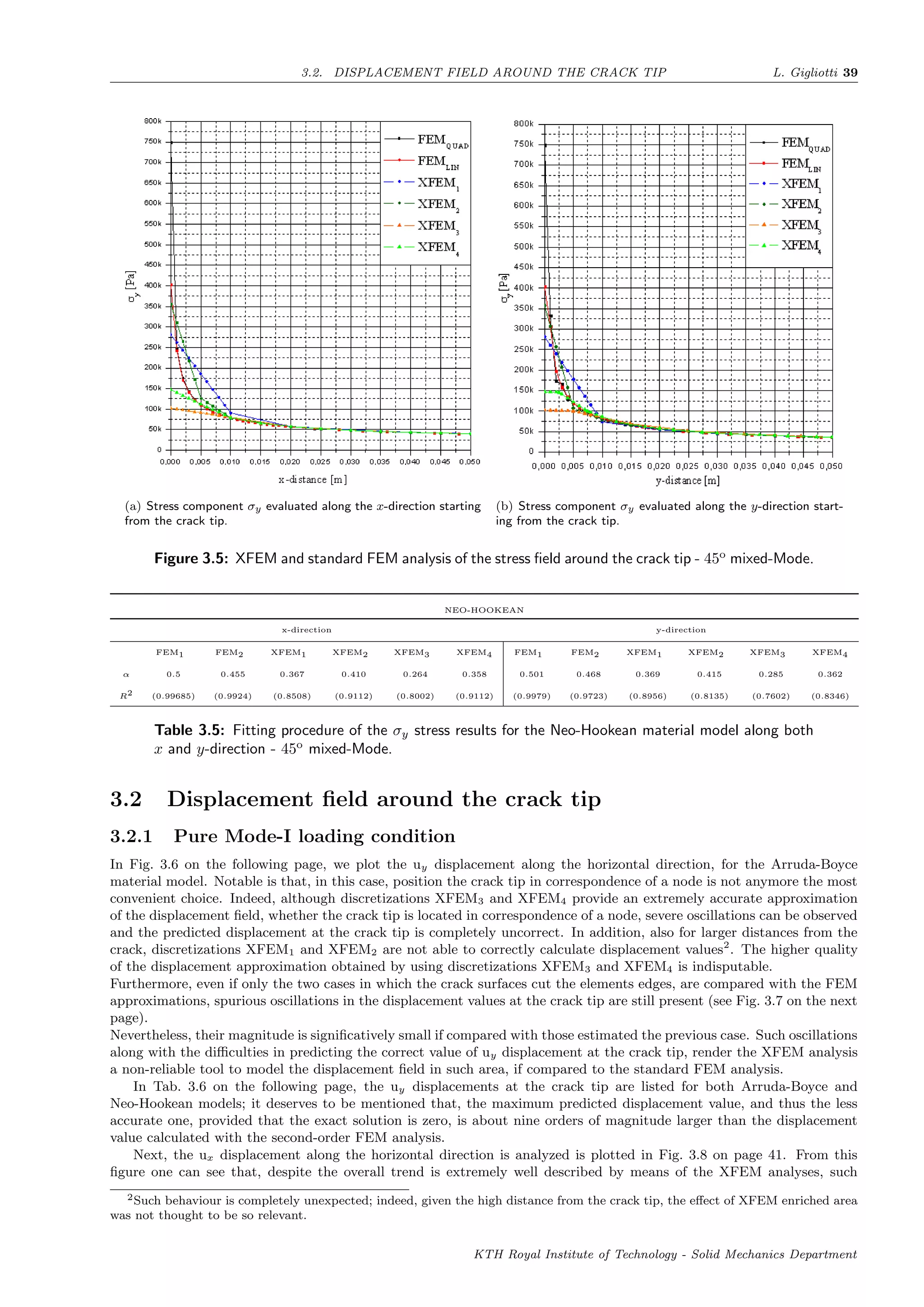
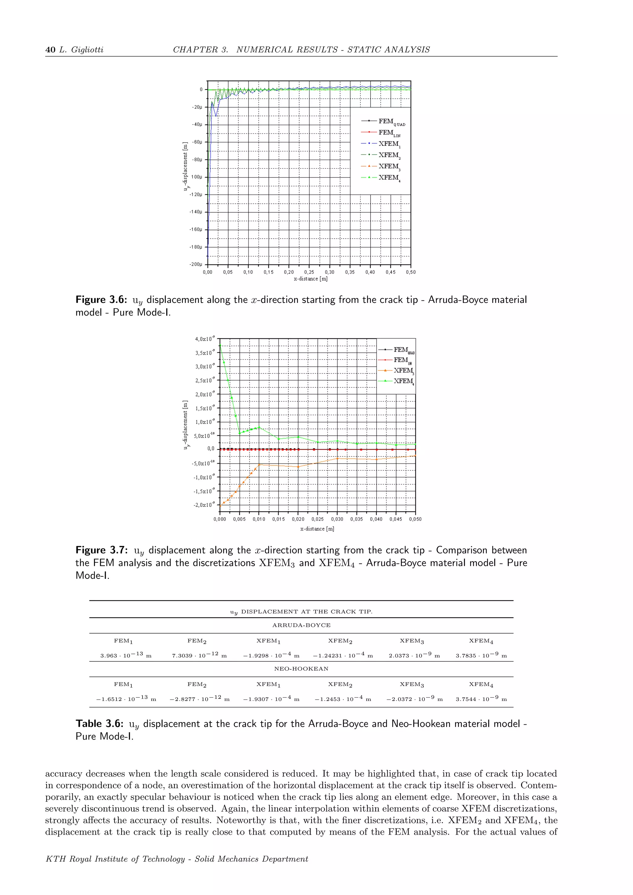
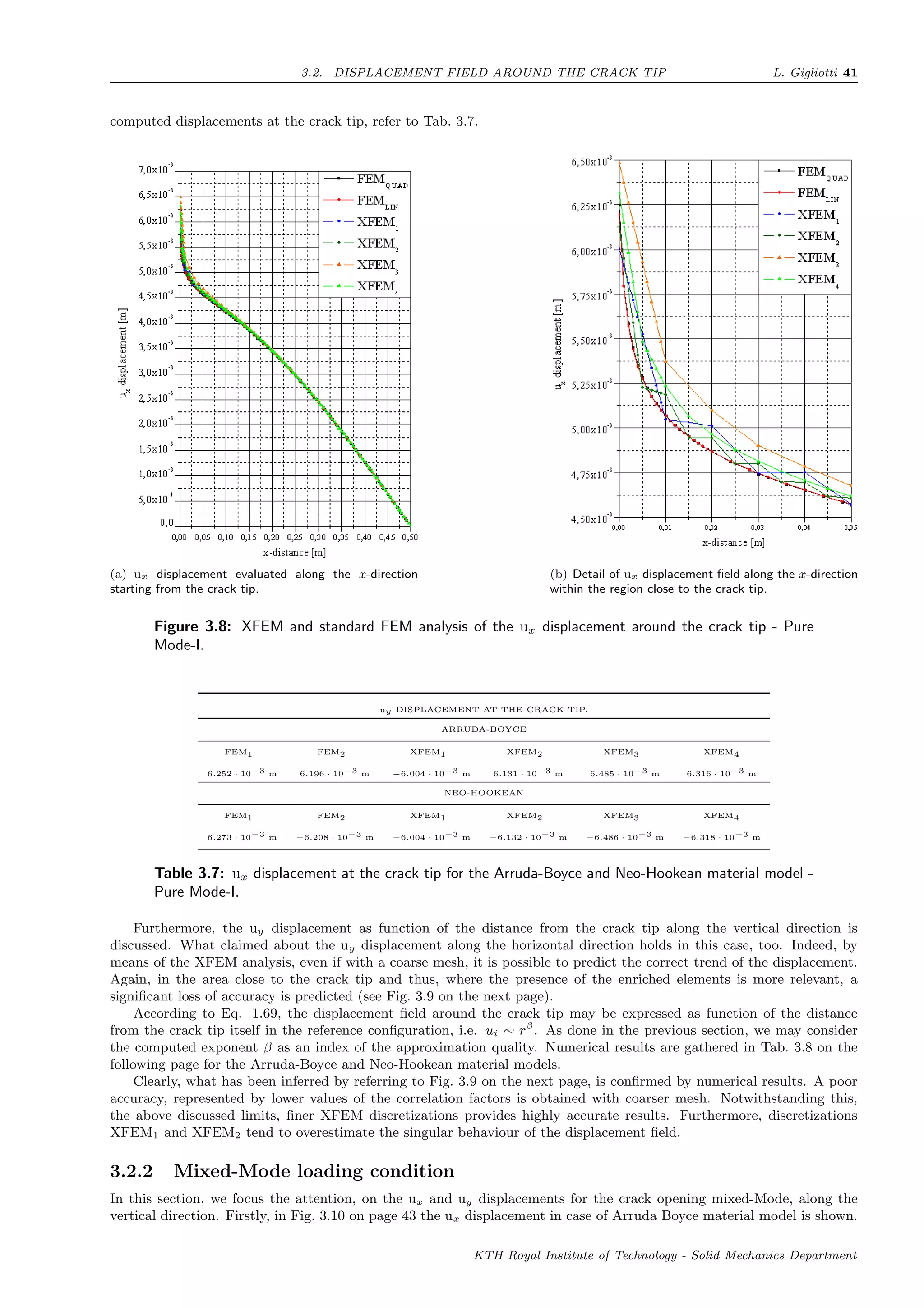
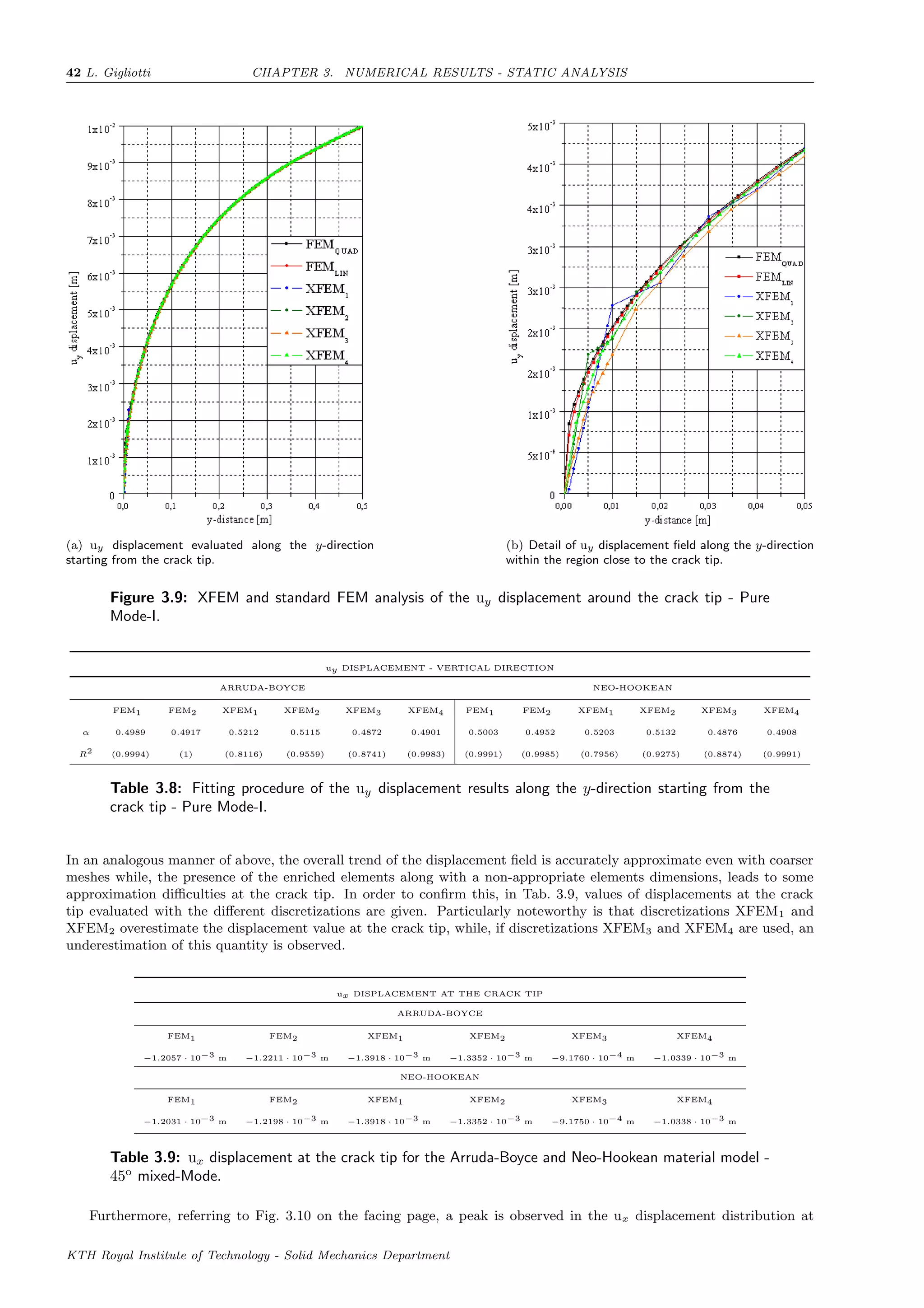
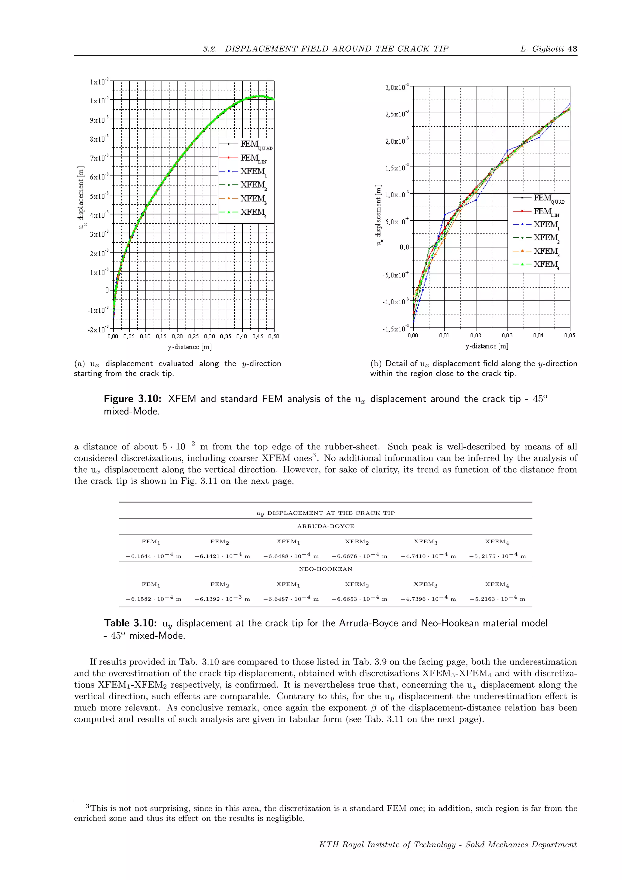
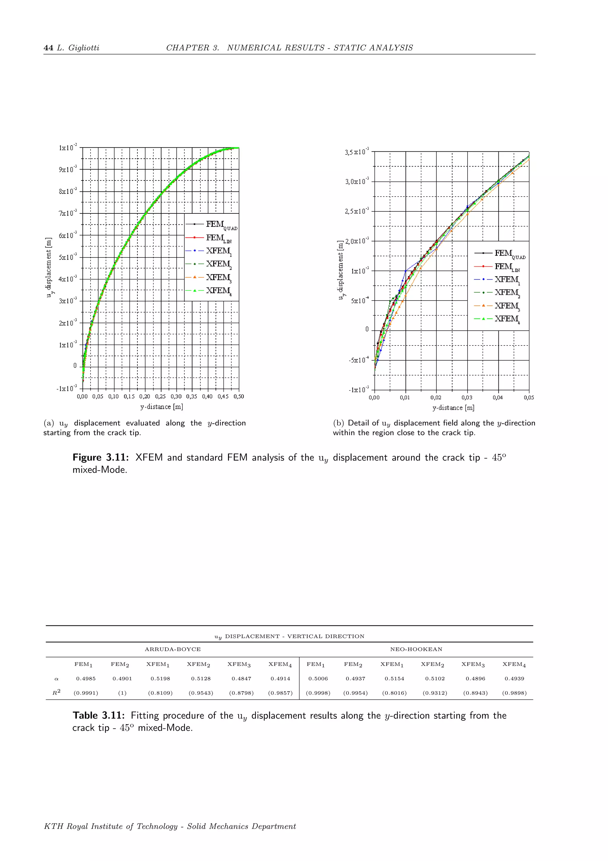
![Chapter 4
Numerical results - Dynamic Analysis
In this second part of the present work, the capabilities of the XFEM in Abaqus have been investigated. The analysis of
the crack propagation phenomenon in rubber-like materials, by using the XFEM technique, has proved to be an arduous
task. This is thought to be mainly due, to the still poor implementation of the XFEM capabilities, along with the
well-established numerical difficulties encountered when fracture mechanics problems are analyzed by using numerical
methods. In particular, tremendous convergence difficulties have been faced and still unsatisfactory results in performing
numerical simulations of the crack growth process have been obtained. Only few elements can be cracked before the
simulation is aborted and there seems to be no correlation with the crack length; in other words, the highest number of
cracked elements does not depend on the level of refinement at the crack tip.
Notwithstanding these problems, three fundamental aspects of the crack propagation phenomenon have been inves-
tigated, i.e. the instant at which, under the applied boundary conditions, the pre-existing crack starts to propagate, the
crack propagation angle and the crack propagation speed. For this aim, the above discussed discretizations have been
employed (Cfr. Sec. 2.4). The choice to use discretizations in which the crack is not aligned with the elements edges, has
been somehow forced. Indeed, even with extreme modifications (sometimes almost non-realistic) of the time integration
scheme and of convergence parameters, it has been impossible to observe any crack growth in case of crack surfaces lying
along elements edges. Likely, this stems from the presence of the node in correspondence of the crack tip and thus, from
the resulting poorly conditioned problem (Cfr. Sec. 3.1.1). Furthermore, both the effects of the applied displacement
and of the applied displacement rate have been taken into account.
4.1 Convergence criteria for nonlinear problems
As first attempt, the crack propagation phenomenon has been analyzed by means of a Static stress/displacement analysis.
However, likely due to the unstable nature of the crack propagation process, by utilizing such typology of analysis it has
been not possible to observe any crack propagation and furthermore, no simulations have been successfully completed.
The Newton-Raphson method employed in Abaqus/Standard, when unstable processes are considered, often shows
severe problems in reaching the convergence. However, these shortcomings are partially enhanced in dynamic problems
by the introduction of the mass matrix M, which is an additional positive term to the Jacobian. In such way, the Jacobian
is thus slightly more positive and inertia effects help to regularize unstable behaviours1
. Based on these considerations,
an implicit dynamic analysis has been performed2
.
Interestingly, what has been regarded as a limit, i.e. the possibility to use only linear elements, in this case is
transformed into an advantage. Indeed, in large-deformation problems higher-order elements are affected by a rapid loss
of accuracy, since the Jacobian determinant can be easily become negative at quadrature points, causing the abortion
of calculations and high local inaccuracies. Thus, the implementation of higher-order XFEM could not lead to any
significant enhancement.
Noteworthy is that, for all simulations performed, the maximum time step increment has been set equal to 0.1% of
the whole simulation time3
. By starting from zero, the applied displacement is linearly ramped over the step, until the
prescribed value at the bottom ant top edge has not been reached.
In Abaqus/Standard, dynamic problems might be classified within three categories, i.e. transient fidelity applications,
moderate dissipation applications and quasi-static applications. The Hilbert-Hughes-Taylor time integration method
[102] is used for transient fidelity and moderate dissipation applications while the backward Euler operator is employed
if the application is identified as quasi-static. Concerning this latter, it should be stressed that its application in Abaqus,
requires a particular carefulness, because it automatically induces a 5% numerical damping and this value cannot be
modified by the user. Especially for this last reason, the Hilbert-Hughes-Taylor method has been used and its coefficients
have been tuned to attain a moderate numerical damping, which should help convergence and at the same time, not
1The density of rubber-like material has been set equal to 1000 kg/m3.
2The principal advantage of this method is that it is unconditionally stable and thus no limitations exist on the size of time
increment used for the integration.
3Comprehensive discussion on the correct choice of the maximum time step increment is provided on the Abaqus User’s Manual
(Cfr. Sec. 7.1.1).
45](https://image.slidesharecdn.com/5bffcdff-873e-4f02-b330-da222b639ff8-151115100138-lva1-app6891/75/FULLTEXT01-51-2048.jpg)
![46 L. Gigliotti CHAPTER 4. NUMERICAL RESULTS - DYNAMIC ANALYSIS
overly affect the physical formulation of the problem at hand 4
. The HHT method provides for the definition of three
different parameters, α, β and γ. In order to let the method satisfy the stability and order properties [103], these
parameters are not independent of each other, but the following relationships hold
γ = 1−2α
2
; β = (1−α)2
4
(4.1)
Consequently, it is sufficient to modify only the parameter α to obtain different levels of numerical damping. The
choice of α equal to 0, leads to the simple trapezoidal method and therefore, no numerical damping is introduced. On
the other hand, the maximum numerical damping, i.e. 6%, is obtained for α = −1/3. For a comprehensive discussion on
the appropriate values of HHT-method parameters, refer to [104]. The values of such coefficients, utilized in this work
are listed in Tab. 4.1.
HILBERT-HUGHES-TAYLOR METHOD COEFFICIENTS
β γ α
0.3025 0.6 −0.1
Table 4.1: Modified parameters for the Hilbert-Hughes-Taylor operator.
In addition to the introduction of numerical damping, the time implementation scheme has been adjusted analogously
to the static analysis discussed in the previous chapter. Furthermore, the Criterion for residual forces for nonlinear
problems and the Criterion for displacement correction in nonlinear problems have been modified. In order to
explain these latter modifications, let us denote with α the characteristic field related to a particular problem, e.g. the
displacement field in stress analyses. The parameters commonly used to determine whether an increment has converged
or not, are the following ones:
rα
max , the largest residual for the equilibrium equation of the field α;
∆uα
max , the maximum variation of the nodal variable during the increment;
cα
max , the largest correction executed during the current Newton iteration on any variable of type α;
ej
, the greatest error in the particular j-constraint type, e.g. volumetric strain compatibility in problems involving
hybrid elements;
qα
(t) , the magnitude of the conjugate flux to the field α, e.g. force flux for the displacement field, at any time t; it
represents a spatial average flux over the entire domain, and it is defined a follows
qα
(t)
def
=
E
e=1
Ne
ne=1
Nα
ne
i=1 |q|α
i,ne
+ i=1
Nα
ef
|q|α,ef
i
E
e=1
Ne
ne=1 Nα
ne
+ Nα
ef
(4.2)
where E is number of elements of the whole model, Ne is the number of nodes of the element e, Nα
ne
indicates the
number of α-DOFs at the node ne of the element e, |q|α
i,ne
represents the magnitude of the flux that the element
e applies at its i-th α-DOF at its ne-th node at the specified time t, Nα
ef denotes the number of external fluxes for
the α-field and lastly, |q|α,ef
i is the amplitude of the i-th external flux for the α-field;
qα
(t) , the overall time-averaged value of the conjugate flux to the field α; such averaging is performed over the whole
step, i.e.
qα
(t)
def
=
1
Nt
Nt
i=1
qα
(ti) (4.3)
in which Nt indicates the total number of increments made hitherto in the step, including the current one as well.
For many practical applications, the following condition on the error in the residuals is introduced
rα
max ≤ Rα
nqα
(4.4)
Once the Eq. 4.4 is satisfied, the solution is accepted as converged if the largest correction to the solution cα
max is
smaller than the greatest variation in the solution variable ∆uα
max, i.e.
cα
max ≤ Cα
n ∆uα
max. (4.5)
Coefficients Rα
n and Cα
n control the criterion for residual forces for nonlinear problems and the criterion for displace-
ment correction in nonlinear problems, respectively, provided that the considered displacement field α, is the displacement
one. In Tab. 4.2 on the next page, both default and updated values of such parameters are given.
4The HHT method is an extension of the Newmark β method.
KTH Royal Institute of Technology - Solid Mechanics Department](https://image.slidesharecdn.com/5bffcdff-873e-4f02-b330-da222b639ff8-151115100138-lva1-app6891/75/FULLTEXT01-52-2048.jpg)
![4.2. CRACK PROPAGATION INSTANT L. Gigliotti 47
Rα
n Cα
n
Abaqus Default 5 · 10−3 10−2
User controls 10−2 2 · 10−2
Table 4.2: Criteria for nonlinear problems controls.
4.1.1 Line search algorithm
Apart from modifying the aforementioned coefficients, in order to ameliorate the convergence and increase the robustness
of Newton-Raphson method, the line search algorithm has been included in the analysis. The main idea behind such
algorithm is that, although the direction predicted by the ordinary Newton-Raphson method ∆d often is a good one
towards the correct solution, the step size ∆d frequently is not the optimal one.
In the line search algorithm, the minimization of a measure of residuals, along the line d = dold +λ∆d, is sought. The
parameter λ defines the position along the line d, while dold is the last iterate. In nonlinear problems characterized by
sharp discontinuities in the solution, the line search method represents a powerful tool to reduce the number of iterations
and cutbacks, resulting thus in a reduction of computational cost.
An aggressive line searching has been utilized in this work. In particular, the maximum number of line search
iterations allowed, Nls
, is 10, while the accuracy in the line scale factor ηls
employed, has been considered equal to 10−2
.
4.2 Crack propagation instant
In this section, the instant at which the pre-existing crack starts to propagate within the structure is studied by using
the XFEM technique. As previously stated, in Abaqus/Standard a crack can propagate only by completely cutting each
element that it goes through. Based on this, the crack propagation instant tcrack is defined as the instant at which
the first element is cut by the advancing crack. Such value has been calculated with a precision up to a thousandth of
second5
.
First of all, an iterative procedure has been devoted to identify the value of displacement which causes the crack to
propagate only within a single element. The instant of time at which this occurs is referred to as a reference crack
propagation instant tcrack. Such procedure has been performed by utilizing the discretization XFEMD5. Furthermore,
it has been observed that, whether the crack crosses just one element, the simulations are able to terminate reaching the
convergence. Provided this, the calculated value of the reference crack propagation instant can be correctly evaluated.
Difficulties are encountered when the applied displacement rises and when coarser mesh at the crack tip are employed.
Concerning the applied displacement, five different values have been considered, starting from 3 · 10−2
m up to a value
of 5 · 10−2
m, while keeping the velocity at which it is applied, at the constant value of v = 10−3
m/s. The fulfillment of
quasi-static conditions, has been kept under control by verifying the value of the total kinematic energy of the model6
.
In order to assess the influence of the applied displacement as well as of the element size at the crack tip, on the correct
determination of the parameter at hand, the percent error, defined as follows, has been exploited
Error [%] =
tcrack − tcrack
tcrack
· 100 (4.6)
Such quantity is shown in Fig. 4.1 on the following page as function of the applied displacement u and for different
elements sizes h at the crack tip.
It can be easily seen that, in this case, the effect of the applied displacement is almost inexistent since the percentage
error remains constant with the applied displacement.
As expected, it is noted that the element size, on the contrary, strongly affects the results. Such statement is further
confirmed referring to Fig. 4.2 on the next page. Here, the percentage of error as function of the element size at the
crack tip h is depicted for both mixed-Mode load conditions analyzed. An almost linear trend can be easily noticed,
although a slight deviation is observed in correspondence of intermediate values, i.e. for h ≈ 2 · 10−2
m. In both cases,
a portion of the graph has been shown with an higher level of detail, in order to visualize the, albeit slight, influence of
the applied displacement.
So far, we have considered a constant applied displacement velocity of 10−3
m/s. We may now analyze the effect of
such quantity on the evaluation of the crack propagation instant. In Fig. 4.3 on page 49 the evolution of the percentage
error defined above, is presented. In all cases, the applied displacement rate v is, on purpose, higher than v. Compare
such figure with the analogous one regarding the influence of the applied displacement. Note that although the results are
almost identical, a slight dependence on the applied displacement rate v is detected. Especially for coarser discretizations
at the crack tip, the higher the applied displacement rate v, the higher the percentage error.
5The small size of the time step increments during the crack propagation process allow us to achieve such high level of accuracy.
6Furthermore, information indicating whether the quasi-static conditions are satisfied or not, are provided in the .dat
Abaqus/CAE file.
KTH Royal Institute of Technology - Solid Mechanics Department](https://image.slidesharecdn.com/5bffcdff-873e-4f02-b330-da222b639ff8-151115100138-lva1-app6891/75/FULLTEXT01-53-2048.jpg)
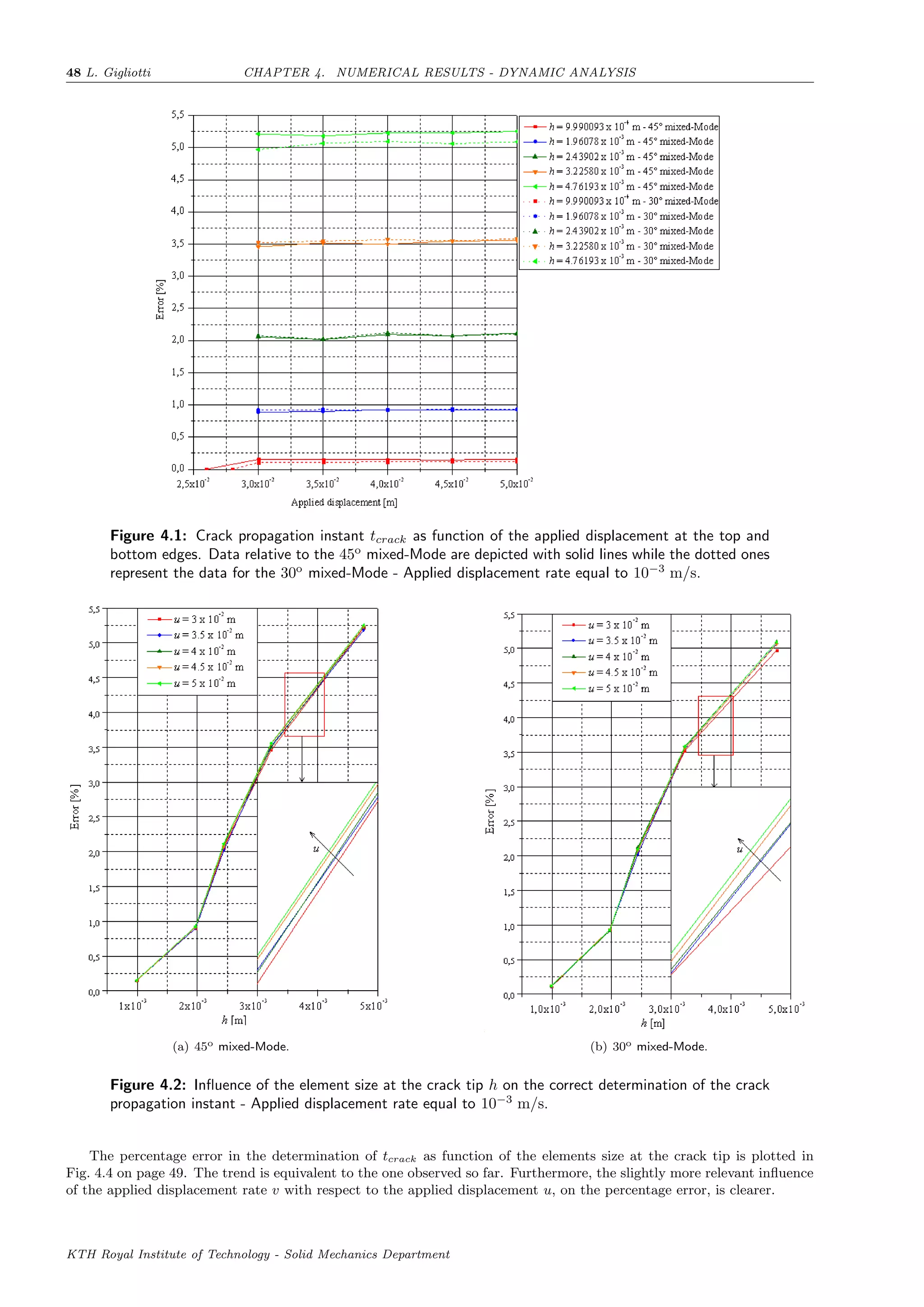
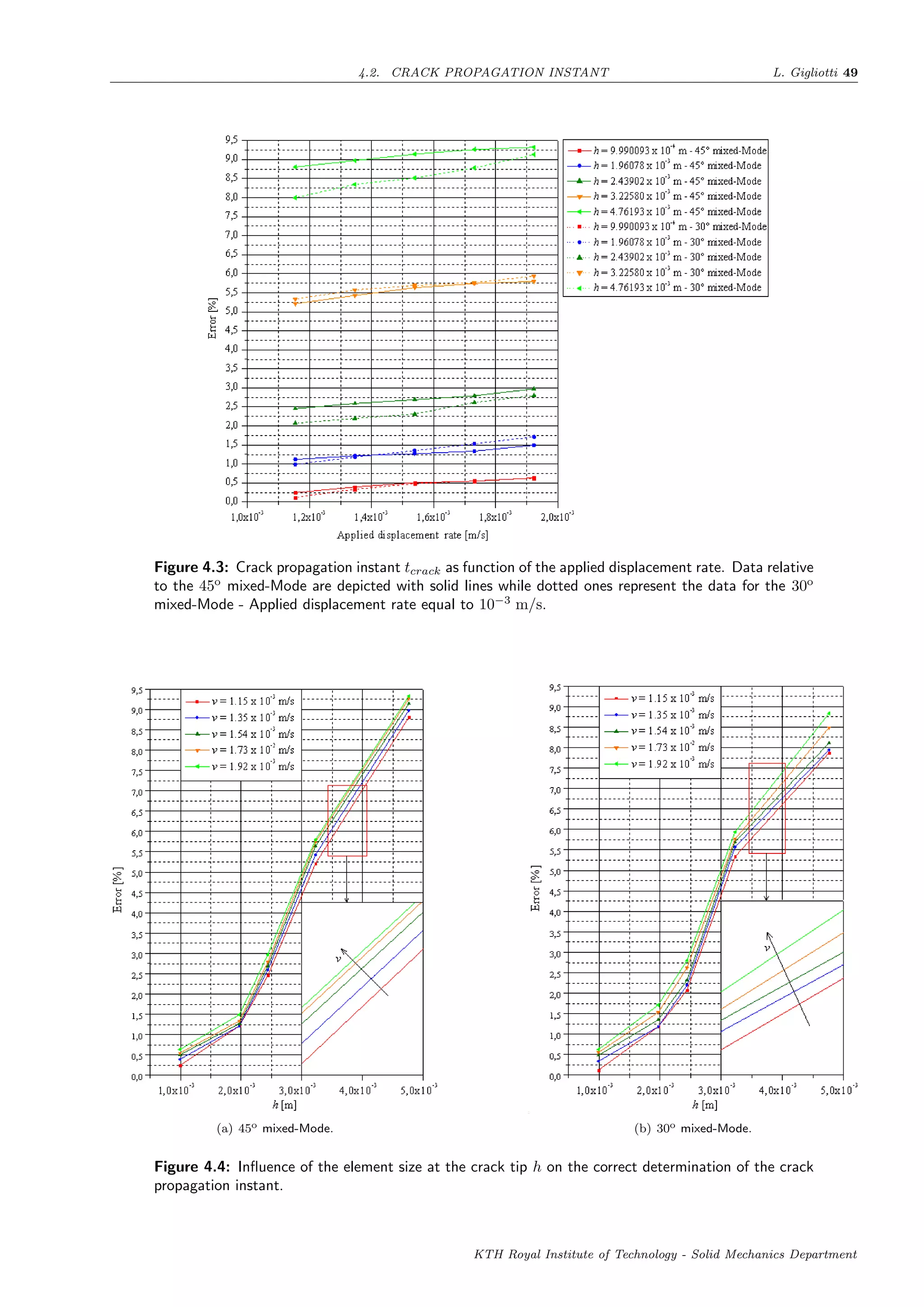
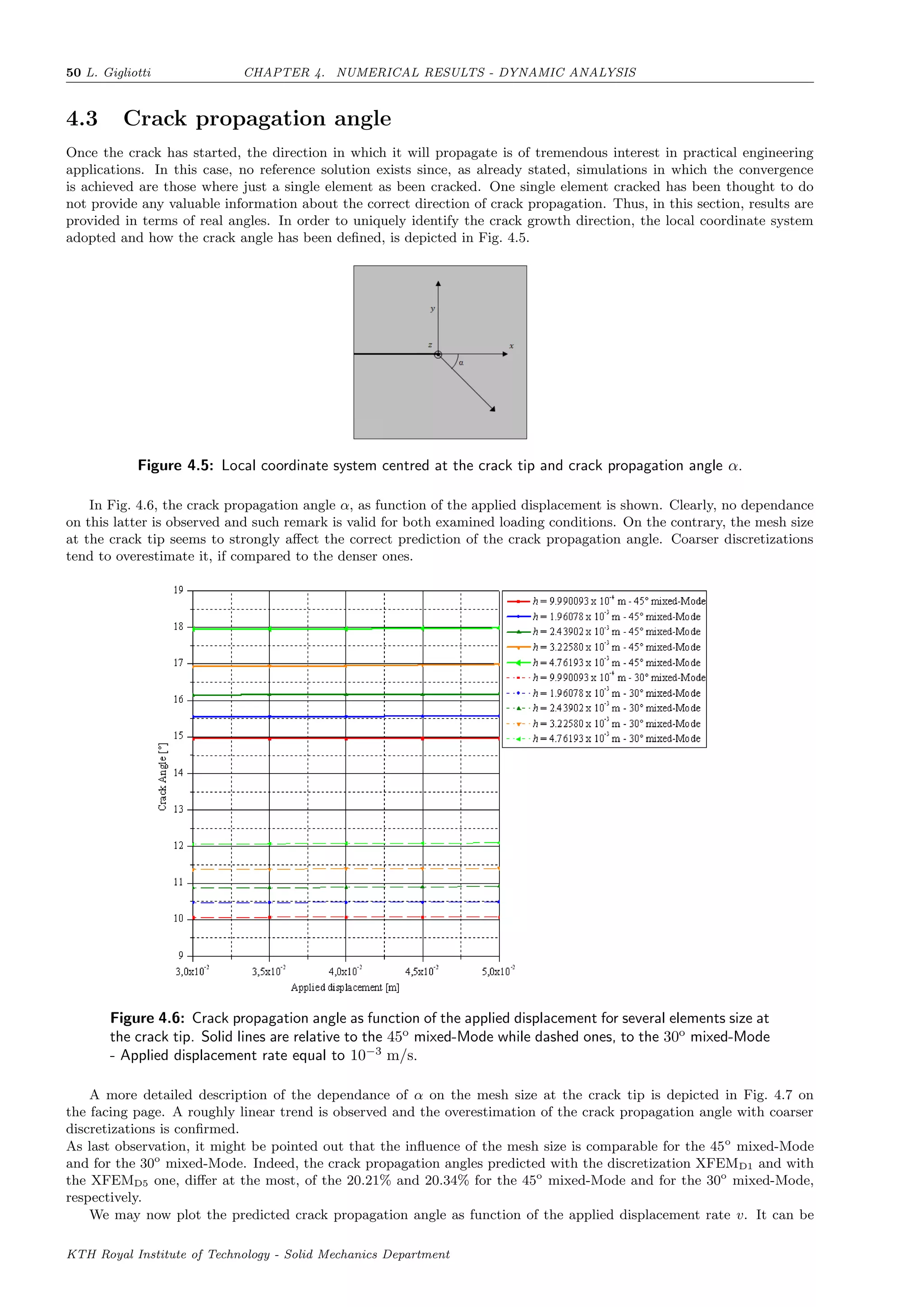
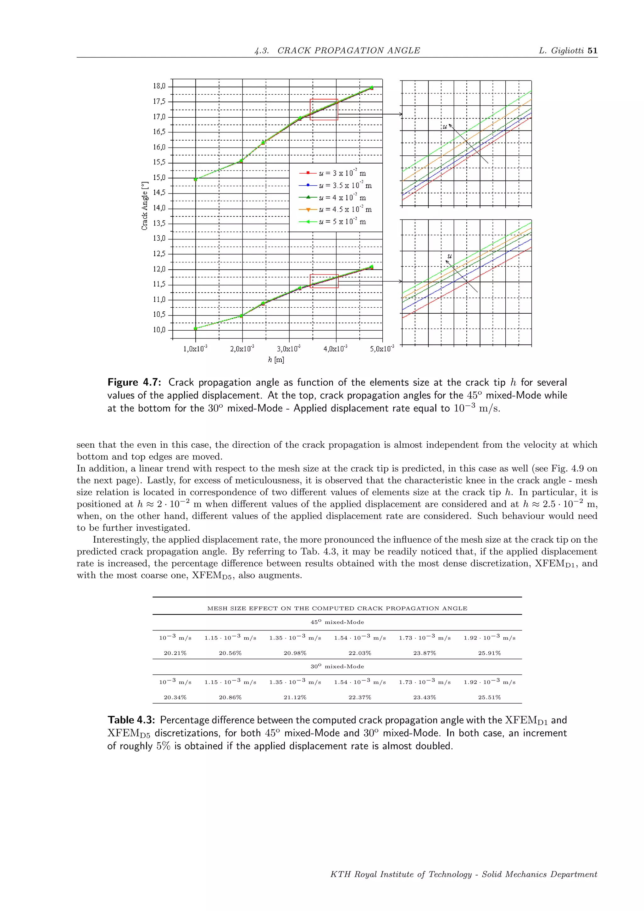
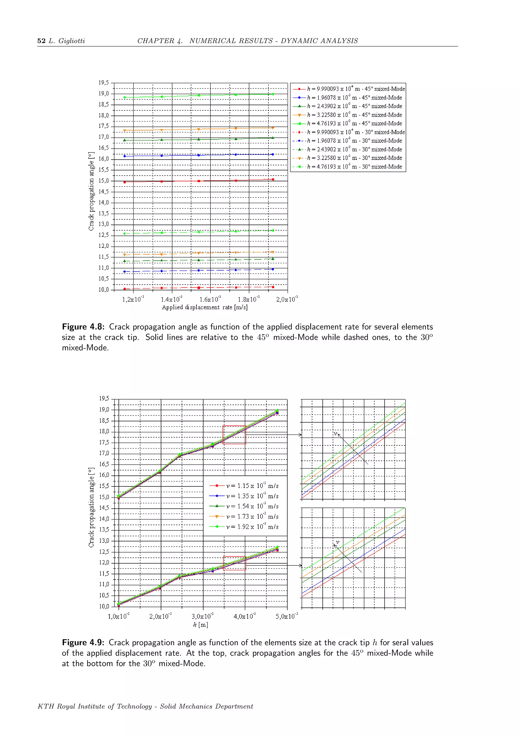
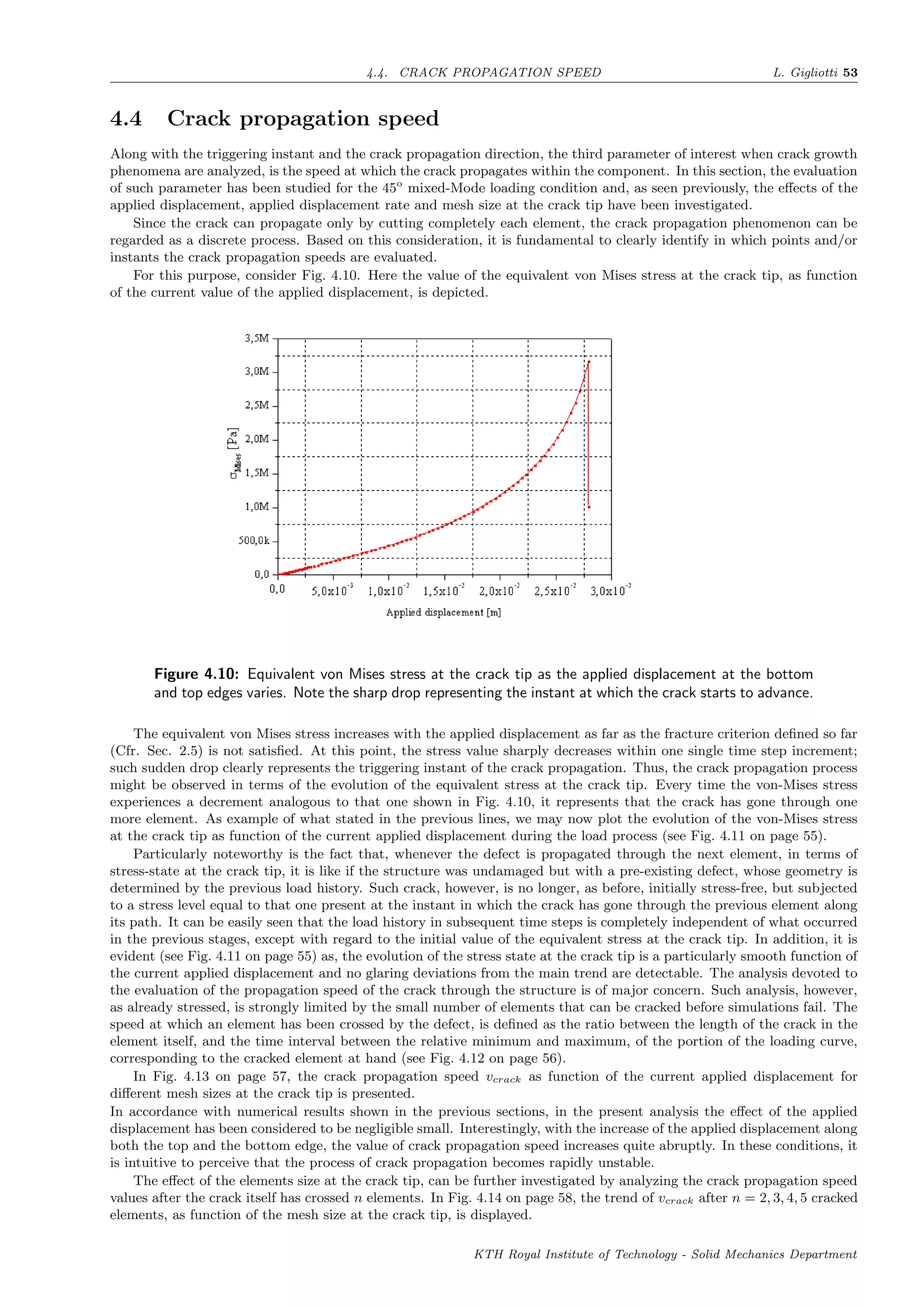
![54 L. Gigliotti CHAPTER 4. NUMERICAL RESULTS - DYNAMIC ANALYSIS
One can clearly deduce that in all cases analyzed, coarser meshes tend to underestimate the value of the crack propagation
speed. This effect is much more pronounced as the lower vcrack itself, i.e. when the crack is starting to propagate. The
percentage variation, between the values calculated by using the most dense mesh XFEMD5 or the most coarse one
XFEMD1, is given in Tab. 4.4.
MESH SIZE INFLUENCE ON vcrack
n = 2 n = 3 n = 4 n = 5
48.56% 40.54% 32.17% 19.02%
Table 4.4: Influence of the mesh size on vcrack. The percentage differences listed are relative to the
variation of the crack propagation speeds predicted with discretizations XFEMD1 and XFEMD5.
Observe that the crack propagation speed has not exceeded in any case the velocity of 50 m/s. This latter is
considered a threshold value above which, the effects of inertia can no longer be neglected [105]. As conclusion of
the present work, the influence of the applied displacement rate on the estimated crack propagation speed is studied.
Following the same procedure adopted so far, consider the evolution of the equivalent von-Mises stress at the crack tip
as function of the applied current displacement (see Fig. 4.15 on page 59) for a value of the applied displacement rate
equal to 1.92 · 10−3
m/s and for five different element sizes at the crack tip7
. Compare this result with that one shown
in Fig. 4.11 on the facing page. In this case, one can observe how the trend is not completely uniform, showing on the
contrary, a highly irregular behaviour.
Therefore, increasing the applied displacement rate, an additional source of instability of the model is introduced. Likely,
this is due to the fact that, if the specimen is loaded with a higher velocity, the inertia effects ca no longer be neglected.
In order to better characterize such unstable behaviour, it is sufficient to evaluate the kinetic energy of the whole
model and compare it to its total internal energy. To fulfil the quasi-static conditions, the kinetic energy should remain
below the 5% of the internal energy during the majority of the analysis. Such condition, as already stated, is completely
satisfied for an applied displacement rate equal to 10−3
m/s. However, when higher values are considered, even if this
condition continues to be met, the threshold value of 5% becomes progressively closer during some steps, and such
situation is thought to lead to a further model instability.
Nevertheless, in Fig. 4.16 on page 60 the crack propagation speed as function of the current applied displacement
and for five different element sizes at the crack tip, is presented. It is confirmed that, as the displacement at the bottom
and top edge increases, the vcrack rises dramatically up to values higher then those observed in the previous case, for an
applied displacement rate of 10−3
m/s. These higher values are obviously ascribable to the increased applied displacement
rate. Also in this case, the coarser the mesh the lower the computed crack propagation speed.
In conclusion, we present the evolution of the crack propagation speed as function of the applied displacement rate.
This is shown in Fig. 4.17 on page 61 for four different time steps, namely, after that 2,3,4 and 5 elements have been
completely cracked. As expected, increasing the applied displacement rate, we observe a growth in terms of crack
propagation speed. Moreover, the higher the number of cracked elements and therefore, the predicted propagation
speed, the more pronounced this effect. It seems to be not possible to extrapolate a common trend in all four depicted
cases, however, a nearly parabolic relationship between the applied displacement rate and the crack propagation speed,
is thought to be the most reasonable.
In confirmation of what stated above, regarding the no longer negligible inertia effects, note that for applied displace-
ment rate values equal to 1.73 · 10−3
m/s and 1.92 · 10−3
m/s, the threshold value of 50 m/s for the crack propagation
speed has been exceeded, i.e. 57.691 m/s and 66.043 m/s respectively. In case of applied displacement rate equal to
1.54 · 10−3
m/s, a very close value, equal to 48.021 m/s, is obtained.
7Exactly as above, only a particular example has been shown for graphical reasons.
KTH Royal Institute of Technology - Solid Mechanics Department](https://image.slidesharecdn.com/5bffcdff-873e-4f02-b330-da222b639ff8-151115100138-lva1-app6891/75/FULLTEXT01-60-2048.jpg)
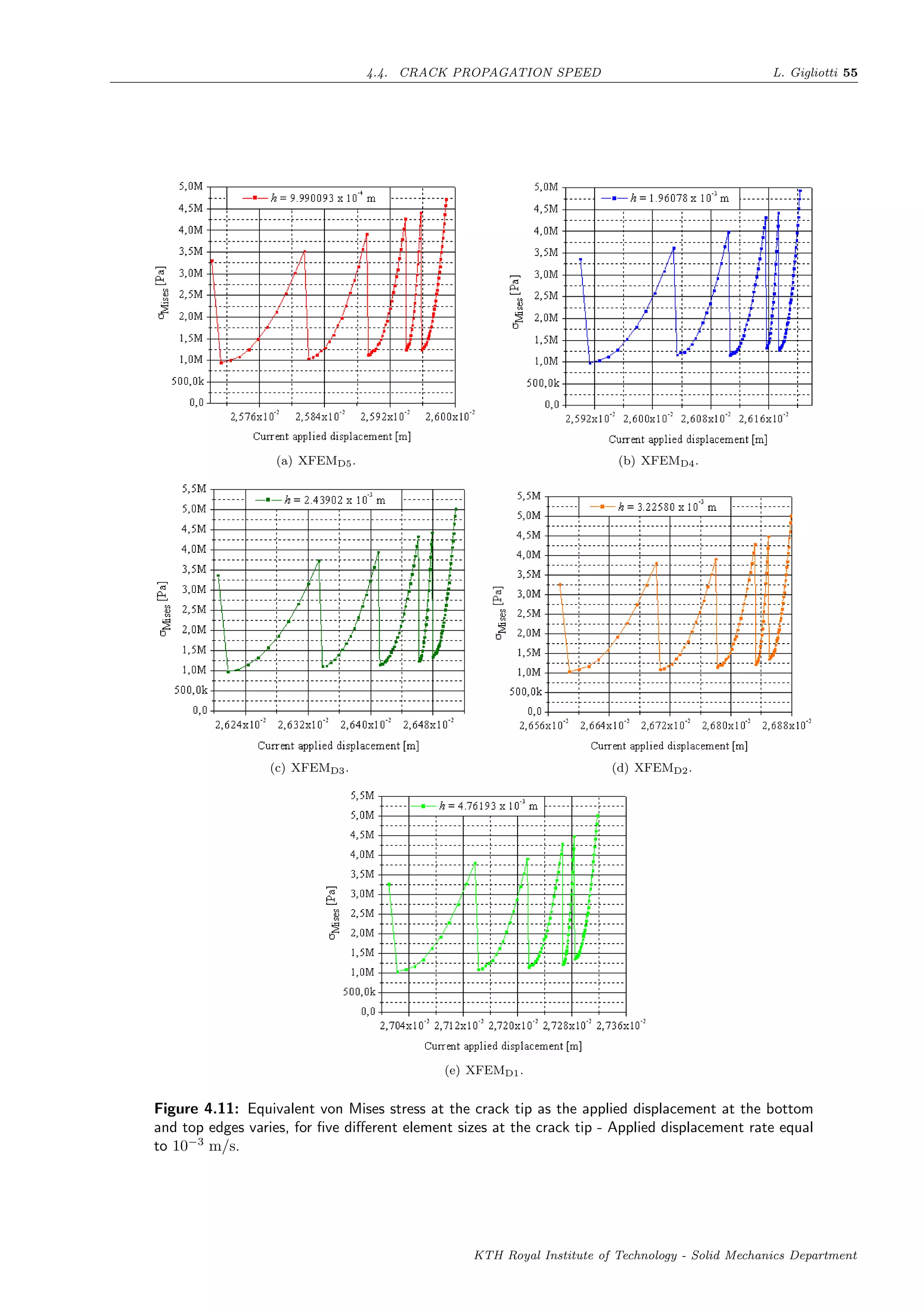
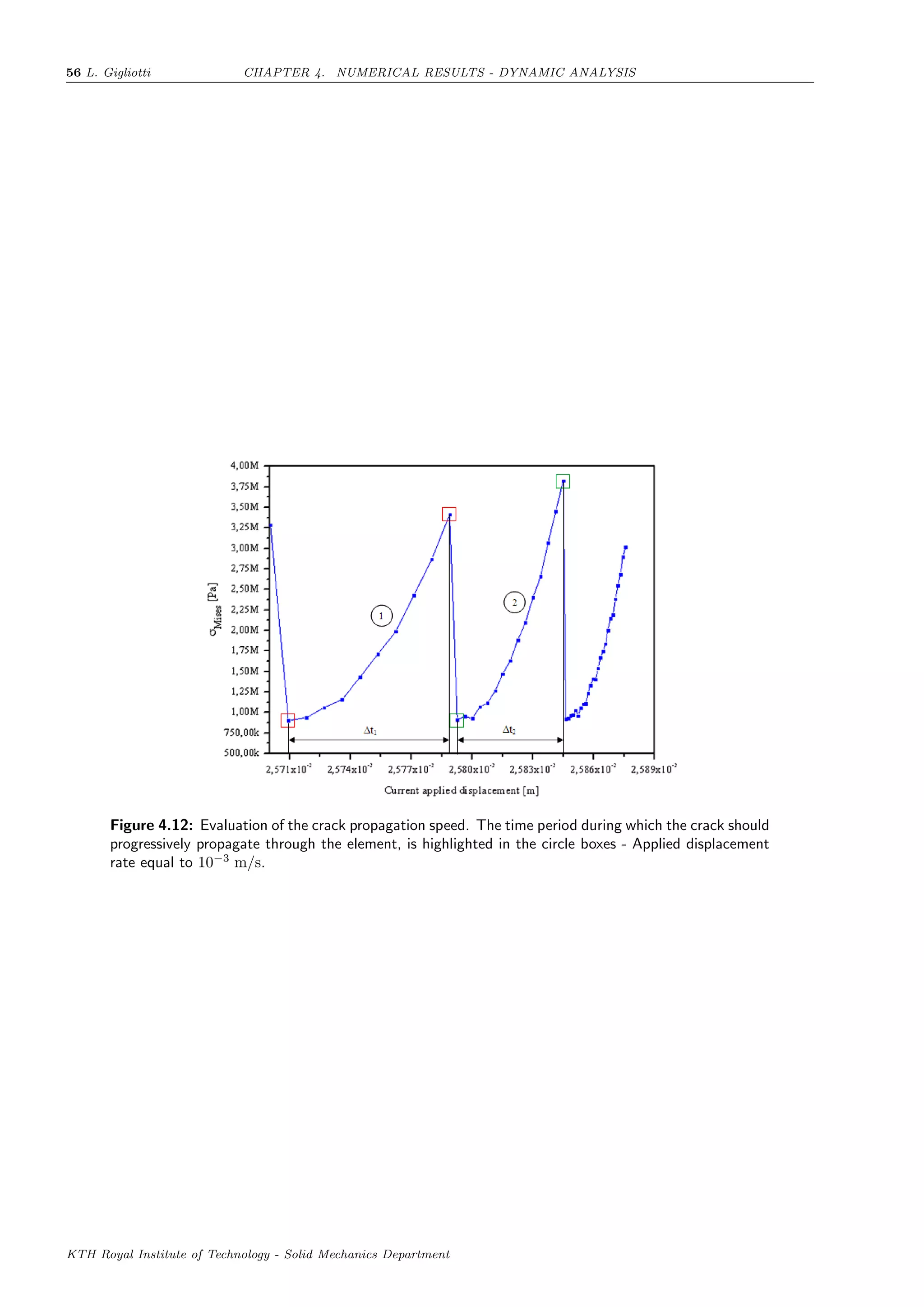
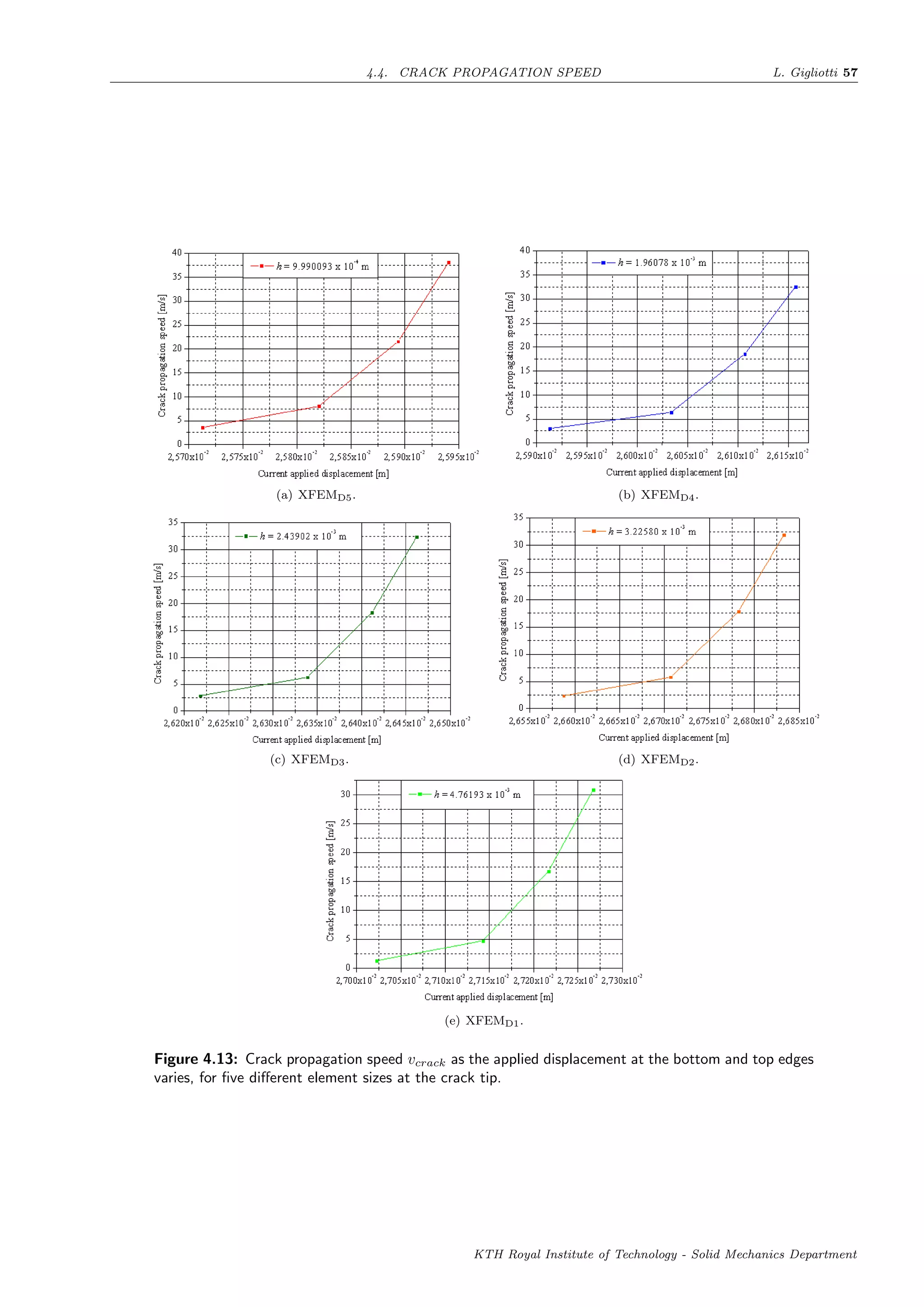
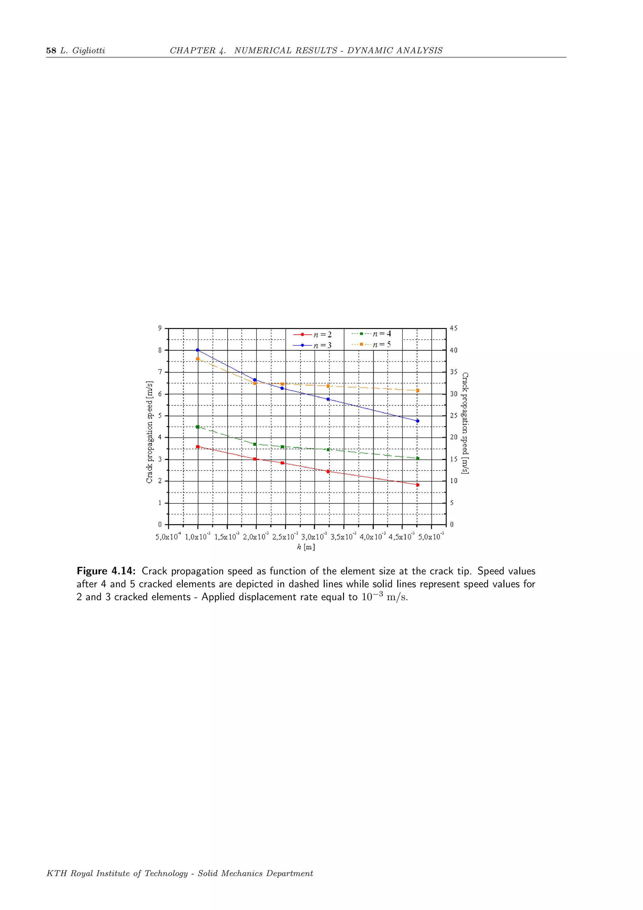
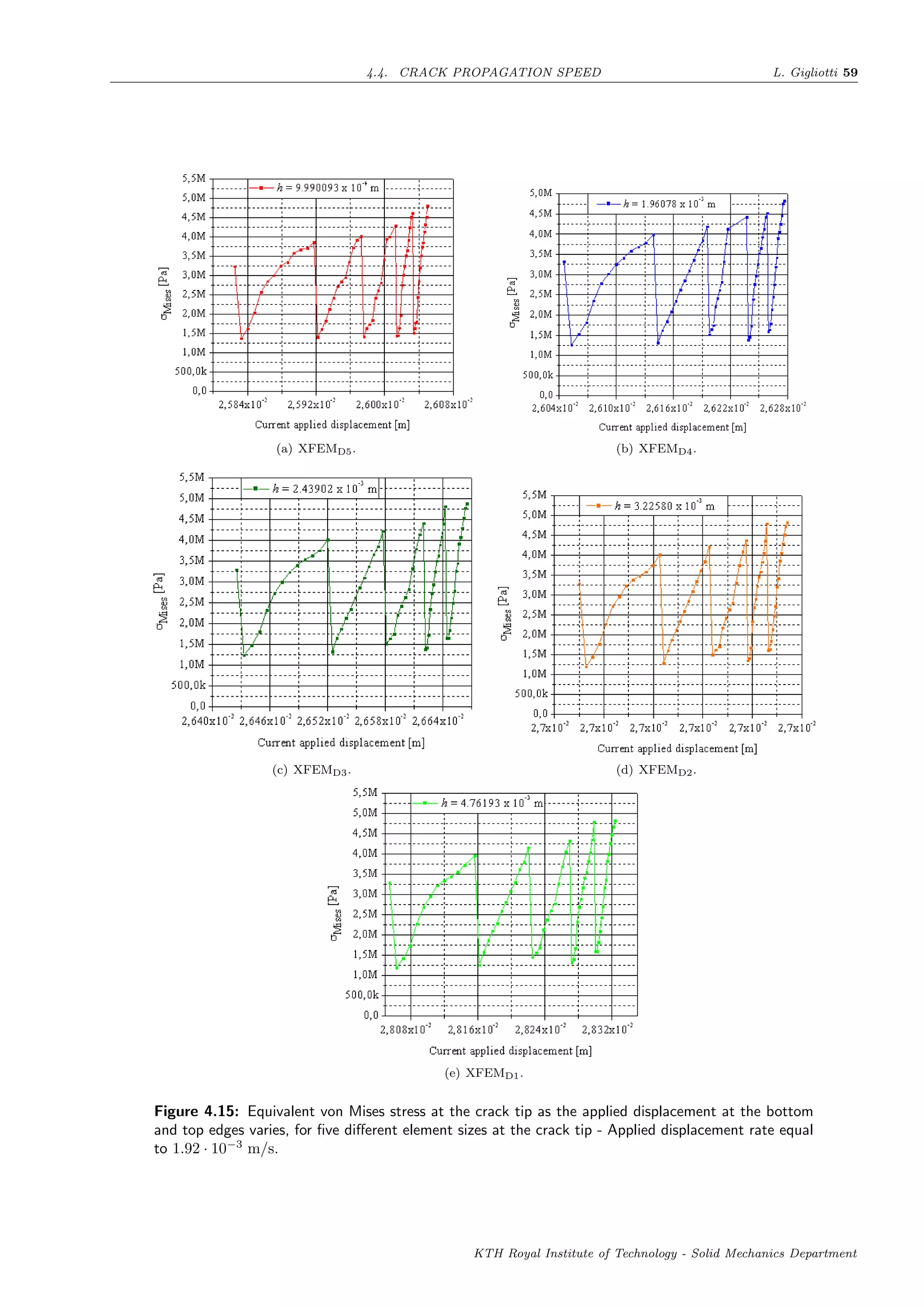
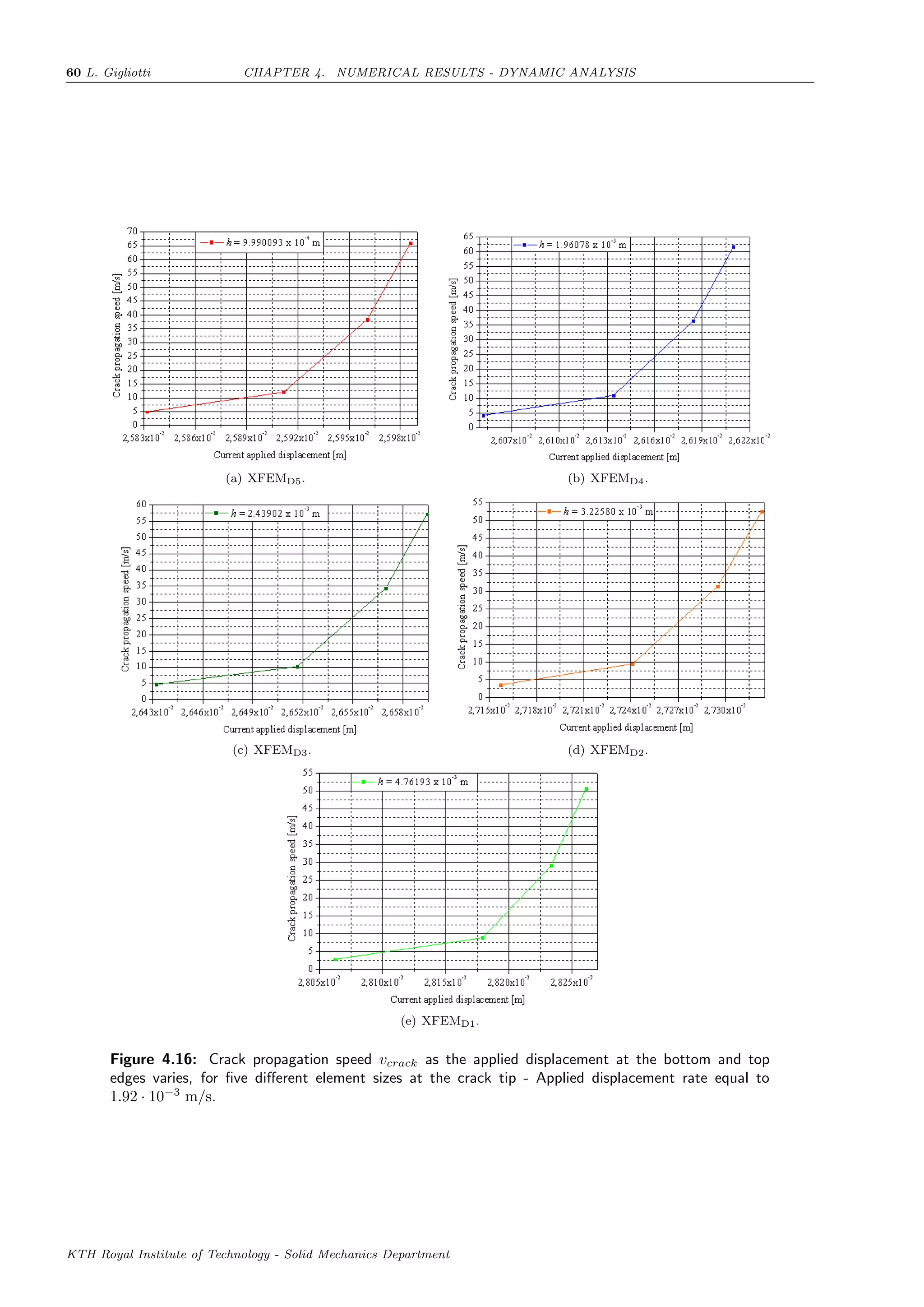
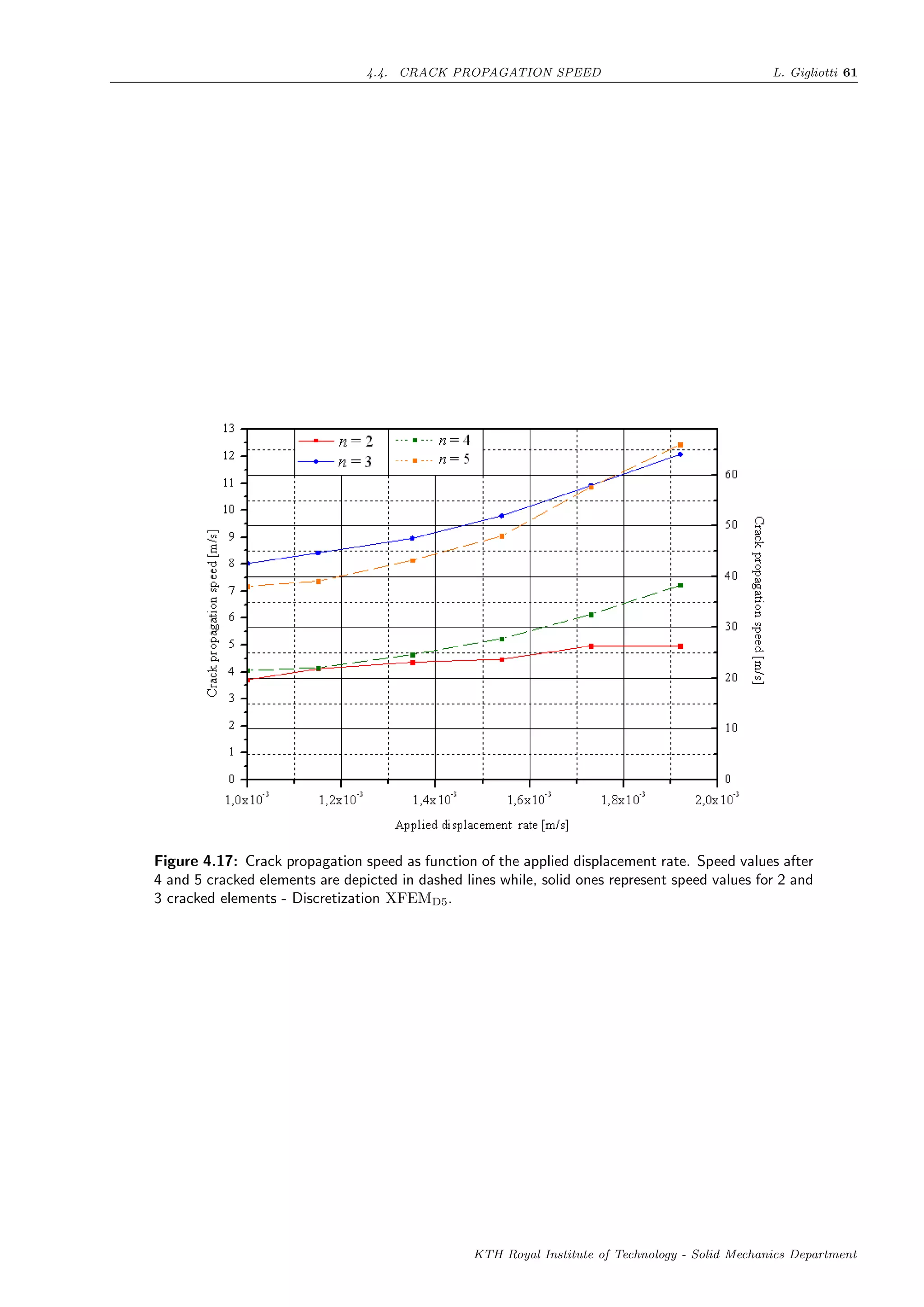
![62 L. Gigliotti CHAPTER 4. NUMERICAL RESULTS - DYNAMIC ANALYSIS
4.5 Remarks on convergence behaviour
As conclusion, it is worthwhile to comment on the convergence behaviour of the performedsimulations. The scenario is the
following one. The complete convergence is achieved only when the finest discretization is used, the applied displacement
rate is maintained equal to 10−3
m/s and the displacement is such that only one element has been completely cracked,
namely 2.8 · 10−2
m and 2.6 · 10−2
m, for the 45o
mixed-Mode and for the 30o
mixed-Mode, respectively. In all other
cases, it has been not possible to complete the simulations successfully. Moreover, the analysis of residuals, clearly
reveals that the time step increments remain constant to their initial value until the crack propagation criterion (Cfr.
Sec. 2.5) is not satisfied. At this point, the time step increments sharply decrease for two reasons: firstly, it can happens
that convergence is not obtained within the maximum number of iterations allowed for a single step or, secondly, the
computed rate of convergence is too low and the convergence is judged unlikely.
Successively, the appropriate value of the time step increment is reached and thus the simulation can proceed. It
has to be stressed that this value is much smaller than those observed before the crack starts to propagate. During
the crack growth process, the aforementioned time-length of the step increment is kept almost constant and no relevant
variations are observed. Such condition holds until, suddenly, a second sharp decrease in terms of time step increment
occurs. However, at this point this latter is already small enough and a further reduction makes the simulation to exit
automatically with an error. The one described above, is the list of subsequent events occurring in all the carried out
simulations, with no exceptions.
Such difficulties might stem from the limited capacity of most of the elements to sustain distortion without causing
a degradation of performance or failure. These limitations to deal with large distortions are particularly evident in the
case of nonlinear analyses, including large deformations and material nonlinearities, performed with Lagrangian meshes.
Thus, the XFEM implementation is thought to further reduce the element capabilities to tolerate large distortions.
An efficient method to circumvent such shortcomings, or at least to reduce them, is to extend the XFEM capabilities
to the Arbitrary Lagrangian Eulerian formulation [106, 107, 108, 109]. Often, the main cause of the failure of simulations
is the excessive value of distortion of the elements nearby the crack tip; this would require a remeshing procedure,
which is not permitted when XFEM technique is used8
. Meanwhile material motions does not lead to any distortion
in Eulerian finite elements. However, the treatment of constitutive equations and of moving boundaries and interfaces,
e.g. crack surfaces is cumbersome with pure Eulerian finite elements. The ALE formulation is an hybrid technique in
which the advantages of both Lagrangian and Eulerian formulations are combined, while trying to limit as far as possible
their relative disadvantages. It is opinion of the author of this thesis that, the extension of XFEM capabilities to the
ALE formulation in Abaqus/Standard could represent a major step forward to enhance the capabilities of the XFEM
technique to model the crack growth process in materials that can undergo large deformations.
Furthermore, consider the convergence behaviour of iterations performed with the Newton-Raphson method. Roughly
speaking, fundamental conditions for a quadratic rate of convergence ought to be satisfied, i.e. a sufficient smoothness
of the Jacobian matrix J as function of u is needed and, moreover, J should be regular and well conditioned over the
whole domain in the displacement space of the iterative procedure.
It is straightforward to observe that, both such conditions are not met in the problem at hand. In particular, it is
evident that the Jacobian matrix is not only a non-smooth function of u but actually is a discontinuous one within the
enriched elements9
. Therefore, the regularity condition is also not satisfied for the enriched elements. Such considerations
are thought to be among the principal reasons of the lack of convergence faced for the crack propagation analysis.
It has been verified that the Arruda-Boyce material model employed in this section, is stable over the entire considered
range of strains. However, material instabilities may rise also in presence of a localized growth of deformation, as that one
occurring at the crack tip during crack propagation processes. Such phenomenon is known in literature as localization.
This localization phenomenon, results in the formation of slender bands of intense deformation called shear bands10
,
which can be interpreted as the result of material instability in the shear component. Analogously, fracture can be
seen as the result of material instability in the normal direction to the discontinuity surfaces in pure Mode-I or in the
tangential direction in pure Mode-II.
As highlighted in [37], fracture cannot be numerically modeled without difficulties. Indeed, such phenomenon includes
most of the shortcoming related to material instabilities, i.e. localization to a set of measure for rate-independent material
models, zero energy dissipation11
as well as absence of a length scale. The Abaqus/Standard implementation of XFEM
is thought to be still not able to handle such problems.
Analogous convergence difficulties to those encountered in this work, have been faced in [91]. However, in such work,
these shortcoming have been circumvented by adopting a modified scheme of the Newton-Raphson method. It stands to
reason, given the purpose of the present work, such approach has not be here employed.
In [72], has been observed that the convergence rate for the classical XFEM method is of the order
√
h. In addition
to this, in [110] and [111] detailed analyses of the convergence of assumed strain methods have been performed, in the
cases of compressible and incompressible materials. The established a priori error estimate for displacements leads to
a linear rate of convergence. Further works dealing with the rate of convergence for hybrid elements can be found in
literature [112] [113].
All in all, the severe convergence difficulties encountered are reasonably ascribable to the coexistence of several
factors, i.e. fracture mechanics problem, high level of deformation, plane strain conditions, complex material model,
8In addition, the main peculiarity of the XFEM technique would be not exploited.
9Recall Eq. 1.102 and that
dH(x)
dx
= δ(x), where δ(x) is the Dirac delta function.
10The name shear bands stems from the fact that often the deformation mode in these bands of high deformation is shear.
11This, in particular, is thought to be the most relevant drawback, since fracture process leads to significant energy dissipation.
KTH Royal Institute of Technology - Solid Mechanics Department](https://image.slidesharecdn.com/5bffcdff-873e-4f02-b330-da222b639ff8-151115100138-lva1-app6891/75/FULLTEXT01-68-2048.jpg)


![Bibliography
[1] Ibrahimbegovic, A., Nonlinear Solid Mechanics: Theoretical Formulation and Finite Element Solution Methods,
Springer, 2008.
[2] Holzapfel, G.A., Nonlinear Solid Mechanics: A Continuum Approach for Engineering, John Wiley & Sons Ltd,
Chichester, 2000.
[3] Treloar, L.R.G., The Physics of rubber elasticity, 3rd
edition, Clarendon Press, Oxford,1975.
[4] Ogden, R.W., Large Deformation Isotropic Elasticity - On the Correlation of Theory and Experiment for Incom-
pressible Rubberlike Solids, Proceedings of the Royal Society of London. Series A, Mathematical and Physical
Sciences, 1972, A326 (1567), 565-584.
[5] Ogden, R.W., The elasticity of a network of long chain molecules. I and II, Transactions of the Faraday Society,
1943, 39, 36-41 and 241-246.
[6] Rivlin, R.S., Large elastic deformations of isotropic materials. IV. Further developments of the general theory,
Philosophical Transactions of the Royal Society of London, 1948, A241 (835), 379-397.
[7] Ogden, R.W., Non-linear elastic Deformations, Dover, New York, 1997.
[8] Flory, P.J., Principles of Polymer Chemistry, Cornell University Press, Ithaca, 1953.
[9] Flory, P.J., Statistical Mechanics of Chain Molecules, Interscience, 1969.
[10] Kuhn, R.S., Grun, F., Beziehungen zwischen elastischen Konstanten und Dehnungsdoppelbrechung hochelastischer
Stoffe, Kolloid-Zeitschrift, 1942, 101, 248-271.
[11] Mooney, M., A theory of large elastic deformation, Journal of Applied Physics, 1940, 11(9), 582-592.
[12] Treloar, L.R.G., A theory of large elastic deformation, Transaction of Faraday Society, 1944, 40, 59-70.
[13] Jones, D.F., Treloar, L.R.G., The properties of rubber in pure homogeneous strain, Journal of Physics D: Applied
Physics, 1944, 8 (11), 007, 1285-1304.
[14] Arruda, E.M., Boyce, M.C., A three-dimensional constitutive model for the large stretch behaviour of rubber elastic
materials, Journal of the Mechanics and Physics of Solids, 1993, 41 (2), 389-412.
[15] Mark, J.E., Erman, B., Rubberlike Elasticity a Molecular Primer, John Wiley & Sons Ltd, New York, 1993.
[16] Yeoh, O.H, Characterization of elastic properties of carbon black-filled rubber vulcanizates, Rubber Chemistry and
Technology, 1990, 63 , 792-805.
[17] Kawabata, S., Kawai, H., Strain energy density functions of rubber vulcanizates from biaxial extension, Advances
in Polymer Science, 1977, 24, Springer-Verlag, Berlin, 90-124.
[18] Seki, W., Fukahori, Y., Iseda, Y., Matsunaga, T., Large-deformation finite-element analysis for multilayer elas-
tomeric bearings, Rubber Chemistry and Technology, 1987, 60, 856-869.
[19] Gent, A.N., A new constitutive relation for rubber, Rubber Chemistry and Technology, 1996, 69, 59-61.
[20] Kilian, H.G., Equation of State of Real Networks, Polymer, 1981, 22, 209-216.
[21] Rivlin, R.S., Thomas, A.G., Rupture of rubber I. Characteristic energy for tearing, Journal of Polymer Science
1952, 10(3), 291-318.
[22] Griffith, A.A., The phenomena of rupture and flow in solids, Philosophical Transactions of the Royal Society A:
Mathematical, Physical and Engineering, Delft, 1921, 221, 163-197.
[23] Griffith, A.A., The theory of rupture, Proceedings of First International Congress of Applied Mechanics, Eds.
Biezeno and Burgers, Waltman, 1924, 55-63.
[24] Irwin, G.R., Kies, J., Fracturing and fracture dynamics, Welding Journal Research Supplement, 1952.
[25] Orowan, E., Fundamentals of brittle behaviour of metals, Fatigue and Fracture of Metals, John Wiley & Sons Ltd,
New York, 1993, 139-167.
[26] Irwin, G.R. Fracture, Handbook of Physics, 1958, 6, 551-590.
[27] Gdoutos, E.E., Daniel, I.M., Schubel, P., Fracture mechanics of rubber, Mechanics, Automatic controls and
Robotics, Facta Universitatis 2003, 3(13), 497-510.
67](https://image.slidesharecdn.com/5bffcdff-873e-4f02-b330-da222b639ff8-151115100138-lva1-app6891/75/FULLTEXT01-73-2048.jpg)
![68 L. Gigliotti BIBLIOGRAPHY
[28] Procedures of Army Symposium on Solid Mechanics - Case Studies on Structural Integrity and Reliability, AMMRC
MS 78-3 1978, Army Materials and Mechanic Research Center.
[29] Stevenson, A., A fracture mechanics study of the fatigue of rubber in compression, International Journal of
Fracture, 1983, 23, 47-59.
[30] Greensmith, H.W., Rupture of Rubber. Part 8: Comparisons of Tear and Tensile Rupture Measurements, Journal
of applied Polymer Science, 1960, 21, 175.
[31] Lindley, P.B., Engineering Design with Natural Rubber, MRPRA, 1974.
[32] Lindley, P.B., Fatigue and Fracture of Elastomers, Master Thesis Report TVSM-5078, University of Lund 1998.
[33] Zienkiewicz, O.C., Taylor, R.L., The Finite Element Method, Vols. 1-3, Butterworth-Heinemann, Oxford 2000.
[34] http://homepage.usask.ca/~ijm451/finite/fe_resources/node139.html
[35] Atluri, S.N., Computational methods in mechanics - Vol.2 Computational methods in the mechanics of fracture,
Mechanics and Mathematics Methods, North-Holland 1986.
[36] Liebowitz, H., Sandhu, J.S., Lee, J.D. Menandro, F.C.M., Computational fracture mechanics: research and ap-
plication, Engineering fracture mechanics, 1995, 50, 653-670.
[37] Belytschko, T., Liu, W.K., Moran, B., Nonlinear Finite Element methods for Continua and Structures, John
Wiley & Sons Ltd, Chichester 2000.
[38] Tong, P., Pian, T.H., On the convergence of finite element method for problems with singularities, International
Journal of Solid Structures, 1973, 9, 313-321.
[39] Henshell, R., Shaw, K., Crack tip finite elements are unnecessary, International journal of numerical methods in
engineering, 1975, 9, 495-507.
[40] Benzley, S.E., Representation of singularities with isoparametric finite elements, International journal of numerical
methods in engineering, 1975, 8, 537-545.
[41] Gifforrd, J., Hilton, P., Stress intesity factors by enriched finite elements, Engineering Fracture Mechanics, 1978,
10, 485-496.
[42] Sneddon, I., Integral transform methods, Method of analysis adn solutions of crack problems,
Nordho International, Leyden, 1973.
[43] Newman, J., An improved method of collocation for the stress analysis of cracked plates with various shaped
boundaries, Technical Report TN D-6376, NASA, 1971.
[44] Obata, M., Nemat-Nasser, S., Gata, Y., Branched cracks in anisotropic elastic solids, Journal of applied mechanics
transactions ASME, 1989, 56(4), 858-864.
[45] Chen, Y., Hasebe, N., New integration scheme for the branch crack problem, Engineering Fracture Mechanics,
1995, 52(2), 791-801.
[46] Cruse, T., Boundary element analysis in computational mechanics, Kluwer, Dordrecht, 1988.
[47] Nisitani, H., Body force method for determination of the stress intensity factor, Journal of Aeronutical Society of
India, 1997, 37, 21-41 [Special Issue in Fracture Mechanics].
[48] Babuˇska, I., Banerjee, U., Osborne, E.J., Survey of meshless and generalized finte element methods: A unified
approach, Acta Numerica, 2003.
[49] Belytschko, T., Krongauz, Y., Organ, D., Fleming, M., Krysl, P., Meshless method: An overview and recente
developments,Computer Methods for Applied Mechanical Engineering, 1996, 139, 3-47.
[50] Belytschko, T., Lu, Y., Gu, L., Element-free Galerkin methods, International journal of numerical methods in
engineering, 1994, 37, 229-256.
[51] Fleming, M., Chu, Y.A., Moran, B., Belytschko, T., Enriched element-free Galerkin methods for crack tip fields
Element-free Galerkin methods,International journal for numerical methods in engineering, 1997, 40(8), 1483-
1504.
[52] Oliver, J., Continuum modeling of strong discontinuities in solid mechanics using damage models, Computational
Mechanics Journal, 1995, 17, 49-61.
[53] Rashid, M., The arbitrary local mesh refinement method: an alternative to remeshing for crack propagation
analysis, Computational methods for applied mechanical engineering, 1998, 154, 133-150.
[54] Mohammadi, S., Extended Finite Element Method for Fracture Analysis of Structures, Blackwell Publishing Ltd,
Oxford, 2008.
[55] Abdelaziz, Y., Hamouine, A., A survey of the extended finite element method, Computers and Structures, 2007,
86, 1141-1151.
[56] Karihaloo, B.L., Xiao, Q.Z., Modelling of stationary and growing cracks in FE framework wothout remeshing: a
state-of-the-art review, Computers and Structures, 2003, 81, 119-129.
[57] Melenk, J.M., Babuˇsska, I., The partition of unity finite element method: basic theory and applications, Compu-
tational methods for applied mechanical engineering, 1996, 139, 289-314.
KTH Royal Institute of Technology - Solid Mechanics Department](https://image.slidesharecdn.com/5bffcdff-873e-4f02-b330-da222b639ff8-151115100138-lva1-app6891/75/FULLTEXT01-74-2048.jpg)
![BIBLIOGRAPHY L. Gigliotti 69
[58] Gasser, T.C., Holzapfel, G.A., Modeling 3D crack propagation in unreinforced concrete using PUFEM, Computa-
tional methods for applied mechanical engineering, 2005, 194, 2859-2896.
[59] Strouboulis, T., Copps, K., The generalized finite element method, Computational methods for applied mechanical
engineering, 2001, 190, 4081-4193.
[60] Duarte, C., Babuˇska, I., Pden, J., Generalized finite element methods for three dimensional structural mechanics
problems, Computers and structures, 2000, 77, 215-232.
[61] Belytschko, T., Black, T., Elastic crack growth in finite elements with minimal remeshing, International Journal
for Numerical Methods in Engineering, 1999, 45, 601-620.
[62] Dolbow, J., An extended finite element method with discontinuous enrichment for applied mechanics, PhD Thesis,
Northwestern University, 1999.
[63] Dolbow, J., M¨oes, N., Belytschko, T., Discontinuous enrichment infinite elements with a partition of unity method,
Finite Elements in Analysis and Design, 2000, 36(3-4), 235-260.
[64] M¨oes, N., Dolbow, J., Belytschko, T., A finite element method for crack growth without remeshing, International
Journal for Numerical Methods in Engineering, 1999, 46, 131-150.
[65] Sukumar, N., M¨oes, N., Moran, B., Belytschko, T., Extended finite element method for three dimensional crack
modelling, International Journal for Numerical Methods in Engineering, 2000, 48, 1549-1570.
[66] Belytschko, T., M¨oes, N., Usui, S., Parimi, C., Arbitrary discontinuities in finite elements, International Journal
for Numerical Methods in Engineering, 2001, 50, 993-1013.
[67] Stolarska, M., Chopp, D.L., M¨oes, N., Belytschko, T., Modelling crack growth by level sets in the extended finite
element method, International Journal for Numerical Methods in Engineering, 2001, 51, 943-960.
[68] Osher, S., Sethian, J., Fronts propagating with curvature dependent speed: algorithms based on Hamilton-Jacobi
formulations, Journal of Computational Physics, 1988, 89(1), 12-49.
[69] Ventura, G., Budyn, E., Belytschko, T., Vector level sets for description of propagating crack in finite elements,
International Journal for Numerical Methods in Engineering, 2003, 58, 1571-1592.
[70] Sukumar, N., Chopp, D.L., Moran, B., Extended finite element method and fast marching method for three-
dimensional fatigue crack propagation, Engineering Fracture Mechanics, 2003, 70, 29-48.
[71] Chopp, D.L., Sukumar, N., Fatigue crack propagation of multiple coplanar cracks with the coupled extended finite
element/fast marching method, International Journal for Engineering Science, 2003, 41, 845-869.
[72] Laborde, P., Pommier, J., Renard, Y., Sala¨un, M., High-order finite element method for cracked domains, Inter-
national Journal for Numerical Methods in Engineering, 2005, 64, 354-381.
[73] Stazi, F.L., Budyn, E., Chessa, J., Belytschko, T., An extended finite element method for crack problems with
curvature, Computational Mechanics, 2003, 31, 38-48.
[74] Ventura, G., On elimination of quadrature subcells for discontinuous functions in the extended finite element
method, International Journal for Numerical Methods in Engineering, 2006, 66, 761-795.
[75] Chessa, J., Wang, H., Belytschko, T., On the construction of blending elements for local partition of unity enriched
finite elements, International Journal for Numerical Methods in Engineering, 2003, 57, 1015-1038.
[76] Chessa, J., The XFEM for free surface and two phases flow problems, Dissertation, Northwestern University,
2003.
[77] Fries, T.P., A corrected XFEM approximation without problems in blending elements, International Journal for
Numerical Methods in Engineering, 2008, 75, 503-532.
[78] Bathe, K.J., Finite Element Procedures, Prentice-Hall, Englewood Cliffs, NJ, 1996.
[79] Hu, H., On some variational principles in the theory of elasticiy and the theory of plasticity, Scientia Sinica, 1955,
4, 33-54.
[80] Washizu, K., Variational methods in elasticity and plasticity, Pergamon Press, 3rd
Ed., 1982.
[81] Xiao, Q.Z., Karihaloo, B.L., Improving the accuracy of XFEM crack tip fields using higher order quadrature
and statically admissible stress recovery, International Journal for Numerical Methods in Engineering, 2008, 66,
1378-1410.
[82] Bechet, E., Minnebo, H., M¨oes, N., Burgardt, B., Improved implementation and robustness study of the XFEM
method for stress analysis around crack, International Journal for Numerical Methods in Engineering, 2008, 64(8),
1033-1056.
[83] Charrier, P., Kuczynski, E.O., Verron, E., Marckmann, G., Gornet, L., Chagnon, G., Theoretical and numeri-
cal limitations for the simulation of crack propagation in natural rubber componenents, Constitutive Models for
Rubber III, Busfield & M¨uhr (Eds) 2003.
[84] Timbrell, C., Wiehahn, M., Cook, G., Simulation of crack propagation in rubber, Constitutive Models for Rubber
III, Busfield & M¨uhr (Eds) 2003.
KTH Royal Institute of Technology - Solid Mechanics Department](https://image.slidesharecdn.com/5bffcdff-873e-4f02-b330-da222b639ff8-151115100138-lva1-app6891/75/FULLTEXT01-75-2048.jpg)
![70 L. Gigliotti BIBLIOGRAPHY
[85] Wagner, G.J., M¨oes, N., Liu, W.K., Belytschko T., The extended finite element method for rigid particles in Stokes
flow, International Journal for Numerical Methods in Engineering, 2001, 51, 293-313.
[86] Wells, G.N., de Borst, R., Sluys, L.J., A consistent geometrically non-linear approach for delamination, Interna-
tional Journal for Numerical Methods in Engineering, 2002, 54(9), 1333-1355.
[87] Hughes, T.J.R., Tezduyar, T.E., Finite elements based upon Midlin plate-theory with particular reference to the
4-node bilinear isoparametric element, Journal of Applied Mechanics, 1981, 48(3), 587-596.
[88] Dolbow, J., M¨oes, N., Belytsckho, T., Modeling fracture in Midlin-Reissner plates with the extended finite element
method, International Journal of Solids and Structures, 2000, 37, 587-596.
[89] Legrain, G., M¨oes, N., Verron, E., Stress analysis around crack tips in finite strain problems using the eXtended
finite element method, International Journal for Numerical Methods in Engineering, 2005, 63, 290-314.
[90] Dolbow, J.E., Devan, A., Enrichment of enhanced assumed strain approximations for representing strong dis-
continuities: addressing volumetric incompressibility and the discontinuous patch test, International Journal for
Numerical Methods in Engineering, 2004, 59, 47-67.
[91] Kroon, M., Dynamic steady-state analysis of crack propagation in rubber-like solids using an extended finite
element method., Computational Mechanics, 2012, 49(1), 73-86.
[92] Hibbit, D., Karlsson, B., Sorensen, P., Inc. ABAQUS/Standard User’s Manual, Ver. 6.10, Pawtucket, Rhode
Island, 2004.
[93] Dassault Syst`emes, Abaqus 6.9 Overview - June 2009, 2009, available at http://abaqusdoc.ucalgary.ca/v6.9/
books/rnb/default.htm
[94] Hansbo, A., Hansbo, P., A finite element method for the dimulations of strong and weak discontinuities in solid
mechanics, Computer Methods in Applied Mechanics and Engineering, 2004, 193, 3524-3540.
[95] Song, J.H., Areias, P.M.A., Belytsckho, T., A method for dynamic crack and shear band propagation with phantom
nodes, International Journal for Numerical Methods in Engineering, 2006, 67, 868-893.
[96] http://www.matthewpais.com/abaqus
[97] Giner, E., Sukumar, N., Tarancon, J., Fuenmayor, F., An Abaqus implementation of the eXtended Dinite Element
Method, Engineering Fracture Mechanics, 2009, 76(3), 347-368.
[98] Benzeggagh, M.L., Kenane, M., Measurement of Mixed-Mode delamination Fracture Toughness Unidirectional
Glass/Epoxy composites with Mixed-Mode bending apparatus, Composites Science and Technology, 1996, 56, 439-
449.
[99] Krueger, R., The Virtual Crack Closure Technique: History, Approach and Applications, NASA/CR-2002-211628,
ICASE Report No.2002-10, 2002.
[100] Pais, M.J., Variable amplitude fatigue analysis using surrogate models and exact XFEM analysis, PhD Disserta-
tion, University of Florida, 2011.
[101] Stephenson, R.A., The equilibrium field near the tip of a crack for finite plane strain of incompressible elastic
materials, Journal of Elasticity, 1982, 12(1), 65-99.
[102] Hilbert, H.M., Hughes, T.J.R., Taylor, R.L., Improved numerical dissipation for time integration algorithms n
structural dynamics, Easrthquake Engineering and Structural Dynamics, 1977, 5, 283-292.
[103] Grossberg, R., Lessmann, O., Remarks on local stability and the local order property, Department of Mathematical
Sciences, Carnegie Mellon University, 1988, Reserch report No. 98-220., available at http://repository.cmu.
edu/math/626
[104] Czekanski, A., El-Abbasi, N., Meguid, S.A., Optimal time integration parameters for elastodynamic contact prob-
lems, Communications in Numerical Methods in Engineering, 2001, 17, 379-384.
[105] Kroon, M., Stedy-state crack growth in rubber-like solids, International Journal of Fracture, 2011, 169, 49-60.
[106] Belytschko, T., Kennedy, J.M., Computer models for subassembly simulation, Nuclear Engineering Design, 1978,
49, 17-38.
[107] Hughes, T.J.R., Liu, W.K., Zimmerman, T.K., Lagrangian-Eulerian finite element formulation for incompressible
viscous flows, Computer Methods in Applied Mechanics and Engineering, 1981, 29, 329-349.
[108] Liu, W.K., Belytschko, T., Chang, H., An arbitrary Lagrangian-Eulerian finite element method for path-dependent
materials, Computer Methods in Applied Mechanics and Engineering, 1986, 58, 227-246.
[109] Benson, D.J., An efficient, accurate simple ALE method for nonlinear finite element programs, Computer Methods
in Applied Mechanics and Engineering, 1989, 72, 205-350.
[110] Reddy, B.D., Simo, J.C., Stability and convergence of a class of enhanced strain methods, SIAM Journal on
Numerical Analysis, 1995, 32, 1705-1728.
[111] Simo, J.C., Rifai, M.S., A class of assumed strain methods and the method of incompatible nodes, International
Journal for Numerical Methods in Engineering, 1990, 29, 1595-1638.
[112] Lamichhane, P., Reddy, B.D., Wohlmuth, I., Convergence in the incompressible limit of finite element approxi-
mations based on the Hu-Washizu formulation, Journal Numerische Mathematik, 2006, 104(2), 151-175.
[113] Fortin, M., An analysis of the convergence of mixed finite element methods, RAIRO - Analyse num´erique, 1977,
11(4), 341-354.
KTH Royal Institute of Technology - Solid Mechanics Department](https://image.slidesharecdn.com/5bffcdff-873e-4f02-b330-da222b639ff8-151115100138-lva1-app6891/75/FULLTEXT01-76-2048.jpg)