An Improved Ant Colony System Algorithm for Solving Shortest Path Network Problems.pdf

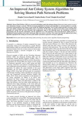
International Journal of Science and Research (IJSR)
ISSN: 2319-7064
Index Copernicus Value (2016): 79.57 | Impact Factor (2017): 7.296
Volume 7 Issue 12, December 2018
www.ijsr.net
Licensed Under Creative Commons Attribution CC BY
An Improved Ant Colony System Algorithm for
Solving Shortest Path Network Problems
Douglas Yenwon Kparib1
, Stephen Boakye Twum2
, Douglas Kwasi Boah3
Department of Mathematics, Faculty of Mathematical Sciences, University for Development Studies, Post Office Box 24 – Navrongo
(Ghana)
Abstract: Shortest Path Problems (SPP) are concerned with finding a path with minimum distance from one or more sources to one or
more destinations through a network. With the increasing application of shortest path algorithms to network problems in real life,
researchers and practitioners have begun to look outside the traditional algorithms, such as label setting and label correcting, which
have some deficits compared with an algorithm such as Ant Colony. In this paper, an improved ant colony system meta-heuristic
algorithm for solving SSP has been presented with modifications made in the following areas: the introduction of dynamic
programming into the heuristic information, and the application of a ratio approach to the local pheromone update process. A
hypothetical network problem of ten nodes with twenty edges was used as a test case. The results show that the improved ant colony
algorithm outperforms the existing one in terms of the number of iterations required to converge to optimality.
Keywords: Shortest path, Network, Label-setting, Label-correcting, Ant colony system, Algorithm, Dynamic programming.
1. Introduction
A network is a collection of entities connected by some
relationship, which can be represented as a graph. Shortest
Path Problems (SPP) are concerned with finding a path with
minimum distance from one or more sources to one or more
destinations through a network (Yongtaek et al, 2010;
Paraveen et al, 2013).
Classical examples of SPPs are the Travelling Salesman
Problem (TSP), the Knapsack Problem (KP) and the
Capacitated Vehicle Routing Problem (CVRP). There is
alsoan increasing application of SPP in real life. Researchers
in algorithms for solving SPPs have begun to look outside
the traditional algorithms such as label setting and label
correcting, which have some deficits in handling large scale
and complicated network problems, to novel meta-heuristic
algorithms. To address the stated shortfalls of the exact
algorithms, the ant colony algorithm was introduced by
Dorigo (1992). It has been the focal point for researchers
with the hope of finding a better algorithm for solving large
scale and complicated networks problems (Gulben and
Orhan, 2015). Some current contributors to the literature of
ant colony algorithms are Mikita et al (2014) who
introduced the Elitist strategy and punishment strategy
pheromone update where extra pheromone is added to the
edges that belong to the best paths whilst pheromone are
subtracted from edges belonging to the worst paths per
iteration, Anuj et al (2012) incorporated a genetic algorithm
to the ant colony algorithm, Gulben and Orhan (2015)
developed the ant colony system algorithm with parametric
analysis and Xiaomeng (2016) proposed the pheromone
update increment as the inverse of the pheromone of the path
constructed by the ant.
The current research develops an improved ant colony
system algorithm for solving SPPs. The proposed algorithm
has been applied to a network of ten (10) nodes with 20
edges. Ant colony algorithm is used to solve the problem
because it was primarily designed to handle network
problems and has demonstrated its ability in obtaining the
best solution for large network problems (Gulben and
Orhan, 2015). The ant Colony algorithm was inspired by the
socialist lifestyle exhibited by ants in search of food and
other provisions (Dhiman et al., 2014). They determine the
shortest path from their source of food to nest through a
chemical called pheromone. The ants drop this pheromone
along their paths as they carry the food to the nest. The path
that accumulates more of the pheromone gives the shortest
path. For example in Figure 1, the first ant walks randomly
until it discovers the food source (F); it then returns to the
nest (N), depositing a quantity of pheromone along the path.
Other ants follow one of the paths (as in 2) at random, also
depositing a quantity of pheromone in their trail. As the ants
on the shortest path lay pheromone faster, this path will
contain more pheromone than the other paths, thus making it
more desirable (as in 3) to subsequent ants. Therefore, the
shortest path is likely to be followed by many ants as it is
regularly reinforced with a greater quantity of pheromone.
The pheromone of the longer paths evaporate with time,
therefore making them less attractive to other ants (Syed and
Sindhanaiselvin, 2013).
Figure 1: The behavior of real ants on a path with time
(Syed and Sindhanaiselvan, 2013)
The ant colony algorithm is one in which a number of
artificial ants are considered at each iteration. Iteration refers
to the total number of steps taken by all the ants to
accomplish a feasible solution (Manuel, 2004). Each ant
Paper ID: ART20193716 10.21275/ART20193716 1123

ISSN: 2319-7064
www.ijsr.net
builds a solution by moving from one node to another on the
graph network with the constraint of not coming back to the
same node which it had been to before in its movement
(Gianni, 2004). At each step of the construction of the
solution, the decision of an artificial ant moving from node 𝑖
to node 𝑗 is based on a stochastic process which is
influenced by the pheromone trail, provided node 𝑗 has not
been visited before by the ant (Dorigo et al, 2006).
Like real ant colonies, artificial ant algorithms are made-up
of entities cooperating to find a solution to the problem
under consideration. Although the complex nature of each
artificial ant makes it capable of finding a feasible solution,
high quality solutions are the result of cooperation. Ants
cooperate by means of the information they simultaneously
read on the problem states. Stigmergy is a mechanism of
communication by modifying the environment. Both real
and artificial ants modify some aspects of their environment.
As real ants deposit pheromone on the path they visit,
artificial ants change some numeric information of the
problem states (Dorigo et al, 1999). This information takes
into account the ant’s current performance and can be
obtained by any ant accessing the state. In ant algorithms,
the only means of communication among the ants is by the
pheromone. They affect the way the problem environment is
perceived by the ants as a function of the past history. Also
an evaporation mechanism, similar to real pheromone
evaporation, modifies the pheromone (Blum, 2005). The
objective of both real and artificial ants is to find a shortest
path joining an origin (nest) to destination (food) site. They
both move step-by-step through adjacent states of the
problem. Artificial ants, as real ones, construct solutions by
applying a probabilistic decision to move through adjacent
states (Dhiman et al, 2014).
The three main types of meta- heuristics ACO algorithms
are: (i) Ant System (AS) by Dorigo (1992) (ii) Max-Min Ant
System (MMAS) by Hoos and Stutzle (1996) (iii) Ant
Colony System (ACS) by Dorigo and Gambardella (1997).
The three meta-heuristics ACO algorithms differ by the way
they update the pheromone trail values. The current work is
situated within ACS. In the next section, the characteristics
of the ACS and the modifications for improvement made to
it by the authors is presented; this is followed by a
discussion of a test case. The final section concludes the
paper.
2. The ACS and Improvements
2.1 The Ant Colony System Algorithm
The seven main steps in ACS are: (i) setting parameters (ii)
initializing pheromone trails. (iii) calculating the heuristic
Information. (iv) building of the ant solution by using the
stochastic state transition rule. (v) carrying out the local
pheromone update. (vi) applying local search to improve
solution constructed by an ant. (vii) Updating the global
pheromone information.
Initialization of pheromone: This is the initial pheromone
𝜏𝑖𝑗 (0) that is deposited along the route (𝑖, 𝑗) at the beginning
of the search, which is usually a small positive constant
value. The purpose of the initial pheromone is to make sure
that every edge has at least a little probability of being
selected (Gianni, 2004). The initial pheromone is defined
(see Oto et al, 2014) as:
𝜏𝑖𝑗 (0) =
1
𝑛
where 𝑛 is the number of number nodes.
Heuristic information phase: Heuristic information, known
as visibility measure is an additional information available to
the ant algorithm that helps to streamline the search
procedure: it is usually referred to as a local information.
Heuristic information tells how attractive a route is; which
assists the ants in the construction of shortest path
(Mavrovouniotis PhD thesis, 2013). It is defined as a
reciprocal of the distance between two nodes as:
Pheromone update rule: The updating of pheromone along
a trail is carried out after all the ants have constructed the
solutions. However, different researchers have come up with
other updating schemes. The three aspects under pheromone
update are: the amount of pheromone to be laid, the amount
be evaporated, and the ants that are permitted to lay their
pheromone (Nada, 2009).The two pheromone updates are
the local pheromone update and global pheromone update.
Local Update: The local updating rule is applied on the
edges whilst constructing the solutions, in order to reduce
the quantity of pheromone on them (Nada, 2009). Since its
introduction by Dorigo and Gambardella (1997), a number
of people have come up with different approaches for
calculating it.
Chia-Ho et al (2009) proposed a formula for calculating the
local pheromone update as:
Where 𝜌 is the rate of evaporation of the pheromone along
(𝑖, 𝑗) trail.
Global Update: Global updating is performed by all ants
that have completed their schedule. It is to increase the
content of the pheromone on the path to facilitate the
convergence of the algorithm. Yu et al (2009) proposed a
formula for calculating the pheromone trail increment as:
∆𝜏𝑖𝑗
𝑘
=
𝑄
𝐾 × 𝐿
×
𝐷𝑘
− 𝑑𝑖𝑗
𝑚𝑘 × 𝐷𝑘
𝑖𝑓 𝑙𝑖𝑛𝑘 𝑖, 𝑗 𝑖𝑠 𝑜𝑛 𝑡ℎ𝑒 𝑘𝑡ℎ 𝑟𝑜𝑢𝑡𝑒
0 𝑜𝑡ℎ𝑒𝑟𝑤𝑖𝑠𝑒
where 𝑄 is a constant value; 𝐷𝑘
is length of the 𝑘𝑡ℎ
path
(solution); 𝐿 is the sum of the length of all the paths
generated i.e. 𝐷𝑘
𝑘 ; 𝑘 is the name of the path; 𝑚𝑘
is the
number of customers in the𝑘𝑡ℎ
path; 𝑚𝑘
> 0; 𝐾 is the
number of paths generated and 𝐾 > 0.
Probabilistic Decision Rule phase: In constructing the
feasible solutions, the decision by the ants to move from one
node to the next is based on a stochastic probability rule.
The probabilistic decision rule by Majid et al. (2011) is
given as:
Paper ID: ART20193716 10.21275/ART20193716 1124

ISSN: 2319-7064
www.ijsr.net
𝑃𝑖𝑗
𝑘
𝑡 =
1 𝑖𝑓 {𝑞 ≤ 𝑞0 𝑎𝑛𝑑 𝑗 = 𝑗∗
0 𝑖𝑓 {𝑞 ≤ 𝑞0 𝑎𝑛𝑑 𝑗 ≠ 𝑗∗
𝜏𝑖𝑗 𝑡
𝛼
𝜂𝑖𝑗 𝑡
𝛽
𝜏𝑖𝑟 𝑡
𝛼
𝜂𝑖𝑟 𝑡
𝛽
𝑟∈𝑁𝑖
𝑘
𝑜𝑡ℎ𝑒𝑟𝑤𝑖𝑠𝑒
𝑗∗
: yields arg 𝑚𝑎𝑥𝑟∈𝑁𝑖
𝑘 𝜏𝑖𝑗 𝑡
𝛼
𝜂𝑖𝑗 𝑡
𝛽
and it is used to identify the unvisited node in 𝑁𝑖 that
maximizes 𝑃𝑖𝑗
𝑘
(𝑡) (Majid et al., 2011).
𝑁𝑖
𝑘
∈ 𝑁𝑖 is the set of nodes which are the neighbors of node
𝑖 and are not yet visited by ant 𝑘 (nodes in 𝑁𝑖
𝑘
are obtained
from those in 𝑁𝑖 by the use of ant 𝑘′𝑠private memory
𝐻𝑖
𝑘
(which stores nodes already visited by the ant)).
𝑁𝑖 is the set of nodes which are directly linked to node 𝑖 by
an edge (i.e. the neighbours of node 𝑖).
𝜏𝑖𝑗 𝑡 is the quantity of pheromone trail laid along the edge
linking node 𝑖 and node j.
𝜂𝑖𝑗 𝑡 is the heuristic information for the ant visibility
measure.
𝛼 is the parameter to control the influence of 𝜏𝑖𝑗
𝛽 is the parameter to control the influence of 𝜂𝑖𝑗
𝑞0 is the pre-defined parameter (0 ≤ 𝑞0 ≤ 1).
𝑞is the uniformly distributed random number to determine
the relative importance of exploitation versus exploration,
𝑞 ∈ [0, 1].
2.2 Proposed Improvement ofthe Ant Colony System
Algorithm
The key contributions made to this algorithm falls under
initial pheromone trail, heuristic information, local
pheromone update and global pheromone update. The initial
pheromone trail plays a vital role in the beginning stage of
the construction of solutions by ants. However, the uniform
values used as initial pheromone trails by researchers (e.g.
Blum, 2005) do not fairly discriminate among the routes for
the ants to make an informed choice, resulting in many ants
generating solutions that are far from the best solution.
Therefore, the new initial pheromone trail has been proposed
to address this challenge. They are as follow:
The proposed initial pheromone trail is given as:
𝑛 is the number of nodes (i.e. the size of the problem)
𝐿𝑖𝑗 is the ratio of the distance linking node 𝑖 to node
𝑗, 𝐿𝑖𝑗 =
𝑑𝑖𝑗
𝑑𝑖𝑗
.
Heuristic information tells how attractive a route is, which
assists ants in the construction of shortest path. The heuristic
information in the literature is always calculated based on
the current node, 𝑖 where the ant is and the next node 𝑗.
However, the current approach does not provide the ant with
information on the nature of the path from source to the
current node 𝑖. It is for this reason that, the new heuristic
information has been proposed to solve the problem. Here
the heuristic information is not dependent only on the usual
distance from 𝑖 to 𝑗 but also on the distance from source to 𝑖.
The proposed heuristic information is therefore given as:
where:
𝑑0𝑖 is the minimum distance from the source node to the
present node 𝑖.
𝑑𝑖𝑗 is the distance from node 𝑖 to node 𝑗.
The aim of the local pheromone update is to reduce the
content of the pheromone along the routes to encourage
other ants to generate new paths. However, care has to be
taken so that paths which are far from the optimal are not
created. Therefore, in this new approach, the reduction in the
pheromone level during the construction of paths is such that
smaller quantity is taken from the shortest routes compared
to that taken on longer routes. This departs from the one in
the literature (Chia-Ho et al, 2009) where a constant value is
deducted along all the routes.
The proposed local pheromone trail update is therefore given
as:
Where
The proposed increment pheromone trail update is given as:
In the model for increment in the global update by Yu et al
(2009), K is the number of paths and 𝐿 the sum of the length
of all paths generated and used for updating all the paths no
matter the quality of it. This does not result in quick
convergence to optimality. In the proposed model, the
update is carried out based on the quality of the path
generated. Hence it enhances the speed of the search for
optimal solution.
The proposed increment is therefore given as:
𝑑𝑖𝑗 is the distance of the edge (𝑖, 𝑗)
𝐿𝑘
is the total distance of the 𝑘𝑡ℎ
solution generated by ant k
𝐿 is the ratio of the distance of the feasible solutions
generated.
The probability decision rule is the same as the already
stated one proposed by Majid et al (2011) with the proposed
initial pheromone trail, heuristic information, local
pheromone update trail and global pheromone trail update
embedded in it.
Paper ID: ART20193716 10.21275/ART20193716 1125

ISSN: 2319-7064
www.ijsr.net
3. A Test Problem
Let 𝐺(𝑉, 𝐸) be undirected graph consisting of an indexed set
of nodes V with 𝑛 = 𝑉 and a spanning set of edges (arcs) E
with 𝑚 = 𝐸 , where n and m are the numbers of nodes and
edges (arcs), respectively. Each arc is represented as a pair
of nodes, thus from node𝑖 to node 𝑗, and denoted by (𝑖, 𝑗).
Each arc is associated with distance.
The optimization model with distance as objective is given
as:
subject to: 𝑥𝑖𝑗 ∈ 0, 1 , ∀ 𝑖, 𝑗
where:
𝑑𝑖𝑗 is the distance from node 𝑖to node 𝑗;
𝑥𝑖𝑗 is a binary decision variable.
A network of ten (10) nodes and twenty (20) edges is
considered as shown in Figure 2, which is adopted from
Hillier and Lieberman (2005) with the values modified to be
in line with this work but with the pattern of the connected
nodes maintained. In this example the source node is labeled
1 and the destination node labeled 10. Each edge is
associated with a distance (𝑑𝑖𝑗 ) in kilometers. The values
representing distance are arbitrarily generated. The main aim
here is to find a path from the source to the destination
which minimizes distance, using the optimization model and
the proposed ACS algorithm. The model was run in
MATLAB and a comparison between the proposed ACS and
the existing one (as described earlier) in terms of the number
of iterations required for convergence.
Figure 2: A network of 10 nodes showing the distances between them
3.1 Results and Discussions
Table 1 presents the results of the network problem
considered. In the table, the first and the second columns are
the names of the paths and their composites (path sets)
whereas the third column gives the corresponding distances.
Also, the last row is the number of iterations required by the
existing Ant Colony System Algorithm (E) and the
Improved Ant Colony System Algorithm (I) respectively to
converge to the optimal solution.
Table 1: Results of the network problem considered
Paths Name Path set Distance (km)
𝑃1 1 – 3 – 7 – 8 – 10 18
𝑃2 1 – 2 – 5 – 8 – 10 13
𝑃3 1 – 2 – 5 – 9 – 10 17
𝑃4 1 – 3 – 6 – 8 – 10 15
𝑃5 1 – 3 – 6 – 9 – 10 13
𝑃6 1 – 3 – 5 – 8 – 10 11
𝑃7 1 – 3 – 5 – 9 – 10 15
𝑃8 1 – 2 – 6 – 8 – 10 13
𝑃9 1 – 3 – 7 – 9 – 10 19
𝑃10 1 – 4 – 6 – 8 - 10 17
𝑃11 1 – 4 – 7 – 8 – 10 14
𝑃12 1 – 4 – 5 – 9 – 10 15
𝑃13 1 – 4 – 5 – 8 – 10 11
𝑃14 1 – 2 – 6 – 9 – 10 11
𝑃15 1 – 4 – 6 – 9 – 10 15
𝑃16 1 – 2 – 7 – 9 –10 21
𝑃17 1 – 2 – 7 – 8 – 10 18
The existing ACS takes 140 iterations to converge
to optimal whilst the improved ACS takes 129
From Table 1, the paths 1 – 3 – 7 – 8 – 10(𝑃1) and 1 – 2 – 7
– 8 – 10 (𝑃17)each cover a total distance of 18km. Also, 1 –
2 – 5 – 8 – 10(𝑃2), 1 – 3 – 6 – 9 – 10(𝑃5) and 1 – 2 – 6 – 8 –
10(𝑃8)each have a total distance of 13km. Besides, 1 – 2 – 5
– 9 – 10(𝑃3) and 1 – 4 – 6 – 8 – 10(𝑃10) a total distance of
17km. The same interpretation could be given to the
remaining paths (table). The total minimum distance to be
covered is 11km, associated with the paths 1 – 3 – 5 – 8 – 10
(𝑃6), 1 – 4 – 5 – 8 – 10(𝑃13) and1 – 2 – 6 – 9 –
Paper ID: ART20193716 10.21275/ART20193716 1126

ISSN: 2319-7064
www.ijsr.net
10(𝑃14).Thus, the problem has multi-optimal paths. The
existing ACS algorithm converges to optimality after 140
iterations whilst the improved ACS algorithm takes 129
iterations. Therefore, the improved Ant Colony System
algorithm outperformed the existing one in terms of the
number of iterations required to converge to optimality.
4. Conclusion
Improvements have been made to the existing Ant Colony
System optimization algorithm and the algorithm applied
successfully to a shortest path derived from a hypothetical
network problem. The improved ant colony system
algorithm outperformed the existing ant colony system
algorithm in terms of the number of iterations required to
converge to optimality. Future work would consider a real
network under possibly multi-objective optimization
framework.
References
[1] Anuj, K. G., Harsh, S. and Verma, K. (2012). MANET
Routing Protocols Based on Ant Colony Optimization.
International journal of Modelling and Optimization, 2
(1).
[2] Blum, C. (2005). Review Ant Colony Optimization:
Introduction and Recent Trends. Journal of physics of
life, 2, 353-375, ELSEVIER.
[3] Chia-Ho, C., and Ching-Jung, T. (2009). Applying
Two-Stage Ant Colony Optimization to solve the large
scale Vehicle Routing Problem. Journal of the Eastern
Asia society for Transportation Studies, 8.
[4] Dhiman, P., and Hooda, R. (2014). An Enhanced Ant
Colony Optimization Based Image Edge Detection.
International Journal of Advanced Research in
Computer Science and Software Engineering, 4 (6),
923-933, ISSN 2277128.
[5] Dorigo (1992). Optimization Learning and Natural
algorithms. Unpublished PhD thesis, Dipartimento di
Eletronica, Politecnico di Milano, Italy.
[6] Dorigo, M., and Gambardella, L. M. (1997). Ant Colony
System A Cooperative Learning Approach to the
Travelling Salesman Problem. IEEE Transactions on
Evolutionary Computation, 1 (1), 53-66.
[7] Dorigo, M., Birattari, M., and Thomas Stutzle, T.
(2006). Ant Colony Optimization: Artificial ants as a
computation intelligence technique. IEEE COMP.
INTELL. MAG, (1), 28-39.
[8] Dorigo, M., Caro, G. D., and Gambardella, L.M. (1999).
Ant algorithms for discrete optimization. Artificial life,
5(2), 137-172.
[9] Gianni, D. C. (2004). Ant Colony Optimization and its
Application to Adaptive Routing in Telecommunication
Networks. Unpublished PhD thesis, University of Libre
Bruxelles, Faculty Des Sciences Appliqués 2004.
[10]Gulben, C., and Orhan, Y. (2015). An improved ant
colony optimization algorithm for construction site
layout problems. Journal of building construction and
planning research, 3, 221-232.
[11]Hillier, F. S. and Lieberman, G. (2005). Introduction to
operations research (8th
ed.), McGraw Hill Eighth
Edition.
[12]Majid, Y. K., and Mohammad, S. (2011). An
optimization algorithm for capacitated vehicle routing
problem based on ant colony system. Australian journal
of basic and applied sciences, 5(12), 2729 – 2737, 2011
ISSN 1991 – 8178.
[13]Manuel, L. I. (2004). Multi-Objective Ant Colony
Optimization. Universidad de Granada
(htt://creativecommons.org/licenses/by/2.0/legalcode)
[14]Mavrovounistis, M.(2013). Ant Colony Optimization in
stationary and dynamic Environments. Unpublished
PhD-thesis.
[15]Mikita et al (2014). An Overview of Minimum Shortest
Path Finding System Using Ant Colony Algorithm.
International Journal of Engineering Research and
Technology (IJERT), 3 (1), ISSN 2278-0181.
[16] Nada, M. A. A. S. (2009). Ant Colony Optimization
Algorithm. UbiCC Journal, 4(3), 823-826.
[17]Otoo, D., Amponsah, S. K., and Sebil. C. (2014).
Capacitated clustering and collection of solid waste in
Kwadaso estate, Kumasi. Journal of Asian scientific
research, 4(8), 460 – 472.
[18]Paraveen, S., and Neha, K. (2013). Study of Optimal
Path Finding Techniques. International Journal of
Advancements in Technology, 4 (2), ISSN 0976 – 4860.
[19]Stutzle, T., and Hoos, H. H. (1996). Improving the ant
system: A detailed report on the Max-Min ant system.
ALDA-96-12, FG Intellektik, FB Informatic, TU
Darmstadt, Germany.
[20]Syed, A. K., and Sindhanaiselvan, K. (2013). Ant
colony optimization based routing in wireless sensor
networks. International journal advanced networking
and applications, 4 (04), 1686 – 1689.
[21]Xiaomeng, P. (2016). Application of improved ant
colony algorithm in intelligent medical system from the
perspective of big data. Chemical engineering
transactions, 51, 523-528.
[22]Youngtaek, L. and Sungmo, R. (2010). An efficient
dissimilar path searching method for evacuation routing.
KSCE Journal of civil engineering, 14(1), 61-67.
[23]Yu, B., Zhang, Y. and Yao, B. (2009). An Improved
Ant Colony Optimization for Vehicle Routing Problem.
European Journal of Operational Research,
ELSERVIER.
Paper ID: ART20193716 10.21275/ART20193716 1127

An Improved Ant Colony System Algorithm for Solving Shortest Path Network Problems.pdf

Recommended

Recommended

More Related Content

Similar to An Improved Ant Colony System Algorithm for Solving Shortest Path Network Problems.pdf

Similar to An Improved Ant Colony System Algorithm for Solving Shortest Path Network Problems.pdf (20)

More from Lisa Riley

More from Lisa Riley (20)

Recently uploaded

Recently uploaded (20)

An Improved Ant Colony System Algorithm for Solving Shortest Path Network Problems.pdf