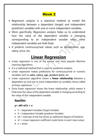
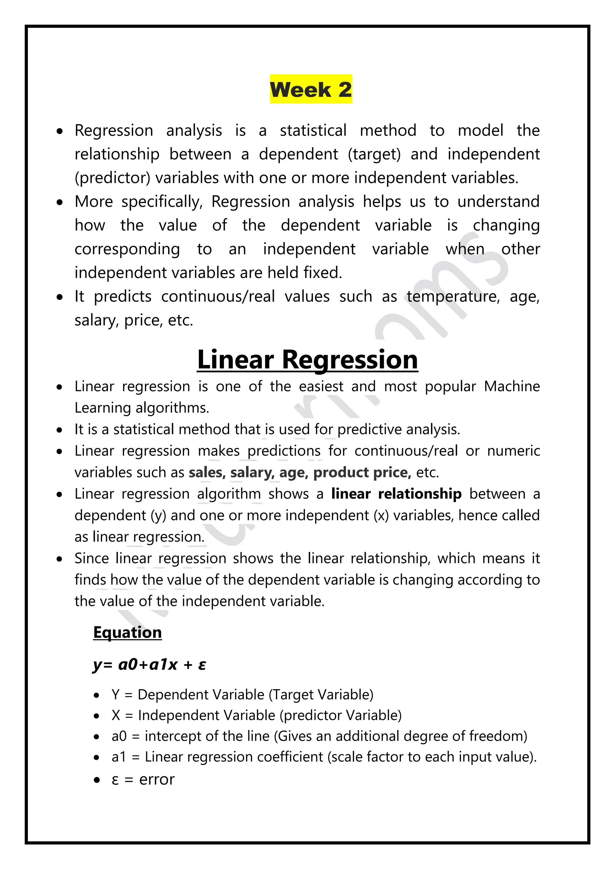
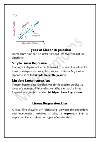
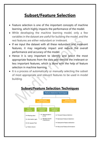
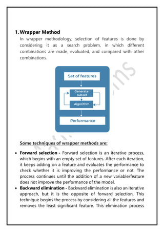
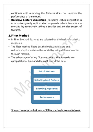
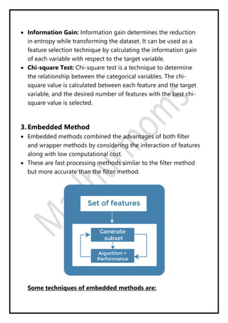
Regression analysis models the relationship between a dependent (target) variable and one or more independent (predictor) variables. Linear regression predicts continuous variables using a linear equation. Simple linear regression uses one independent variable, while multiple linear regression uses more than one. The goal is to find the "best fit" line that minimizes error between predicted and actual values. Feature selection identifies important predictors by removing irrelevant or redundant features. Techniques include wrapper, filter, and embedded methods. Overfitting and underfitting occur when models are too complex or simple, respectively. Dimensionality reduction through techniques like principal component analysis (PCA) transform correlated variables into linearly uncorrelated components.

1. Week 2
 Regression analysis is a statistical method to model the
relationship between a dependent (target) and independent
(predictor) variables with one or more independent variables.
 More specifically, Regression analysis helps us to understand
how the value of the dependent variable is changing
corresponding to an independent variable when other
independent variables are held fixed.
 It predicts continuous/real values such as temperature, age,
salary, price, etc.
Linear Regression
 Linear regression is one of the easiest and most popular Machine
Learning algorithms.
 It is a statistical method that is used for predictive analysis.
 Linear regression makes predictions for continuous/real or numeric
variables such as sales, salary, age, product price, etc.
 Linear regression algorithm shows a linear relationship between a
dependent (y) and one or more independent (x) variables, hence called
as linear regression.
 Since linear regression shows the linear relationship, which means it
finds how the value of the dependent variable is changing according to
the value of the independent variable.
Equation
y= a0+a1x + ε
 Y = Dependent Variable (Target Variable)
 X = Independent Variable (predictor Variable)
 a0 = intercept of the line (Gives an additional degree of freedom)
 a1 = Linear regression coefficient (scale factor to each input value).
 ε = error

2. Types of Linear Regression
Linear regression can be further divided into two types of the
algorithm:
Simple Linear Regression:
If a single independent variable is used to predict the value of a
numerical dependent variable, then such a Linear Regression
algorithm is called Simple Linear Regression.
Multiple Linear regression:
If more than one independent variable is used to predict the
value of a numerical dependent variable, then such a Linear
Regression algorithm is called Multiple Linear Regression.
Linear Regression Line
A linear line showing the relationship between the dependent
and independent variables is called a regression line. A
regression line can show two types of relationship:

3. Positive Linear Relationship:
If the dependent variable increases on the Y-axis and
independent variable increases on X-axis, then such a
relationship is termed as a Positive linear relationship.
Negative Linear Relationship:
If the dependent variable decreases on the Y-axis and
independent variable increases on the X-axis, then such a
relationship is called a negative linear relationship.
Finding the best fit line
 When working with linear regression, our main goal is to find
the best fit line that means the error between predicted values
and actual values should be minimized.
 The best fit line will have the least error.

4.  The different values for weights or the coefficient of lines (a0,
a1) gives a different line of regression, so we need to calculate
the best values for a0 and a1 to find the best fit line, so to
calculate this we use cost function.
Cost function:
The different values for weights or coefficient of lines (a0, a1)
gives the different line of regression, and the cost function is
used to estimate the values of the coefficient for the best fit
line.
Cost function optimizes the regression coefficients or weights.
It measures how a linear regression model is performing.
Mean Squared Error (MSE)
n = Total number of observations
yi = Actual value
(a1xi+a0) = Predicted value {like (mx+c)}
Univariate Regression
 Univariate regression is a statistical technique used to analyse the
relationship between a single independent variable and a single
dependent variable.
 It is a method used to predict the value of a dependent variable
based on the values of a single independent variable.

5. Equation
Y = β0 + β1X + ε
Y is the dependent variable
X is the independent variable
β0 is the intercept or constant
β1 is the coefficient
ε is the error
Multivariate Regression
Multivariate regression is a statistical method used to analyse the
relationship between multiple independent variables and a single
dependent variable.
In other words, it is a technique used to predict the value of a
dependent variable based on the values of two or more
independent variables.
Equation
Y = β0 + β1X1 + β2X2 + β3X3 + ... + βnXn + ε
Y is the dependent variable
X1, X2, X3, ... Xn is the independent variables
β0 is the intercept or constant
β1, β2, β3, ... βn are the coefficients
ε is the error

6. Subset/Feature Selection
 Feature selection is one of the important concepts of machine
learning, which highly impacts the performance of the model.
 While developing the machine learning model, only a few
variables in the dataset are useful for building the model, and the
rest features are either redundant or irrelevant.
 If we input the dataset with all these redundant and irrelevant
features, it may negatively impact and reduce the overall
performance and accuracy of the model.
 Hence it is very important to identify and select the most
appropriate features from the data and remove the irrelevant or
less important features, which is done with the help of feature
selection in machine learning.
 It is a process of automatically or manually selecting the subset
of most appropriate and relevant features to be used in model
building.
Subset/Feature Selection Techniques

7. 1. Wrapper Method
In wrapper methodology, selection of features is done by
considering it as a search problem, in which different
combinations are made, evaluated, and compared with other
combinations.
Some techniques of wrapper methods are:
 Forward selection - Forward selection is an iterative process,
which begins with an empty set of features. After each iteration,
it keeps adding on a feature and evaluates the performance to
check whether it is improving the performance or not. The
process continues until the addition of a new variable/feature
does not improve the performance of the model.
 Backward elimination - Backward elimination is also an iterative
approach, but it is the opposite of forward selection. This
technique begins the process by considering all the features and
removes the least significant feature. This elimination process

8. continues until removing the features does not improve the
performance of the model.
 Recursive Feature Elimination- Recursive feature elimination is
a recursive greedy optimization approach, where features are
selected by recursively taking a smaller and smaller subset of
features.
2. Filter Method
 In Filter Method, features are selected on the basis of statistics
measures.
 The filter method filters out the irrelevant feature and
redundant columns from the model by using different metrics
through ranking.
 The advantage of using filter methods is that it needs low
computational time and does not overfit the data.
Some common techniques of Filter methods are as follows:

9.  Information Gain: Information gain determines the reduction
in entropy while transforming the dataset. It can be used as a
feature selection technique by calculating the information gain
of each variable with respect to the target variable.
 Chi-square Test: Chi-square test is a technique to determine
the relationship between the categorical variables. The chi-
square value is calculated between each feature and the target
variable, and the desired number of features with the best chi-
square value is selected.
3. Embedded Method
 Embedded methods combined the advantages of both filter
and wrapper methods by considering the interaction of features
along with low computational cost.
 These are fast processing methods similar to the filter method
but more accurate than the filter method.
Some techniques of embedded methods are:

10.  Regularization/Shrinkage Method- Regularization adds a
penalty term to different parameters of the machine learning
model for avoiding overfitting in the model. This penalty term is
added to the coefficients; hence it shrinks some coefficients to
zero. Those features with zero coefficients can be removed from
the dataset. This penalty term can take different forms, such as
L1 regularization (Lasso), L2 regularization (Ridge), or a
combination of both (Elastic Net).
Ridge Regression
o Ridge regression is a linear regression technique that adds an L2
regularization term to the ordinary least squares (OLS) cost
function. The L2 regularization term is a penalty term that
encourages the model to have smaller and more spread-out
coefficients, which can help to reduce overfitting and improve
generalization to new data.
o Ridge regression is a useful technique when dealing with high-
dimensional data or when there are multicollinearity issues
among the input features.
o It can also help to improve the stability and robustness of the
estimated coefficients.
Lasso Regression
o Lasso regression is a type of linear regression that is used for
feature selection and regularization.
o The term "lasso" stands for "Least Absolute Shrinkage and
Selection Operator".
o Lasso regression is useful when dealing with high-dimensional
data, where the number of features is much larger than the
number of observations.

11. o It is used over regression methods for a more accurate
prediction.
Overfitting and Underfitting
1. Overfitting
 Overfitting occurs when our machine learning model tries to
cover all the data points or more than the required data points
present in the given dataset.
 Because of this, the model starts caching noise and inaccurate
values present in the dataset, and all these factors reduce the
efficiency and accuracy of the model.
 The overfitted model has low bias and high variance.
 The chances of occurrence of overfitting increase as much we
provide training to our model. It means the more we train our
model, the more chances of occurring the overfitted model.

12. 2. Underfitting
 Underfitting occurs when our machine learning model is not able
to capture the underlying trend of the data.
 To avoid the overfitting in the model, the fed of training data can
be stopped at an early stage, due to which the model may not
learn enough from the training data.
 As a result, it may fail to find the best fit of the dominant trend
in the data.
 In the case of underfitting, the model is not able to learn
enough from the training data, and hence it reduces the
accuracy and produces unreliable predictions.
 An underfitted model has high bias and low variance.
Principal Component Analysis(PCA)
 Principal Component Analysis is an unsupervised learning
algorithm that is used for the dimensionality reduction in
machine learning.

13.  It is a statistical process that converts the observations of
correlated features into a set of linearly uncorrelated features
with the help of orthogonal transformation. These new
transformed features are called the Principal Components.
 It is one of the popular tools that is used for exploratory data
analysis and predictive modelling.
 PCA generally tries to find the lower-dimensional surface to
project the high-dimensional data.
 Some real-world applications of PCA are image processing,
movie recommendation system, optimizing the power
allocation in various communication channels.
Practice Problems
Problem1 Problem2i Problem2ii
Partial Least Square Regression (PLS)
 PLS is a predictive technique that is an alternative to ordinary
least squares (OLS) regression, canonical correlation, or structural
equation modelling, and it is particularly useful when predictor
variables are highly correlated or when the number of predictors
exceeds the number of cases.
 PLS combines features of principal components analysis and
multiple regression.
 It first extracts a set of latent factors that explain as much of the
covariance as possible between the independent and dependent
variables.
 Then a regression step predicts values of the dependent
variables using the decomposition of the independent variables.