A simple Introduction to Explainability in Machine Learning and AI (XAI)
1.
Prof. Paolo Missier
Schoolof Computer Science
University of Birmingham, UK
May 2025
Introduction to Explainability in Machine Learning and AI
(XAI/XEE)
2.
2
<event
name>
Outline
Part I:
- Whatwe mean by “explanations” – in the ML / AI context
- Explanations methods from simplest (linear models) to influence analysis
Part II:
- From model explanations to data explanations
- Role of data provenance
- The PROLIT provenance capture system prototype
- XEE: “eXplainable End-to-End”: Model and data explanations together
3.
3
Explanations in machinelearning and AI (XAI)
Understanding the data and its relationship to trained models is essential for building trustworthy ML systems
What do we mean by “interpretability” and what techniques are available?
Step 1: … ask Claude! (or your favourite AI best friend)
So here is a starting point: https://claude.ai/share/0a9a80b1-5b42-4cb6-b8c6-44987a6912c0
4.
4
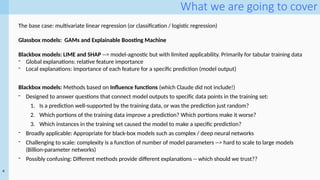
What we aregoing to cover
The base case: multivariate linear regression (or classification / logistic regression)
Glassbox models: GAMs and Explainable Boosting Machine
Blackbox models: LIME and SHAP --> model-agnostic but with limited applicability. Primarily for tabular training data
- Global explanations: relative feature importance
- Local explanations: importance of each feature for a specific prediction (model output)
Blackbox models: Methods based on Influence functions (which Claude did not include!)
- Designed to answer questions that connect model outputs to specific data points in the training set:
1. Is a prediction well-supported by the training data, or was the prediction just random?
2. Which portions of the training data improve a prediction? Which portions make it worse?
3. Which instances in the training set caused the model to make a specific prediction?
- Broadly applicable: Appropriate for black-box models such as complex / deep neural networks
- Challenging to scale: complexity is a function of number of model parameters --> hard to scale to large models
(Billion-parameter networks)
- Possibly confusing: Different methods provide different explanations -- which should we trust??
6
<event
name>
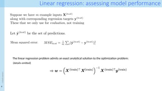
Linear regression: assessingmodel performance
The linear regression problem admits an exact analytical solution to the optimization problem:
(details omitted)
7.
7
<event
name>
GAM and ExplainableBoosting Machine
[1] Yin Lou, Rich Caruana, and Johannes Gehrke. 2012. Intelligible models for classification and regression. In Proceedings of the 18th ACM SIGKDD
international conference on Knowledge discovery and data mining (KDD '12). Association for Computing Machinery, New York, NY, USA, 150–158.
https://doi.org/10.1145/2339530.2339556
Goal: construct accurate models that are also interpretable
Interpretability: the model can quantify the impact of each predictor (feature)
- Locally: for a specific instance prediction
- Globally: over the entire set of predictions
Generalised Additive Models are linear models where the feature weights are themselves functions:
- The functions fi are not necessarily linear
- g() is the link function: logistic --> classification, identity --> regression etc
8.
8
<event
name>
Example (from [1])
Concretedataset: predict the compressive strength of concrete as a function of it age and ingredients
- Regression model
- 8 features. Including cement, water, age
the compressibility of concrete depends
nearly linearly on the Cement feature,
but it is a complex non-linear function of
the Water and Age features
Interpretability:
Accuracy: Each feature xi can have a complex non-linear shape fi(xi), and thus the accuracy of additive
models can be significantly higher than the accuracy of simple linear models.
9.
9
<event
name>
Spline-based GAMs –quick overview
First, we have to select
(i) the shape functions for individual features and
(ii) the learning method used to train the overall model
(i): [1] considers two types of shape functions:
Regression splines
✗ Trees and tree ensembles
Regression splines have the form: Where the bk are the basis functions and parameter
d is the degree of the spline
Further reading: https://bookdown.org/ssjackson300/Machine-Learning-Lecture-Notes/splines.html
Learning method:
Least square fitting
<-- not covered here
10.
10
<event
name>
From GAM toGA2
M
GA2
M: Generalized Additive Models plus Interactions
One limitation of GAM is that it cannot model interactions between features.
This limits its accuracy relative to full complexity models
Goal: extend GAMs to include pairwise interactions whilst maintaining interpretability
Two-dimensional interactions can still be rendered as heatmaps of fij(xi, xj) on the two-dimensional xi, xj-plane,
and thus a model that includes only one- and two-dimensional components is still intelligible. [3]
[3] Lou, Yin, Rich Caruana, Johannes Gehrke, and Giles Hooker. ‘Accurate Intelligible Models with Pairwise Interactions’. Proceedings of the 19th ACM
SIGKDD International Conference on Knowledge Discovery and Data Mining - KDD ’13, 2013, 623. https://doi.org/10.1145/2487575.2487579.
Challenge: for high-dimensional problems (N > 1000), testing all pairwise interactions is intractable
Approach: find an efficient statistics method to filter out all “irrelevant” interactions
FAST: an efficient method to measure and rank the strength of the interaction of all pairs of variables.
11.
11
<event
name>
Explainable Boosting Machinesand InterpretML
EBM is a fast implementation of GA2
M
It can learn generalized additive model (GAM) of the form:
[4a] Nori, Harsha, Samuel Jenkins, Paul Koch, and Rich Caruana. ‘InterpretML: A Unified Framework for Machine Learning Interpretability’, September
2019. http://arxiv.org/abs/1909.09223
[4b] Lou, Yin, Rich Caruana, Johannes Gehrke, and Giles Hooker. ‘Accurate Intelligible Models with Pairwise Interactions’. Proceedings of the 19th ACM
SIGKDD International Conference on Knowledge Discovery and Data Mining - KDD ’13, 2013, 623. https://doi.org/10.1145/2487575.2487579.
Learn the best feature function fj for each feature to show how each feature contributes to the model’s
prediction for the problem
- using bagging and gradient boosting
But it can also learn GA2
M models:
Exercise: experiment with the InterpretML python library:
https://github.com/interpretml/interpret
12.
12
<event
name>
Example: InterpretML inaction
[5] Caruana, Rich, Yin Lou, Johannes Gehrke, Paul Koch, Marc Sturm, and Noemie Elhadad. ‘Intelligible Models for Healthcare: Predicting Pneumonia Risk
and Hospital 30-Day Readmission’. In Proceedings of the 21th ACM SIGKDD International Conference on Knowledge Discovery and Data Mining, 1721–30.
ACM, 2015.
Case study: pneumonia datasets
- 14,199 pneumonia patients (70:30 train:test split)
- 46 features:
- age and gender, heart rate, blood pressure, and respiration rate
- lab tests such as White Blood Cell count (WBC) and Blood Urea Nitrogen (BUN)
- chest x-ray features: lung collapse or pleural effusion
Task: predict Probability Of Death (POD) so that patients at high risk can be admitted to the hospital, while
patients at low risk are treated as outpatients
- 10.86% of the patients in the dataset (1542 patients) died from pneumonia
13.
13
<event
name>
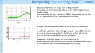
Interpreting by visualisingshape functions
Age (in years) on the x-axis ranges from 18-106 years old
The vertical axis is the risk score predicted by the model for patients as a
function of age
The risk score for this term varies from -0.25 for patients with age less than
50, to a high of about 0.35 for patients age 85 and above.
In reality, the explanation is that the aggressive care received by asthmatic
pneumonia patients was so effective that it lowered their risk of dying
from pneumonia compared to the general population.
This can be a misleading signal if not interpreted correctly:
models trained on the data incorrectly learn that asthma lowers risk, when
in fact asthmatics have much higher risk (if not hospitalized).
It appears that having asthma lowers the risk of dying from pneumonia
14.
14
<event
name>
Interpreting by visualisingshape functions
BUN is Blood Urea Nitrogen level
Most patients have BUN=0 because if they are assumed to be healthy, BUN is
not measured.
Thus you need to be careful when interpreting the chart, as “N/A” is not the
same as “value = 0”.
However one may speculate that “risk is reduced for patients where BUN was
not measured, because those are healthy patients”
When BUN is available:
- levels below 30 appear to be low risk
- levels from 50-200 indicate higher risk
This is consistent with medical knowledge which suggests that normal,
healthy BUN is 10-20, and that elevated levels above 30 may indicate kidney
damage, congestive heart failure, or bleeding in the gastrointestinal tract.
15.
15
<event
name>
Interpreting by visualisingshape functions
the model suggests that chronic lung disease and a history of chest pain both
decrease POD
Possible explanation: patients with lung disease and chest pain may receive care
earlier, and may receive more aggressive care
If this is verified, then both terms would be removed from the model
See the complete set of shape functions in the paper (Fig. 1): https://doi.org/10.1145/2783258.2788613
16.
16
<event
name>
Visualising pairwise interactions
Riskis highest for the youngest patients (probably cancers acquired in
childhood but not cured when the patient reaches age 18), and declines
for patients who acquire cancer later in life, but for patients without
cancer risk rises as expected with age
17.
17
<event
name>
Local Interpretable Model-agnosticExplanations (LIME)
[5] Ribeiro, Marco Tulio, Sameer Singh, and Carlos Guestrin. ‘Model-Agnostic Interpretability of Machine Learning’. In 2016 ICML Workshop on Human
Interpretability in Machine Network Learning (WHI 2016), 2016. https://doi.org/10.1145/2858036.2858529.
[6] Ribeiro, Marco Tulio, Singh, Sameer, and Guestrin, Carlos. “why should I trust you?”: Explaining the predictions of any classifier. In Knowledge
Discovery and Data Mining (KDD), 2016.
A model-agnostic method to generate local explanations
Main idea: for each instance vector generate an interpretable representation in a new space:
For instance: x may be a feature vector containing word embeddings, with x′ being the bag of words
LIME’s goal is to identify an interpretable model g over the interpretable representation that is locally faithful to the
classifier.
- The interpretable model may not be able to approximate the black box model globally
- However, approximating it in the vicinity of an individual instance may be feasible
The explanation consists of an interpretable model g (linear, decision trees, etc) that can be
presented to the user as the explanation for a specific instance:
18.
18
<event
name>
LIME
Model being explained:
Measureof proximity between an instance z to x: defines locality around x:
Measure of how ‘unfaithful’ g is in approximating f in the locality defined by
Measure of complexity (as opposed to interpretability) of g in a space of models G
- a soft constraint (e.g. the depth of a tree, or the number of non-zeros in a linear model)
- a hard constraint (e.g. ∞ if the depth or the number of non-zeros is above a certain
threshold).
LIME aims to ensure both interpretability and local fidelity
It aims to minimize while having low enough to be interpretable by humans
Approach: estimate by generating perturbed samples around x
making predictions with the black box model f and weighting them according to
20
<event
name>
Data Shapley: SHAP
[7]Ghorbani, Amirata, and James Zou. ‘Data Shapley: Equitable Valuation of Data for Machine Learning’. In Proceedings of the 36th International Conference
on Machine Learning, 2242–51. PMLR, 2019. https://proceedings.mlr.press/v97/ghorbani19c.html.
Given a training set and a learning algorithm, the aim is to
1) Identify an equitable measure of the value of each training data point to the learning algorithm with respect to some
performance metric
2) efficiently compute this data value in practical settings
Note: this is not a universal value for data. The value of each data point depends on:
- the learning algorithm
- the performance metric
- other data in the training set
This dependency is reasonable and desirable in machine learning. Certain data points could be more important if we are
training a logistic regression instead of a neural network.
21.
21
<event
name>
Baseline approach: Leave-one-out(LOO)
A simple idea to quantify the value of a single training data point:
compare the difference in the predictor’s performance when trained on the full dataset vs. the performance
when trained on the full set minus one point
Unfortunately, LOO does not satisfy natural properties for equitable data valuation, and it performs poorly in
experiments
Why does it fail?
- suppose we use a nearest-neighbor classifier: for each test point we find its nearest neighbor in the training set
and assign it that label
- suppose every training point has two exact copies in the training set
In this scenario, removing one point from training does not change the predictor at all, since its copy is still present.
LOO would simply assign value 0 to every data point
22.
22
<event
name>
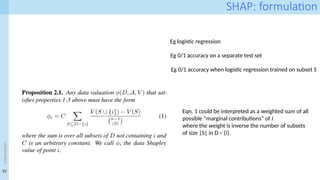
SHAP: formulation
Eg logisticregression
Eg 0/1 accuracy on a separate test set
Eg 0/1 accuracy when logistic regression trained on subset S
Eqn. 1 could be interpreted as a weighted sum of all
possible “marginal contributions” of I
where the weight is inverse the number of subsets
of size |S| in D − {i}.
23.
23
<event
name>
SHAP: Monte Carloapproximation
Computing data Shapley requires computing all the possible marginal contributions which is exponentially large in
the train data size
In addition, for each S D, computing V (S) involves learning a predictor on S using the learning algorithm A
⊆
1. sample a random permutations of data points
2. scan the permutation from the first element to
the last element and calculate the marginal
contribution of every new data point
3. Repeat the procedure over multiple Monte Carlo
permutations
The final estimation of the data Shapley is the average
of all the calculated marginal contributions
24.
24
<event
name>
Influence analysis
All modeldecisions are rooted in the training data [1]
Origins of the idea: Influence analysis (aka data valuation, data attribution) emerged alongside the initial study of
linear models and regression
- Focus on quantifying how worst-case perturbations to the training data affected the final model parameters
[1] Hammoudeh, Zayd, and Daniel Lowd. ‘Training Data Influence Analysis and Estimation: A Survey’. Machine Learning 113, no. 5 (1 May 2024): 2351–
2403. https://doi.org/10.1007/s10994-023-06495-7.
The idea of using Influence Functions to support black-box explanations originates around the same time as LIME
and SHAP, but uses a distinctly different approach
- aiming to trace a model's prediction through its learning algorithm and back to the training data
Complexity problem: determining a single training instance’s exact effect can be NP-complete in the worst case
Influence may not need to be measured exactly.
- Influence estimation methods provide an approximation of training instances’ true influence
- This is much more computationally efficient
- Influence estimators achieve their efficiency via various assumptions about the model’s architecture and learning
environment (Koh & Liang, 2017)
25.
25
<event
name>
General introduction
[1] Hammoudeh,Zayd, and Daniel Lowd. ‘Training Data Influence Analysis and Estimation: A Survey’. Machine Learning 113, no. 5 (1 May
2024): 2351–2403. https://doi.org/10.1007/s10994-023-06495-7
• Sec 2: General Notation
• Sec 3: Overview of influence and influence estimation
• 3.1 Pointwise training data influence
• Retraining-Based Methods
• Gradient-Based Influence Estimators
• Sec 5: Gradient based influence estimation
‑
• 5.1.1: influence functions
26.
26
<event
name>
Technical deep dive
[2]Koh, Pang Wei, and Percy Liang. ‘Understanding Black-Box Predictions via Influence Functions’. In Proceedings
of the 34th International Conference on Machine Learning, 1885–94. PMLR, 2017.
https://proceedings.mlr.press/v70/koh17a.html
The key idea is that IF makes it possible to observe changes in the model’s parameters as one single training point is
“upweighted” by an infinitesimal amount
In practice, this amounts to “differentiating through the training” to estimate, in closed form, the effect of training
perturbations
Intuitively, the idea is to estimate the change in the parameters Θ of the model due to removing a single
𝜃 ∈
point from the training set.
𝑧
Learning amounts to optimizing the parameters:
28
<event
name>
… now let’shead to the paper directly: https://proceedings.mlr.press/v70/koh17a.html
Exercise: experiment with the Infliuenciae python library: https://deel-ai.github.io/influenciae/
- Pick a dataset and learning task: Titanic + survive classifier
- Calculate influence for specific model inferences
- Comment on the observed most influential data points
29.
29
<event
name>
Tracin
[3] Pruthi, Garima,Frederick Liu, Satyen Kale, and Mukund Sundararajan. ‘Estimating Training Data Influence by Tracing
Gradient Descent’. In Advances in Neural Information Processing Systems, 33:19920–30. Curran Associates, Inc., 2020.
https://proceedings.neurips.cc/paper_files/paper/2020/hash/e6385d39ec9394f2f3a354d9d2b88eec-Abstract.html
Let’s head directly to the paper:
Exercise: experiment with the Tracin python library:
https://colab.research.google.com/drive/1E94cGF46SUQXcCTNwQ4VGSjXEKm7g21c?usp=sharing
- Pick a dataset and learning task: Titanic + survive yes/no classifier
- Calculate influence for specific model inferences
- Comment on the observed most influential data points
Focus on
- Sec. 3.1: Idealized Notion of Influence
- Sec 3.2: First-order Approximation to Idealized Influence
30.
30
<event
name>
Additional reading materialon XAI
Hu, Yuzheng, Pingbang Hu, Han Zhao, and Jiaqi W. Ma. ‘Most Influential Subset Selection: Challenges, Promises, and Beyond’. arXiv, 8
January 2025. https://doi.org/10.48550/arXiv.2409.18153.
Guo, Han, Nazneen Fatema Rajani, Peter Hase, Mohit Bansal, and Caiming Xiong. ‘FastIF: Scalable Influence Functions for Efficient Model
Interpretation and Debugging’. arXiv, 9 September 2021. https://doi.org/10.48550/arXiv.2012.15781.
Brophy, Jonathan, Zayd Hammoudeh, and Daniel Lowd. "Adapting and evaluating influence-estimation methods for gradient-boosted
decision trees." Journal of Machine Learning Research 24.154 (2023): 1-48.
Basu, Samyadeep, Philip Pope, and Soheil Feizi. ‘Influence Functions in Deep Learning Are Fragile’. arXiv, 10 February 2021.
https://doi.org/10.48550/arXiv.2006.14651.
Bae, Juhan, Nathan Ng, Alston Lo, Marzyeh Ghassemi, and Roger Grosse. ‘If Influence Functions Are the Answer, Then What Is the
Question?’ arXiv, 12 September 2022. https://doi.org/10.48550/arXiv.2209.05364.
M. Sahakyan, Z. Aung and T. Rahwan, "Explainable Artificial Intelligence for Tabular Data: A Survey," in IEEE Access, vol. 9, pp. 135392-
135422, 2021, doi: 10.1109/ACCESS.2021.3116481.
Borisov, Vadim, et al. "Deep neural networks and tabular data: A survey." IEEE transactions on neural networks and learning
systems (2022).
Ren, Weijieying, et al. "Deep Learning within Tabular Data: Foundations, Challenges, Advances and Future Directions." arXiv preprint
arXiv:2501.03540 (2025).
Jacob R. Epifano, Ravi P. Ramachandran, Aaron J. Masino, Ghulam Rasool, Revisiting the fragility of influence functions, Neural Networks,
Volume 162, 2023, Pages 581-588, ISSN 0893-6080, https://doi.org/10.1016/j.neunet.2023.03.029.
Editor's Notes
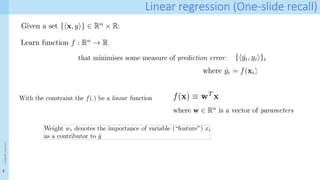
#5 Given a set $\{\langle \mathbf{x}, y \rangle \} \in \mathbb{R}^n \times \mathbb{R}$:
Learn function $f: \mathbb{R}^n \rightarrow \mathbb{R}$
that minimises some measure of \textit{prediction error}:
$ \{ \langle \hat{y_i}, y_i \rangle \}_i $
where $\hat{y_i} = f(\mathbf{x}_i)$
With the constraint the $f(.)$ be a \textit{linear} function
#6 \noindent Suppose we have $m$ example inputs $\mathbf{X}^{(test()$ \\
along with corresponding regression targets $\mathbf{y}^{(test)}$\\
These that we only use for \textit{evaluation}, not training
Let $ \hat{\mathbf{y}}^{(test)}$ be the set of predictions.
Mean squared error:
1 - \frac{\sum_{i:1}^{n}(y_i - \hat{y}_i)^2}{\sum_{i:1}^{n}(y_i - \bar{y})^2}


![7
<event
name>
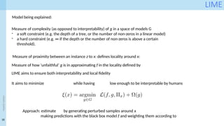
GAM and Explainable Boosting Machine
[1] Yin Lou, Rich Caruana, and Johannes Gehrke. 2012. Intelligible models for classification and regression. In Proceedings of the 18th ACM SIGKDD
international conference on Knowledge discovery and data mining (KDD '12). Association for Computing Machinery, New York, NY, USA, 150–158.
https://doi.org/10.1145/2339530.2339556
Goal: construct accurate models that are also interpretable
Interpretability: the model can quantify the impact of each predictor (feature)
- Locally: for a specific instance prediction
- Globally: over the entire set of predictions
Generalised Additive Models are linear models where the feature weights are themselves functions:
- The functions fi are not necessarily linear
- g() is the link function: logistic --> classification, identity --> regression etc](https://image.slidesharecdn.com/xai-05-25pm-250520042913-2123cb9b/85/A-simple-Introduction-to-Explainability-in-Machine-Learning-and-AI-XAI-7-320.jpg)
![8
<event
name>
Example (from [1])
Concrete dataset: predict the compressive strength of concrete as a function of it age and ingredients
- Regression model
- 8 features. Including cement, water, age
the compressibility of concrete depends
nearly linearly on the Cement feature,
but it is a complex non-linear function of
the Water and Age features
Interpretability:
Accuracy: Each feature xi can have a complex non-linear shape fi(xi), and thus the accuracy of additive
models can be significantly higher than the accuracy of simple linear models.](https://image.slidesharecdn.com/xai-05-25pm-250520042913-2123cb9b/85/A-simple-Introduction-to-Explainability-in-Machine-Learning-and-AI-XAI-8-320.jpg)
![9
<event
name>
Spline-based GAMs – quick overview
First, we have to select
(i) the shape functions for individual features and
(ii) the learning method used to train the overall model
(i): [1] considers two types of shape functions:
Regression splines
✗ Trees and tree ensembles
Regression splines have the form: Where the bk are the basis functions and parameter
d is the degree of the spline
Further reading: https://bookdown.org/ssjackson300/Machine-Learning-Lecture-Notes/splines.html
Learning method:
Least square fitting
<-- not covered here](https://image.slidesharecdn.com/xai-05-25pm-250520042913-2123cb9b/85/A-simple-Introduction-to-Explainability-in-Machine-Learning-and-AI-XAI-9-320.jpg)
![10
<event
name>
From GAM to GA2
M
GA2
M: Generalized Additive Models plus Interactions
One limitation of GAM is that it cannot model interactions between features.
This limits its accuracy relative to full complexity models
Goal: extend GAMs to include pairwise interactions whilst maintaining interpretability
Two-dimensional interactions can still be rendered as heatmaps of fij(xi, xj) on the two-dimensional xi, xj-plane,
and thus a model that includes only one- and two-dimensional components is still intelligible. [3]
[3] Lou, Yin, Rich Caruana, Johannes Gehrke, and Giles Hooker. ‘Accurate Intelligible Models with Pairwise Interactions’. Proceedings of the 19th ACM
SIGKDD International Conference on Knowledge Discovery and Data Mining - KDD ’13, 2013, 623. https://doi.org/10.1145/2487575.2487579.
Challenge: for high-dimensional problems (N > 1000), testing all pairwise interactions is intractable
Approach: find an efficient statistics method to filter out all “irrelevant” interactions
FAST: an efficient method to measure and rank the strength of the interaction of all pairs of variables.](https://image.slidesharecdn.com/xai-05-25pm-250520042913-2123cb9b/85/A-simple-Introduction-to-Explainability-in-Machine-Learning-and-AI-XAI-10-320.jpg)
![11
<event
name>
Explainable Boosting Machines and InterpretML
EBM is a fast implementation of GA2
M
It can learn generalized additive model (GAM) of the form:
[4a] Nori, Harsha, Samuel Jenkins, Paul Koch, and Rich Caruana. ‘InterpretML: A Unified Framework for Machine Learning Interpretability’, September
2019. http://arxiv.org/abs/1909.09223
[4b] Lou, Yin, Rich Caruana, Johannes Gehrke, and Giles Hooker. ‘Accurate Intelligible Models with Pairwise Interactions’. Proceedings of the 19th ACM
SIGKDD International Conference on Knowledge Discovery and Data Mining - KDD ’13, 2013, 623. https://doi.org/10.1145/2487575.2487579.
Learn the best feature function fj for each feature to show how each feature contributes to the model’s
prediction for the problem
- using bagging and gradient boosting
But it can also learn GA2
M models:
Exercise: experiment with the InterpretML python library:
https://github.com/interpretml/interpret](https://image.slidesharecdn.com/xai-05-25pm-250520042913-2123cb9b/85/A-simple-Introduction-to-Explainability-in-Machine-Learning-and-AI-XAI-11-320.jpg)
![12
<event
name>
Example: InterpretML in action
[5] Caruana, Rich, Yin Lou, Johannes Gehrke, Paul Koch, Marc Sturm, and Noemie Elhadad. ‘Intelligible Models for Healthcare: Predicting Pneumonia Risk
and Hospital 30-Day Readmission’. In Proceedings of the 21th ACM SIGKDD International Conference on Knowledge Discovery and Data Mining, 1721–30.
ACM, 2015.
Case study: pneumonia datasets
- 14,199 pneumonia patients (70:30 train:test split)
- 46 features:
- age and gender, heart rate, blood pressure, and respiration rate
- lab tests such as White Blood Cell count (WBC) and Blood Urea Nitrogen (BUN)
- chest x-ray features: lung collapse or pleural effusion
Task: predict Probability Of Death (POD) so that patients at high risk can be admitted to the hospital, while
patients at low risk are treated as outpatients
- 10.86% of the patients in the dataset (1542 patients) died from pneumonia](https://image.slidesharecdn.com/xai-05-25pm-250520042913-2123cb9b/85/A-simple-Introduction-to-Explainability-in-Machine-Learning-and-AI-XAI-12-320.jpg)


![17
<event
name>
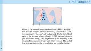
Local Interpretable Model-agnostic Explanations (LIME)
[5] Ribeiro, Marco Tulio, Sameer Singh, and Carlos Guestrin. ‘Model-Agnostic Interpretability of Machine Learning’. In 2016 ICML Workshop on Human
Interpretability in Machine Network Learning (WHI 2016), 2016. https://doi.org/10.1145/2858036.2858529.
[6] Ribeiro, Marco Tulio, Singh, Sameer, and Guestrin, Carlos. “why should I trust you?”: Explaining the predictions of any classifier. In Knowledge
Discovery and Data Mining (KDD), 2016.
A model-agnostic method to generate local explanations
Main idea: for each instance vector generate an interpretable representation in a new space:
For instance: x may be a feature vector containing word embeddings, with x′ being the bag of words
LIME’s goal is to identify an interpretable model g over the interpretable representation that is locally faithful to the
classifier.
- The interpretable model may not be able to approximate the black box model globally
- However, approximating it in the vicinity of an individual instance may be feasible
The explanation consists of an interpretable model g (linear, decision trees, etc) that can be
presented to the user as the explanation for a specific instance:](https://image.slidesharecdn.com/xai-05-25pm-250520042913-2123cb9b/85/A-simple-Introduction-to-Explainability-in-Machine-Learning-and-AI-XAI-17-320.jpg)
![20
<event
name>
Data Shapley: SHAP
[7] Ghorbani, Amirata, and James Zou. ‘Data Shapley: Equitable Valuation of Data for Machine Learning’. In Proceedings of the 36th International Conference
on Machine Learning, 2242–51. PMLR, 2019. https://proceedings.mlr.press/v97/ghorbani19c.html.
Given a training set and a learning algorithm, the aim is to
1) Identify an equitable measure of the value of each training data point to the learning algorithm with respect to some
performance metric
2) efficiently compute this data value in practical settings
Note: this is not a universal value for data. The value of each data point depends on:
- the learning algorithm
- the performance metric
- other data in the training set
This dependency is reasonable and desirable in machine learning. Certain data points could be more important if we are
training a logistic regression instead of a neural network.](https://image.slidesharecdn.com/xai-05-25pm-250520042913-2123cb9b/85/A-simple-Introduction-to-Explainability-in-Machine-Learning-and-AI-XAI-20-320.jpg)

![24
<event
name>
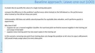
Influence analysis
All model decisions are rooted in the training data [1]
Origins of the idea: Influence analysis (aka data valuation, data attribution) emerged alongside the initial study of
linear models and regression
- Focus on quantifying how worst-case perturbations to the training data affected the final model parameters
[1] Hammoudeh, Zayd, and Daniel Lowd. ‘Training Data Influence Analysis and Estimation: A Survey’. Machine Learning 113, no. 5 (1 May 2024): 2351–
2403. https://doi.org/10.1007/s10994-023-06495-7.
The idea of using Influence Functions to support black-box explanations originates around the same time as LIME
and SHAP, but uses a distinctly different approach
- aiming to trace a model's prediction through its learning algorithm and back to the training data
Complexity problem: determining a single training instance’s exact effect can be NP-complete in the worst case
Influence may not need to be measured exactly.
- Influence estimation methods provide an approximation of training instances’ true influence
- This is much more computationally efficient
- Influence estimators achieve their efficiency via various assumptions about the model’s architecture and learning
environment (Koh & Liang, 2017)](https://image.slidesharecdn.com/xai-05-25pm-250520042913-2123cb9b/85/A-simple-Introduction-to-Explainability-in-Machine-Learning-and-AI-XAI-24-320.jpg)
![25
<event
name>
General introduction
[1] Hammoudeh, Zayd, and Daniel Lowd. ‘Training Data Influence Analysis and Estimation: A Survey’. Machine Learning 113, no. 5 (1 May
2024): 2351–2403. https://doi.org/10.1007/s10994-023-06495-7
• Sec 2: General Notation
• Sec 3: Overview of influence and influence estimation
• 3.1 Pointwise training data influence
• Retraining-Based Methods
• Gradient-Based Influence Estimators
• Sec 5: Gradient based influence estimation
‑
• 5.1.1: influence functions](https://image.slidesharecdn.com/xai-05-25pm-250520042913-2123cb9b/85/A-simple-Introduction-to-Explainability-in-Machine-Learning-and-AI-XAI-25-320.jpg)
![26
<event
name>
Technical deep dive
[2] Koh, Pang Wei, and Percy Liang. ‘Understanding Black-Box Predictions via Influence Functions’. In Proceedings
of the 34th International Conference on Machine Learning, 1885–94. PMLR, 2017.
https://proceedings.mlr.press/v70/koh17a.html
The key idea is that IF makes it possible to observe changes in the model’s parameters as one single training point is
“upweighted” by an infinitesimal amount
In practice, this amounts to “differentiating through the training” to estimate, in closed form, the effect of training
perturbations
Intuitively, the idea is to estimate the change in the parameters Θ of the model due to removing a single
𝜃 ∈
point from the training set.
𝑧
Learning amounts to optimizing the parameters:](https://image.slidesharecdn.com/xai-05-25pm-250520042913-2123cb9b/85/A-simple-Introduction-to-Explainability-in-Machine-Learning-and-AI-XAI-26-320.jpg)

![29
<event
name>
Tracin
[3] Pruthi, Garima, Frederick Liu, Satyen Kale, and Mukund Sundararajan. ‘Estimating Training Data Influence by Tracing
Gradient Descent’. In Advances in Neural Information Processing Systems, 33:19920–30. Curran Associates, Inc., 2020.
https://proceedings.neurips.cc/paper_files/paper/2020/hash/e6385d39ec9394f2f3a354d9d2b88eec-Abstract.html
Let’s head directly to the paper:
Exercise: experiment with the Tracin python library:
https://colab.research.google.com/drive/1E94cGF46SUQXcCTNwQ4VGSjXEKm7g21c?usp=sharing
- Pick a dataset and learning task: Titanic + survive yes/no classifier
- Calculate influence for specific model inferences
- Comment on the observed most influential data points
Focus on
- Sec. 3.1: Idealized Notion of Influence
- Sec 3.2: First-order Approximation to Idealized Influence](https://image.slidesharecdn.com/xai-05-25pm-250520042913-2123cb9b/85/A-simple-Introduction-to-Explainability-in-Machine-Learning-and-AI-XAI-29-320.jpg)