Developing an effective AI/ML model risk management program, with topics covering - Understanding machine learning lifecycle in banking - Understanding key elements of machine learning model validation - Testing modules for conceptual soundness - Testing modules for outcome analysis - Developing inherently interpretable benchmark models - Developing the automated pipeline for streamlined validation - Enabling automated validation and monitoring for dynamically updating models

1. Machine Learning Model Validation
Developing an effective AI/ML model risk management program
Aijun Zhang
SVP, Head of Validation Engineering
Corporate Model Risk, Wells Fargo
CeFPro 3rd Annual Advanced Model Risk Conference | March 12-13, 2024 | NYC
Disclaimer: This material represents the views of the presenter and does not necessarily reflect those of Wells Fargo.

2. Machine Learning Lifecycle
Data
Collection, Labelling,
Loading, Preprocessing,
Quality Check,
Data Visualization,
Feature Engineering,
Variable Selection
Model Development
Model Design and Assumptions,
Model Training,
Hyperparameter Tuning,
Model Calibration,
Developmental Testing,
Developmental Benchmarking
Model Validation
Independent Testing,
Independent Benchmarking,
Data Quality Check,
Conceptual Soundness,
Outcome Analysis
Plan Data Development Validation Deployment Monitoring Retire
Use
Model Change/Dynamic Update

3. Machine Learning Model Validation - Key Elements
Weakness
• Segmented metrics
• Weak region detection
• Overfitting region detection
Data Quality
•
Data integrity check
•
Outlier detection
•
Distribution drift analysis
Model
Explainability
•
Feature importance
•
Partial dependence
•
Local explainability
Interpretable
Benchmarking
•
Interpretable models
•
Benchmark performance
•
Benchmark interpretability
Variable
Selection
•
Correlation analysis
•
Surrogated importance
•
Conditional independence
Reliability
• Prediction Uncertainty
• Reliability diagram
• Conformal prediction
Robustness
• Input noise perturbation
• Performance degradation
• Benchmarking analysis
Resilience
• Distribution drift
• Resilient scenarios
• Sensitive feature detection
Conceptual Soundness Outcome Analysis

4. PiML Toolbox Overview
Model Development
• Data Exploration and Quality Check
• Inherently Interpretable ML Models
– GLM, GAM, XGB1
– XGB2, EBM, GAMI-Net, GAMI-Lin-Tree
• Locally Interpretable ML Models
– Tree, Sparse ReLU Neural Networks
• Model-specific Interpretability
• Model-agnostic Explainability
Model Testing
• Model Diagnostics and Outcome Analysis
– Prediction Accuracy
– Hyperparameter Turning
– Weakness Detection
– Reliability Test (Prediction Uncertainty)
– Robustness Test
– Resilience Test
– Bias and Fairness
• Model Comparison and Benchmarking
4
An integrated Python toolbox for interpretable machine learning

5. Explainability Test
• Post-hoc explainability test is model-agnostic, i.e., it works for any pre-trained model.
– Useful for explaining black-box models; but need to use with caution (there is no free lunch).
– Post-hoc explainability tools sometimes have pitfalls, challenges and potential risks.
• Local explainability tools for explaining an individual prediction
– ICE (Individual Conditional Expectation) plot
– LIME (Local Interpretable Model-agnostic Explanations)
– SHAP (SHapley Additive exPlanations)
• Global explainability tools for explaining the overall impact of features on model predictions
– Examine relative importance of variables: VI (Variable Importance), PFI (Permutation Feature Importance), SHAP-FI
(SHAP Feature Importance), H-statistic (Importance of two-factor interactions), etc.
– Understand input-output relationships: 1D and 2D PDP (Partial Dependence Plot) and ALE (Accumulated Local Effects).
5

6. Post-hoc Explainability vs. Inherent Interpretability
• Post-hoc explainability is model agnostic, but there is
no free lunch. According to Cynthia Rudin, use of
auxiliary post-hoc explainers creates “double trouble”
for black-box models.
• Various post-hoc explanation methods, including VI/FI,
PDP, ALE, … (for global explainability) and LIME, SHAP,
… (for local explainability), often produce results with
disagreements.
• Lots of academic discussions about pitfalls, challenges
and potential risks of using post-hoc explainers.
• This echoes CFPB Circular 2022-03 (May 26, 2022):
Adverse action notification requirements in connection
with credit decisions based on complex algorithms1.
• Inherent interpretability is intrinsic to a model. It
facilitates gist and intuitiveness for human insightful
interpretation. It is important for evaluating a model’s
conceptual soundness.
• Model interpretability is a loosely defined concept and
can be hardly quantified. Sudjianto and Zhang (2021)2
proposed a qualitative rating assessment framework
for ML model interpretability.
• Interpretable model design: a) interpretable feature
selection and b) interpretable architecture constraints3
such as additivity, sparsity, linearity, smoothness,
monotonicity, visualizability, projection orthogonality,
and segmentation degree.
1 CFPB Circular 2022-03 Footnote 1: “While some creditors may rely upon various post-hoc explanation methods, such explanations approximate models and
creditors must still be able to validate the accuracy of those approximations, which may not be possible with less interpretable models.” consumerfinance.gov
2 Sudjianto and Zhang (2021): Designing Inherently Interpretable Machine Learning Models. arXiv: 2111.01743
3 Yang, Zhang and Sudjianto (2021, IEEE TNNLS): Enhancing Explainability of Neural Networks through Architecture Constraints. arXiv: 1901.03838
6

7. Inherently Interpretable FANOVA Models
• One effective way is to design inherently interpretable models by the functional ANOVA representation
𝑔 𝔼 𝑦 𝒙 = 𝑔0 + ෍
𝑗
𝑔𝑗 𝑥𝑗 + ෍
𝑗<𝑘
𝑔𝑗𝑘 𝑥𝑗, 𝑥𝑘 + ෍
𝑗<𝑘<𝑙
𝑔𝑗𝑘𝑙 𝑥𝑗, 𝑥𝑘, 𝑥𝑙 + ⋯
It additively decomposes into the overall mean (i.e., intercept) 𝑔0, main effects 𝑔𝑗 𝑥𝑗 , two-factor interactions
𝑔𝑗𝑘 𝑥𝑗, 𝑥𝑘 , and higher-order interactions …
• GAM main-effect models: Binning Logistic, XGB1, GAM (estimated using Splines, etc.)
• GAMI main-effect plus two-factor-interaction models:
– EBM (Nori, et al. 2019) → explainable boosting machine with shallow trees
– XGB2 (Lengerich, et al. 2020) → boosted trees of depth 2 with effect purification
– GAMI-Net(Yang, Zhang and Sudjianto, 2021) → specialized neural nets
– GAMI-Lin-Tree (Hu, et al. 2023) → specialized boosted linear model-based trees
• PiML Toolbox integrates GLM, GAM, XGB1, XGB2, EBM, GAMI-Net and GAMI-Lin-Tree, and provides each
model’s inherent interpretability.
7

8. XGB1, XGB2 and Beyond
• Proposition: A depth-𝐾 tree-ensemble can be reformulated to an FANOVA model with main effects and 𝑘-
way interactions with 𝑘 ≤ 𝐾.
• Examples: XGB1 is GAM with main effects; XGB2 is GAMI with main effects plus two-factor interactions.
• Three-step unwrapping technique for tree ensembles (e.g., RF, GBDT, XGBoost, LightGBM, CatBoost):
1. Aggregation: all leaf nodes with the same set of 𝑘 distinct split variables sum up to a raw 𝑘-way interaction.
2. Purification: recursively cascade effects from high-order interactions to lower-order ones to obtain a unique FANOVA
representation subject to hierarchical orthogonality constraints (Lengerich, et al., 2020).
3. Attribution: quantify the importance of purified effects either locally (for a sample) or globally (for a dataset).
• Strategies to enhance model (e.g., XGBoost) interpretability without sacrificing model performance
– XGB hyperparameters: max_tree_depth, max_bins, candidate interactions, monotonicity, L1/L2 regularization, etc.
– Pruning of purified effects: effect selection by L1 regularization, forward and backward selection with early stopping
– Other strategies such as post-hoc smoothing of purified effects, local flattening, and boundary effect adjustment.
8

9. EBM, GAMI-Lin-Tree, GAMI-Net
9
𝐆𝐀𝐌𝐈: 𝑔 𝐸 𝑦 𝒙 = 𝜇 + ෍ ℎ𝑗 𝑥𝑗 + ෍ 𝑓𝑗𝑘(𝑥𝑗, 𝑥𝑘)
EBM (Nori, et al. 2019)
GAMI-Lin-Tree (Hu, et al. 2023)

10. Deep ReLU Neural Networks
• Proposition: A ReLU DNN performs recursive oblique partitioning of the input domain into disjoint convex
regions. It predicts each region by a local linear model. See the Aletheia paper Sudjianto, et al. (2020)
• Just like decision tree, ReLU DNN enjoys exact local interpretability.
• Deep learning models often are overparametrized and less robust than simple models. PiML team has
proposed different ways to simplify DNNs and promotes L1-sparsification in the PiML toolbox.
10

11. Weakness Detection by Error Slicing
11
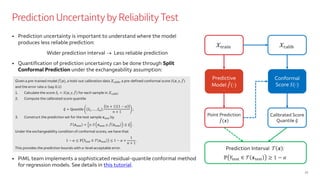
1. Specify an appropriate metric based on individual prediction residuals:
e.g., MSE for regression, ACC/AUC for classification, train-test
performance gap (for checking overfit), prediction interval bandwidth, ...
2. Specify 1 or 2 slicing features of interest;
3. Evaluate the metric for each sample in the target data (training or testing)
as pseudo responses;
4. Segment the target data along the slicing features, by
a) [Unsupervised] Histogram slicing with equal-space binning, or
b) [Supervised] fitting a decision tree to generate the sub-regions
5. Identify the sub-regions with average metric exceeding the pre-specified
threshold, subject to minimum sample condition.

12. Prediction Uncertainty by Reliability Test
12
• Prediction uncertainty is important to understand where the model
produces less reliable prediction:
Wider prediction interval → Less reliable prediction
• Quantification of prediction uncertainty can be done through Split
Conformal Prediction under the exchangeability assumption:
• PiML team implements a sophisticated residual-quantile conformal method
for regression models. See details in this tutorial.
Predictive
Model መ
𝑓(∙)
𝒳train
Point Prediction
መ
𝑓(𝒙)
𝒳calib
Prediction Interval 𝒯 𝒙 :
ℙ 𝑌test ∈ 𝒯 𝒙test ≥ 1 − 𝛼
Calibrated Score
Quantile ො
𝑞
Conformal
Score 𝑆(∙)
Given a pre-trained model መ
𝑓(𝒙), a hold-out calibration data 𝒳calib, a pre-defined conformal score 𝑆(𝒙, 𝑦, መ
𝑓)
and the error rate 𝛼 (say 0.1)
1. Calculate the score 𝑆𝑖 = 𝑆(𝒙, 𝑦, መ
𝑓) for each sample in 𝒳calib;
2. Compute the calibrated score quantile
ො
𝑞 = Quantile 𝑆1, … , 𝑆𝑛 ;
𝑛 + 1 1 − 𝛼
𝑛 + 1
;
3. Construct the prediction set for the test sample 𝒙test by
𝒯 𝒙test = 𝑦: 𝑆 𝒙test, 𝑦, መ
𝑓 𝒙test ≤ ො
𝑞 .
Under the exchangeability condition of conformal scores, we have that
1 − 𝛼 ≤ ℙ 𝑌test ∈ 𝒯 𝒙test ≤ 1 − 𝛼 +
1
𝑛 + 1
.
This provides the prediction bounds with α-level acceptable error.

13. Robustness and Resilience Tests
• Train-test data split (i.i.d.) leads to over-optimism of model performance,
since model in production will be exposed to data distribution shift.
• Robustness test: evaluate the performance degradation under covariate
noise perturbation:
– Perturb testing data covariates with small random noise;
– Assess model performance of perturbed testing data.
– Overfitting models often perform poorly in changing environments.
• Resilience test: evaluate the performance degradation under distribution
drift scenarios
– Scenarios: worst-sample, worst-cluster, outer-sample, hard-sample
– Measure distribution drift (e.g., PSI) of variables between worst performing
sample and the remaining sample.
– Variables with notable drift are deemed to be sensitive in the resilience test.
13
Model
Input Output
Shift
Happens
Environment
(Noise)
Error
Unintended outcome

14. Streamlined Validation of AI/ML Models
• Developing an effective AI/ML model risk management program: VoD (Validation-on-Demand) platform
• Key objective: streamline validation process to reduce cycle time and enable automated validation/
monitoring for AI/ML models (including dynamically updating models).
• Standard model wrapping - provides a standardized model management protocol for managing data and
model complexity and diversity.
• Standard validation tests - centralizes test codes and validation suites for data quality check, evaluation of
conceptual soundness, and outcome analysis.
Model Developer
• Developmental testing
• Wrap data and model
• Run validation suite
prescribed by validator
Model Validator
• Effective challenge
• Standard test codes
• Parameterize tests and
form validation suite
ValOps Platform
Automate routine
validation operations with
centralized tests and
distributed execution

15. Thank you
Aijun Zhang, Ph.D.
Email: Aijun.Zhang@wellsfargo.com
LinkedIn: https://www.linkedin.com/in/ajzhang/