Algorithmic bias and its effect on Machine Learning models. Simple fairness metrics and how to achieve them by fixing either the data, the model, or both

1. Prof. Paolo Missier
School of Computer Science
University of Birmingham, UK
Current Topics in Data Science
2024/25 Sem 2
Introduction to Algorithmic Fairness
Refs:
[1] Caton, Simon, and Christian Haas. ‘Fairness in Machine Learning: A Survey’. ACM Computing Surveys 56, no. 7 (31 July 2024): 1–38.
https://doi.org/10.1145/3616865

2. 2
<event
name>
Equality vs Equity vs removing barriers

3. 3
<event
name>
Algorithmic bias and protected attributes
Algorithmic bias refers to systematic errors in algorithmic decisions that create unfair outcomes
relative to certain protected attributes (or characteristics)
Protected attributes are those that contain information about ourselves that we generally
consider sensitive / private / confidential.
In the UK those are clearly identified in the UK Equality Act 2010:
• Age
• Disability
• Gender reassignment
• Marriage and civil partnership
• Pregnancy and maternity
• Race (including color, nationality, ethnic or national origin)
• Religion or belief
• Sex
• Sexual orientation

4. 4
<event
name>
A simple Machine Learning setting
To fix ideas and make things concrete, throughout this overview we are going
to consider a simple supervised Machine Learning setting:

5. 5
<event
name>
Algorithmic bias--> data bias
The bias (“unfairness”) observed in the model reflects bias in the data used to train the model
Thus we begin by understanding data bias, and then move on to model bias.
A high level classification for biased Training Data:
- Historical prejudice: observed when training
data contains historical human biases (e.g.,
past discriminatory lending practices)
- Representation disparities: When certain
demographic groups are underrepresented in
the data
Ex.: loans approved based on ethnicity
regardless of income
(bias: some groups are lower risk than
others)
Ex.: model rejects female candidates
based on sex because most positive
females are under-represented in training
set

6. 6
<event
name>
Proxy variables
Ex.: Suppose information about where someone has studied is available.
This “university faculty” variable is a proxy.
This may suggest (with some probability):
- the subject studied by an individual, which may correlate with gender
- the level of their education, itself a sensitive variable
If the model discriminates based on this variable, it is unfair although no sensitive variable is
used explicitly
Suppose we decide to remove the sensitive attributes from the data.
This will give “fairness by blinding”: there are simply no sensitive groups!
However, some variables may act as proxy for sensitive attributes

7. 7
<event
name>
Examples of proxy variables
Source: [1]

8. 8
<event
name>
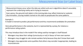
Measurement bias (or Label bias)
Measurement biases occur when the data we collect and use in algorithms doesn't accurately
represent the underlying reality we're trying to measure.
Even worse, the ground truth labels in the training data may reflect historical or systemic
discrimination, causing models trained on this data to perpetuate the same patterns
Example 1:
A model is trained to predict job performance and thus recommend candidates for promotion
Here job performance is the outcome, but it is represented by a proxy, for instance a
performance rating system.
This may introduce bias in the model if the rating used by managers is itself biased:
- Managers may skew their ratings (consciously or not) in favour of men over women
- Managers may struggle to rate remote workers fairly because they don’t know them well
- Managers may appreciate some qualities that others may consider inappropriate, leading to
inconsistencies

9. 9
<event
name>
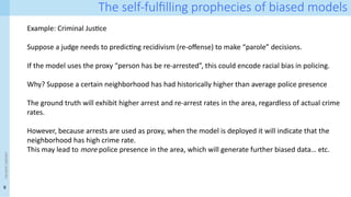
The self-fulfilling prophecies of biased models
Example: Criminal Justice
Suppose a judge needs to predicting recidivism (re-offense) to make “parole” decisions.
If the model uses the proxy “person has be re-arrested”, this could encode racial bias in policing.
Why? Suppose a certain neighborhood has had historically higher than average police presence
The ground truth will exhibit higher arrest and re-arrest rates in the area, regardless of actual crime
rates.
However, because arrests are used as proxy, when the model is deployed it will indicate that the
neighborhood has high crime rate.
This may lead to more police presence in the area, which will generate further biased data… etc.

10. 10
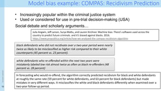
Model bias example: COMPAS: Recidivism Prediction
<event
name>
• Increasingly popular within the criminal justice system
• Used or considered for use in pre-trial decision-making (USA)
Social debate and scholarly arguments…
Julia Angwin, Jeff Larson, Surya Mattu, and Lauren Kirchner. Machine bias: There’s software used across the
country to predict future criminals. and it’s biased against blacks. 2016.
https://www.propublica.org/article/how-we-analyzed-the-compas-recidivism-algorithm
black defendants who did not recidivate over a two-year period were nearly
twice as likely to be misclassified as higher risk compared to their white
counterparts (45 percent vs. 23 percent).
white defendants who re-offended within the next two years were
mistakenly labeled low risk almost twice as often as black re-offenders (48
percent vs. 28 percent)
In forecasting who would re-offend, the algorithm correctly predicted recidivism for black and white defendants
at roughly the same rate (59 percent for white defendants, and 63 percent for black defendants) but made
mistakes in very different ways. It misclassifies the white and black defendants differently when examined over a
two-year follow-up period.

11. 11
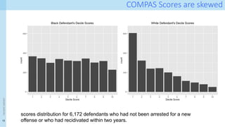
COMPAS Scores are skewed
<event
name>
scores distribution for 6,172 defendants who had not been arrested for a new
offense or who had recidivated within two years.

12. 12
<event
name>
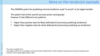
More on the recidivism example
The study is available here:
Julia Angwin, Jeff Larson, Surya Mattu, and Lauren Kirchner. Machine bias: There’s software used across the country to predict future
criminals. and it’s biased against blacks. 2016.
The COMPAS system for predicting criminal recidivism used "re-arrest" as its target variable.
The system had similar overall accuracy across racial groups
however it had different error patterns:
• Higher false positive rates for Black defendants (incorrectly predicting recidivism)
• Higher false negative rates for white defendants (incorrectly predicting no recidivism)

13. 13
<event
name>
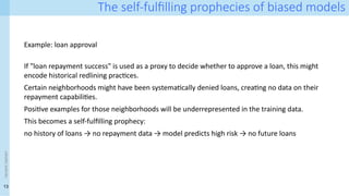
The self-fulfilling prophecies of biased models
Example: loan approval
If "loan repayment success" is used as a proxy to decide whether to approve a loan, this might
encode historical redlining practices.
Certain neighborhoods might have been systematically denied loans, creating no data on their
repayment capabilities.
Positive examples for those neighborhoods will be underrepresented in the training data.
This becomes a self-fulfilling prophecy:
no history of loans → no repayment data → model predicts high risk → no future loans

14. 14
<event
name>
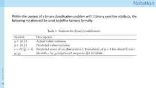
Notation
Within the context of a binary classification problem with 1 binary sensitive attribute, the
following notation will be used to define fairness formally:

15. 15
<event
name>
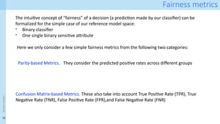
Fairness metrics
The intuitive concept of “fairness” of a decision (a prediction made by our classifier) can be
formalized for the simple case of our reference model space:
- Binary classifier
- One single binary sensitive attribute
Here we only consider a few simple fairness metrics from the following two categories:
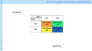
Confusion Matrix-based Metrics. These also take into account True Positive Rate (TPR), True
Negative Rate (TNR), False Positive Rate (FPR),and False Negative Rate (FNR)
Parity-based Metrics. They consider the predicted positive rates across different groups

16. 16
<event
name>
Error types in binary prediction
Sensitivity
Specificity

17. 17
<event
name>
Parity-based: Demographic Parity
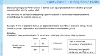
Statistical/Demographic Parity: fairness is defined as an equal probability between the two groups of
being classified with the positive label.
The probability for an instance of receiving a positive outcome is conditionally independent of the
protected group the instance belongs to:
Example: If 15% of applicants from g0 are approved for loans, then 15% of applicants from g1 should
also be approved, regardless of any differences in default rates between groups
Limitation:
Can lead to "reverse discrimination" if forced when underlying distributions differ significantly
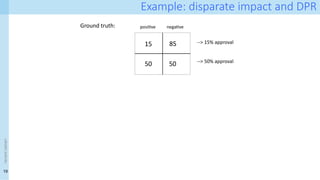
negative
positive
85
50
15 --> 15% approval
50 --> 50% approval
Default rates in
Training set:
Does not consider
correctness of predictions
Achieving demographic
parity may sacrifice accuracy

18. 18
<event
name> Parity-based: Disparate Impact / Demographic parity ratio
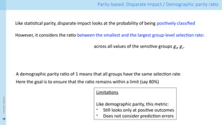
Like statistical parity, disparate impact looks at the probability of being positively classified
However, it considers the ratio between the smallest and the largest group-level selection rate:
A demographic parity ratio of 1 means that all groups have the same selection rate
Here the goal is to ensure that the ratio remains within a limit (say 80%)
Limitations
Like demographic parity, this metric:
- Still looks only at positive outcomes
- Does not consider prediction errors
across all values of the sensitive groups g0, g1.

19. 19
<event
name>
Example: disparate impact and DPR
negative
positive
85
50
15 --> 15% approval
50 --> 50% approval
Ground truth:

20. 20
<event
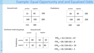
name> Confusion Matrix-based: Equal Opportunity and Equalized Odds
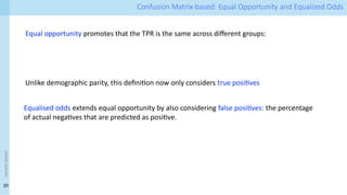
Equal opportunity promotes that the TPR is the same across different groups:
Unlike demographic parity, this definition now only considers true positives
Equalised odds extends equal opportunity by also considering false positives: the percentage
of actual negatives that are predicted as positive.

21. 21
<event
name>
Example: Equal Opportunity and and Equalized Odds
negative
positive
85
100
15
100
Ground truth:
185
115
100
200
negative
positive
40
100
60
100
Predictions:
160 140
100
200
negative
positive
10
Confusion matrix by group: Ground truth:
Predictions:
positive
negative
50
80
20
5 35 80
20
TPRG0 = 10 / (10+5) = .67
TPRG1 = 80 / (80+20) = .8
FPRG0 = 50 / (50+35) = .59
FPRG1 = 20 / (20+80) = .2

22. 22
<event
name>
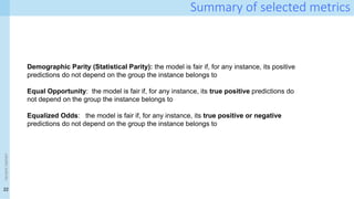
Summary of selected metrics
Demographic Parity (Statistical Parity): the model is fair if, for any instance, its positive
predictions do not depend on the group the instance belongs to
Equal Opportunity: the model is fair if, for any instance, its true positive predictions do
not depend on the group the instance belongs to
Equalized Odds: the model is fair if, for any instance, its true positive or negative
predictions do not depend on the group the instance belongs to

23. 23
<event
name>
Enforcing fairness
Source: [1]
We have seen that fairness does not occur “naturally” when training a classifier
- Imbalance between positive and negative outcomes within groups tends to translate into unfairness
How can we enforce fairness properties in our classifier, despite bias in the data?

24. 24
<event
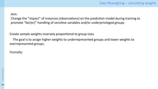
name> Data Reweighing – calculating weights
Create sample weights inversely proportional to group sizes
The goal is to assign higher weights to underrepresented groups and lower weights to
overrepresented groups.
Formally:
Aim:
Change the “impact” of instances (observations) on the prediction model during training to
promote “fair(er)” handling of sensitive variables and/or underprivileged groups

25. 25
<event
name>
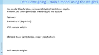
Data Reweighing – train a model using the weights
In a standard loss function, each example typically contributes equally.
However, this can be generalised to take weights into account
Standard MSE (Regression):
Standard Binary sigmoid cross-entropy (classification):
With example weights:
Examples:
With example weights:

26. 26
<event
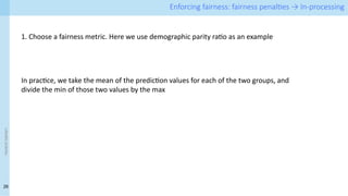
name> Enforcing fairness: fairness penalties → In-processing
1. Choose a fairness metric. Here we use demographic parity ratio as an example
In practice, we take the mean of the prediction values for each of the two groups, and
divide the min of those two values by the max

27. 27
<event
name> Enforcing fairness: fairness penalties → In-processing
2. Extend the standard loss function with a fairness regularization term
In this setting, regularization means adding penalty terms to penalize the classifier
Extending the classifier’s loss function with fairness terms seeks to balance fairness and accuracy
The fairness-accuracy trade-off parameter λ is crucial.
Larger values prioritize fairness over accuracy.
This is typically tuned through cross-validation and examining the Pareto front of the accuracy-
fairness trade-off

28. 28
<event
name>
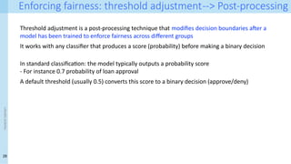
Enforcing fairness: threshold adjustment--> Post-processing
Threshold adjustment is a post-processing technique that modifies decision boundaries after a
model has been trained to enforce fairness across different groups
It works with any classifier that produces a score (probability) before making a binary decision
In standard classification: the model typically outputs a probability score
- For instance 0.7 probability of loan approval
A default threshold (usually 0.5) converts this score to a binary decision (approve/deny)

29. 29
<event
name> Enforcing fairness: threshold adjustment--> Post-processing
Instead of using a single threshold for all groups, we use group-specific thresholds
Each protected group gets its own optimized decision boundary
For two groups g0, g1 the goal is to find two thresholds t0, t1 such that the percentage of g0 with
scores ≥ t0 = percentage of g1 with scores ≥ t1
In practice-:
- Consider the group-specific scores s(g0), s(g1) for each of g0, g1. --> these are given by the
classifier
- Define the overall target rate q as the mean of the scores greater than the default
threshold 0.5 (positive scores)
- The threshold for group g is the q-th percentile of s(g)
[see notebook Adult-example, bottom for an example]

30. 30
<event
name>
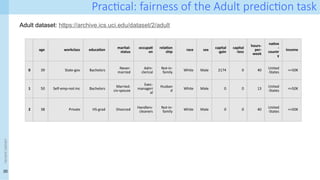
Practical: fairness of the Adult prediction task
Adult dataset: https://archive.ics.uci.edu/dataset/2/adult
age workclass education marital-
status
occupati
on
relation
ship
race sex capital
-gain
capital
-loss
hours-
per-
week
native
-
countr
y
income
0 39 State-gov Bachelors
Never-
married
Adm-
clerical
Not-in-
family
White Male 2174 0 40
United
-States
<=50K
1 50 Self-emp-not-inc Bachelors
Married-
civ-spouse
Exec-
manageri
al
Husban
d White Male 0 0 13
United
-States <=50K
2 38 Private HS-grad Divorced
Handlers-
cleaners
Not-in-
family White Male 0 0 40
United
-States <=50K

31. 31
<event
name>
Training a model… and making it fair
Data load Adult census dataset
- We use Sex as protected attribute
- Bit vector A identifies records in each group A = data['sex'].map({'Male': 1, 'Female':
0}).values
- Income (low/high) is the target variable
- Bit vector y identifies records in each class
y = data['income'].map({'>50K': 1, '<=50K': 0}).values
Normal data prep
- Separate covariates from target variable
- Scale numerical variables
Train logistic regression model
baseline_model = LogisticRegression(max_iter=1000)
baseline_model.fit(X_train, y_train)
y_pred_baseline = baseline_model.predict(X_test)
Notebook: Adult-example on Canvas

32. 32
<event
name>
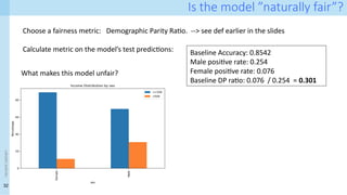
Is the model ”naturally fair”?
Choose a fairness metric: Demographic Parity Ratio. --> see def earlier in the slides
Calculate metric on the model’s test predictions: Baseline Accuracy: 0.8542
Male positive rate: 0.254
Female positive rate: 0.076
Baseline DP ratio: 0.076 / 0.254 = 0.301
What makes this model unfair?

33. 33
<event
name>
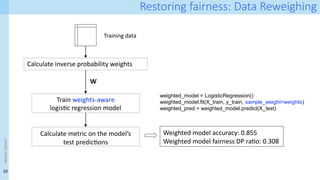
Restoring fairness: Data Reweighing
Calculate inverse probability weights
Training data
W
Train weights-aware
logistic regression model
weighted_model = LogisticRegression()
weighted_model.fit(X_train, y_train, sample_weight=weights)
weighted_pred = weighted_model.predict(X_test)
Weighted model accuracy: 0.855
Weighted model fairness DP ratio: 0.308
Calculate metric on the model’s
test predictions

34. 34
<event
name>
Restoring fairness: post-processing
male_scores = y_scores[A_test == 1]
female_scores = y_scores[A_test == 0]
Calculate per- group scores
Training data
W
Identify overall positive target rate
Find thresholds that match this
rate for each group
target_rate = np.mean(y_scores >= 0.5)
q = 100 * (1 - target_rate)
male_threshold = np.percentile(male_scores, q)
female_threshold = np.percentile(female_scores, q)
Apply separate thresholds to each
group
y_pred_fair[A_test == 1] = (male_scores >= male_threshold)
y_pred_fair[A_test == 0] = (female_scores >= female_threshold)
Fair Accuracy: 0.8285
Fair DP ratio: 0.9995
Male positive rate: 0.1942
Female positive rate: 0.1943

35. 35
<event
name>
Summary
Fairness can be defined rigorously and quantitatively for Classification problems and relative to
protected (or “sensitive”) attributes of the data
- We have explored the simplest: binary classification, one single binary protected attribute
In this framework we can define a number of fairness metrics
- Optimising the model for accuracy does not automatically enforce fairness
- Techniques have been developed to correct the model to ensure fairness. This may require
sacrificing accuracy
- We have presented examples of methods that operate
- pre-processing: modify the data
- In-processing: modify the loss function
- Post-processing: modify the decision thresholds