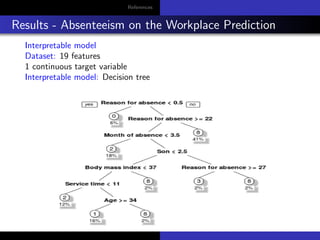
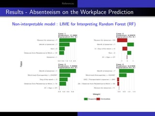
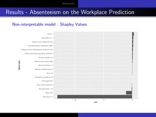
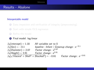
This presentation talks about some of the outstanding methods for Interpreting the complex machine learning black box models. One of the ideas is to use interpretable simple models to explain predictions using sophisticated black box machine learning models. Model Agnostic methods are proven to have some specific advantages over the Model Specific Methods of Interpretability. This work demonstrates some of such results.

1. Model Agnostic Methods for Interpretable Machine
Learning
Ankit Tewari, Carles Mitjans Coma & Tom´as Izquierdo
BarcelonaTech UPC FIB
Machine Learning project, March-June 2018

2. References
Introduction
ML is winning popularity: games, medical, driving, etc.
Black-Box models - Inner working
The necessity for interpretability comes from an incompleteness in
the problem formalisation [?], meaning that for certain problems or
tasks it is not enough to get the answer (the what). The model also
has to give an explanation how it came to the answer (the why),
because a correct prediction only partially solves your original
problem.
Aim of interpretation models - Control biased results
Minorities: winner takes it all.
Ethics: Job seeking, terrorist detection, etc.
Accuracy : when applying the model to real life - 99% accuracy
beacuse of test-validation. Existance of correlations that might not
ecists in real time.

3. References
Methods
Local Surrogate Models (LIME)
Feature Importance Plot
Shapley Values
Individual Conditional Expectation (ICE)

4. References
Methods
Local Surrogate Model (LIME)
We can describe the recipe for fitting local surrogate models as follows:
We first choose our instance (observations) of interest for which we
want to have an explanation of its black box prediction
Then we perturb our dataset and get the black box predictions for
these new points
We then weight the new samples by their proximity to the instance
of interest
Finally, we fit a weighted, interpretable model on the dataset with
the variations and explain prediction by interpreting the local model

5. References
Methods
Feature Importance
A feature’s importance is the increase in the modelˆas prediction
error after we permuted the feature’s values (breaks the
relationship between the feature and the outcome)
Input: Trained model ˆf , feature matrix X , target vector Y , error
measure L(Y , ˆY )
1. Estimate the original model error eorig (ˆf ) = L(Y , ˆf (X)) (e.g. mean
squared error)
2. For each feature j ∈ {1, ..., p} d
Generate feature matrix Xpermj
by permuting feature Xj in X. This
breaks the association between Xj and Y .
Estimate error eperm = L(Y , ˆf (Xpermj
)) based on the predictions of
the permuted data
Calculate permutation feature importance FIj = eperm(ˆf )/eorig (ˆf ) .
Alternatively, the difference can be used: FIj = eperm(ˆf ) − eorig (f )
3. Sort variables by descending FI.

6. References
Methods
Shapley Values
The Shapley value is the average marginal contribution of a
feature value over all possible coalitions.
Predictions can be explained by assuming that each feature is
a ’player’ in a game where the prediction is the payout. The
Shapley value - a method from coalitional game theory - tells
us how to fairly distribute the ’payout’ among the features.
The interpretation of the Shapley value. φij for feature j and
instance i is: the feature value xij contributed φij towards the
prediction for instance i compared to the average prediction
for the dataset. The Shapley value works for both classification (if
we deal with probabilities) and regression. We use the Shapley value
to analyse the predictions of a Random Forest model predicting the
absenteeism at workplace.

7. References
Methods
Individual Conditional Expectation (ICE)
The partial dependence plot (PDP) shows the marginal effect of a
feature on the predicted outcome of a previously fit model (J. H.
Friedman 2001). The prediction function is fixed at a few values of
the chosen features and averaged over the other features.
For a chosen feature, Individual Conditional Expectation (ICE) plots
draw one line per instance, representing how the instanceˆas
prediction changes when the feature changes. The partial
dependence plot for visualizing the average effect of a feature is a
global method, because it does not focus on specific instances, but
on an overall average. The equivalent to a PDP for local
expectations is called individual conditional expectation (ICE) plot

8. References
Results - Iris - Intepretable
Dataset: 4 features (sepal/petal length/width)
1 multilabel(setosa,versicolor,virginica)
Interpretable model: Decission Tree

9. References
Results - Iris - Non-Intepretable
Non-interpretable model: Random Forest

10. References
Results - Absenteeism on the Workplace Prediction
Interpretable model
Dataset: 19 features
1 continuous target variable
Interpretable model: Decision tree

11. References
Results - Absenteeism on the Workplace Prediction
Non-interpretable model : LIME for Gradient Boosting Machine (GBM)

12. References
Results - Absenteeism on the Workplace Prediction
Non-interpretable model : LIME for Interpreting Random Forest (RF)

13. References
Results - Absenteeism on the Workplace Prediction
Non-interpretable model: Feature Importance Plot using GBM

14. References
Results - Absenteeism on the Workplace Prediction
Non-interpretable model : Shapley Values

15. References
Results - Abalone
Interpretable model
1 Data inspection and verification of integrity (preprocessing)
2 Start with simple OLS regression
3 Refine the model
4 Final model: log-linear

16. References
Results - Abalone
Interpretable model
1 Data inspection and verification of integrity (preprocessing)
2 Start with simple OLS regression
3 Refine the model
4 Final model: log-linear

17. References
Results - Abalone
Interpretable model
1 Data inspection and verification of integrity (preprocessing)
2 Start with simple OLS regression
3 Refine the model
4 Final model: log-linear

18. References
Results - Abalone
Interpretable model
1 Data inspection and verification of integrity (preprocessing)
2 Start with simple OLS regression
3 Refine the model
4 Final model: log-linear
Rings = β0 + β1Sex(F) + β2Length + β3Diameter+
+ β4Height + β5Whole.weight + β6Shucked.weight+
+ β7Viscera.weight + β8Shell.weight
(1)

19. References
Results - Abalone
Interpretable model
1 Data inspection and verification of integrity (preprocessing)
2 Start with simple OLS regression
3 Refine the model
4 Final model: log-linear
log(Ringsi ) = 1.18 + (-0.1)Sex + 2.07Diameter +
+ 3.91Height + (-0.61) Viscera2 + Shell2 + Shucked2
(1)

20. References
Results - Abalone
Interpretable model
1 Data inspection and verification of integrity (preprocessing)
2 Start with simple OLS regression
3 Refine the model
4 Final model: log-linear
β0(intercept) = 1.18 All variables set to 0
β1(Sex) = −0.1 baseline : Infant | Grownup change : e−0.1
β2(Diameter) = 2.07 Factor change : e2.07
β3(Height) = 3.91 Factor change : e3.91
β4(
√
Viscera2 + Shell2 + Shucked2) = −0.61 Factor change : e−0.61

21. References
Results - Abalone
Non-interpretable model
1 Apply Random Forest
2 Visualize overall feature importance
3 Visualize single feature importance
4 Visualize overall feature interaction
5 Visualize single feature interaction

22. References
Results - Abalone
Non-interpretable model
1 Apply Random Forest
2 Visualize overall feature importance
3 Visualize single feature importance
4 Visualize overall feature interaction
5 Visualize single feature interaction

23. References
Conclusion & Future work
Conslusion
It would be interesting to observe that how the predictions can be
explained if tend to use a very complex neural network or any other
deep learning algorithm. In such a scenario, we can always rely on
LIME for giving us an insight about the local behaviour.
Future work
In the future, we aim to explore more on the idea of interpreting the
predictions for time series made by LSTM models as an example

24. References
References
References
1 European Union’s resource website to educate the public
about the main elements of the General Data Protection
Regulation (GDPR) - https://www.eugdpr.org/
2 Goodman, B. and Flaxman, S., 2016. European Union
regulations on algorithmic decision-making and a”right to
explanation”. arXiv preprint arXiv:1606.08813
3 Ribeiro, M.T., Singh, S. and Guestrin, C., 2016, August. Why
should i trust you?: Explaining the predictions of any classifier.
In Proceedings of the 22nd ACM SIGKDD International
Conference on Knowledge Discovery and Data Mining (pp.
1135-1144). ACM.
4 Interpretable Machine Learning: A Guide for Making Black
Box Models Explainable -
https://christophm.github.io/interpretable-ml-
book/agnostic.html