IJRET: International Journal of Research in Engineering and Technology eISSN: 2319-1163 | pISSN: 2321-7308
_______________________________________________________________________________________
Volume: 03 Issue: 05 | May-2014, Available @ http://www.ijret.org 665
A NEW NON-SYMMETRIC INFORMATION DIVERGENCE OF
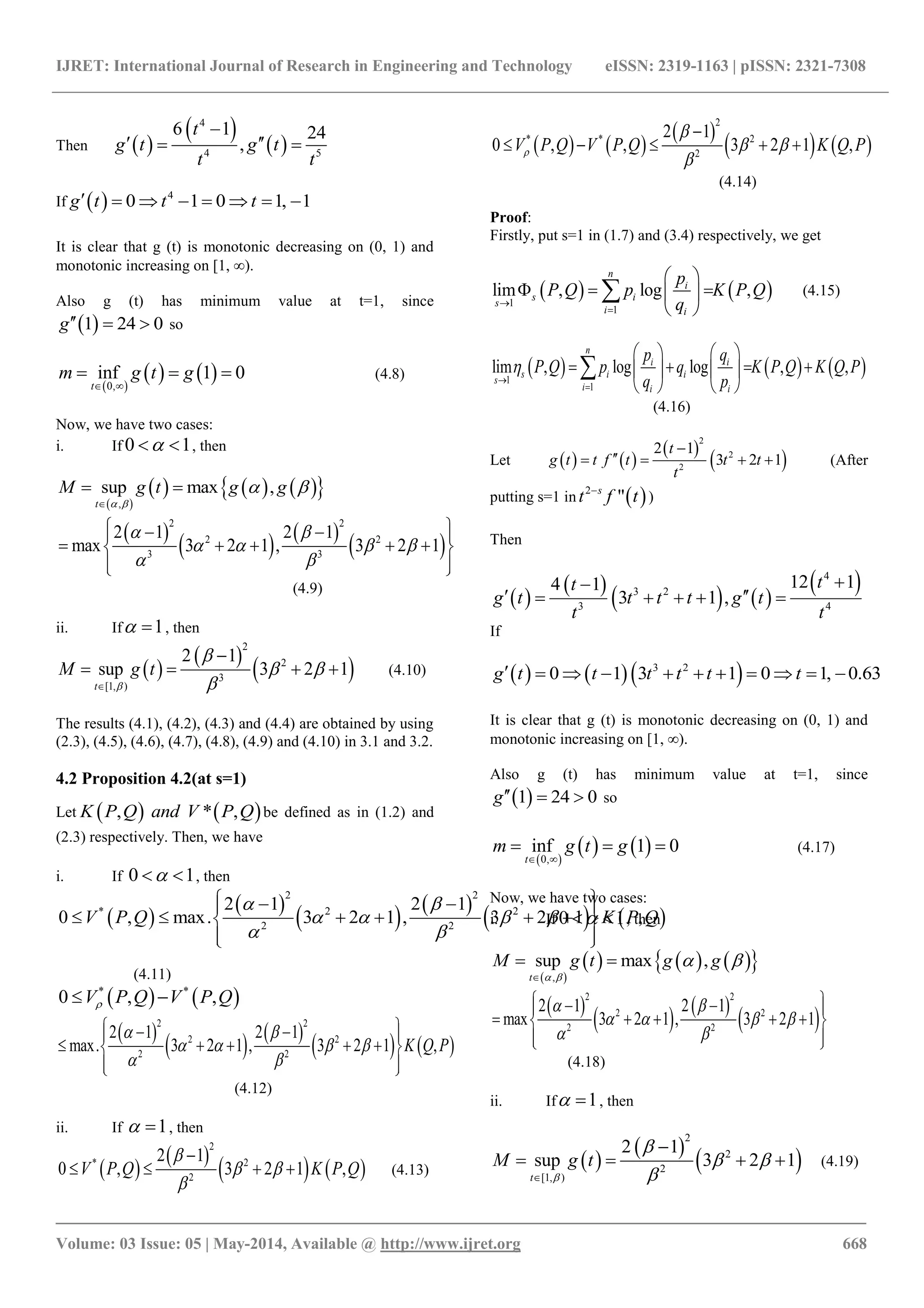
CSISZAR'S CLASS, PROPERTIES AND ITS BOUNDS
K.C.Jain1
, Praphull Chhabra2
1
Professor, Department of Mathematics, Malaviya National Institute of Technology, Jaipur (Rajasthan), India
2
Ph.d Scholar, Department of Mathematics, Malaviya National Institute of Technology, Jaipur (Rajasthan), India
Abstract
Non-parametric measures give the amount of information supplied by the data for discriminating in favor of a probability
distribution P against another Q , or for measuring the distance or affinity between P and Q .
There are several generalized functional divergences, such as: Csiszar divergence, Renyi- like divergence, Bregman divergence,
Burbea- Rao divergence etc. all. In this paper, a non-parametric non symmetric measure of divergence which belongs to the
family of Csiszár’s f-divergence is proposed. Its properties are studied and get the bounds in terms of some well known divergence
measures.
Mathematics Subject Classification: 94A17, 26D15
Keywords: Csiszar's f divergence, convex and normalized function, non-symmetric divergence measure, information
inequalities, bounds of divergence measure.
----------------------------------------------------------------------***-------------------------------------------------------------------
1. INTRODUCTION
Let  1 2 3
1
, , ..., : 0, 1 , 2
n
n n i i
i
P p p p p p p n

 
      
 

be the set of all complete finite discrete probability
distributions. If we take ip ≥0 for some 1, 2, 3,...,i n ,
then we have to suppose that  
0
0 0 0 0
0
f f
 
  
 
.
Csiszar [2], given the generalized f- divergence measure,
which is given by:
 
1
,
n
i
f i
i i
p
C P Q q f
q
 
  
 
 (1.1)
Where  : 0,f R  (set of real no.) is real, continuous
and convex function and
   1 2 3 1 2 3, , ..., , , , ...,n nP p p p p Q q q q q  ∈ Γn,
where ip and iq are probability mass functions. Many
known divergences can be obtained from this generalized
measure by suitably defining the convex function f. Some of
those are as follows:
  
1
, log
n
i
i
i i
p
K P Q p
q
 
  
 
 = Kullback- Leibler
divergence measure [4] (1.2)
  
 
2
2
1
,
n
i i
i i
p q
P Q
q



  = Chi- Square
divergence measure [5] (1.3)
  
 
2
1
,
2
n
i i
i
p q
h P Q


  = Hellinger
discrimination [3] (1.4)

   1
1
, , 1
an
i
a a
i i
p
R P Q a
q 

  = Renyi’s “a”
order entropy [6] (1.5)

  
1
,
n
i i
i
B P Q p q

  = Bhattacharya
divergence measure [1] (1.6)

Relative information of type “s” [9]
    
1 1
1
, 1 1 , 0,1
n
s s
s i i
i
P Q s s p q s and s R
 

 
         
 

(1.7)
IJRET: International Journal of Research in Engineering and Technology eISSN: 2319-1163 | pISSN: 2321-7308
_______________________________________________________________________________________
Volume: 03 Issue: 05 | May-2014, Available @ http://www.ijret.org 666
Particularly
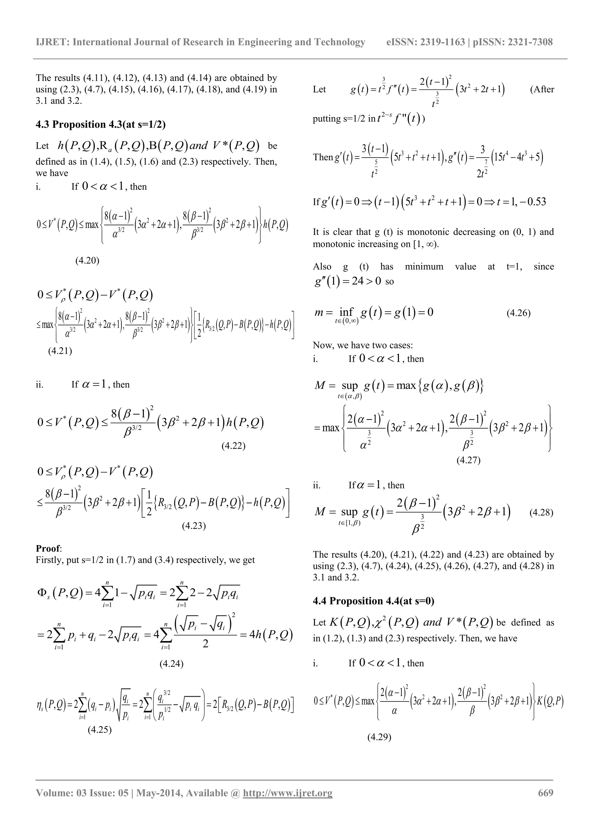
       1 0
lim , , , lim , ,s s
s s
P Q K P Q P Q K Q P
 
   
(1.8)
Where  ,K P Q is given by (1.2).
  
1
, log
2 2
n
i i i i
i i
p q p q
G P Q
p
   
   
   
 =
Relative AG Divergence [7] (1.9)
Similarly, we get many others divergences as well by
defining suitable convex function
2. NEW INFORMATION DIVERGENCE
MEASURE
In this section, we shall obtain a new divergence measure
corresponding to new convex function, and will study the
properties.
The following theorem is well known in literature [2].
Theorem 1: If the function f is convex and normalized, i.e.,
 1 0f  , then  ,fC P Q and its ad joint  ,fC Q P are
both non-negative and convex in the pair of probability
distribution  , n nP Q    .
Let f: (0, ∞) → R, be a mapping, defined as:
 
 
 
4
1
, 0,
t
f t t
t

   (2.1)
And
 
 
 
3
2
1
3 1
t
f t t
t

   ,  
 
 
2
2
3
2 1
3 2 1
t
f t t t
t

    (2.2)
Properties of function defined by (2.1), are as follows:
 Since      0 0,f t t f t      is a convex
function.
 Since    1 0f f t  is a normalized function.
 Since   0f t  at  0,1 and   0f t  at
   1, f t  is monotonically decreasing in
 0,1 and monotonically increasing in  1, , and
 1 0f   .
Fig1: Graph of convex function  f t
Now, put (2.1) in (1.1), we get the following new
divergence:
   
 
4
*
2
1
, ,
n
i i
f
i i i
p q
C P Q V P Q
p q

   (2.3)
Properties of divergence defined by (2.3), are as follows:
 In view of theorem 1, we can say that
 *
, 0V P Q  and convex in the pair of probability
distribution  , n nP Q    .
  *
, 0 i iV P Q if P Q or p q   (Attains its
minimum value).
 Since    * *
, ,V P Q V Q P   *
,V P Q is non-
symmetric divergence measure w.r.t. &P Q .
Figure 2 shows the behavior of  * ,V P Q , Relative
Arithmetic-Geometric divergence  ,G P Q and Kullback-
Leibler divergence  ,K P Q . We have considered
,1 1 ,( ) ( ) (0,1)i ip a a and q a a awhere     . It
2 4 6 8 10
100
200
300
400
500
600
700
0
1
2
3
4
5
6
0 0.5 1
a →
Figure 2: Comparison of divergence
measures
V*(P,Q)
Relative
Arithmetic
Geometric div.
Kullback-
Leibler div.
IJRET: International Journal of Research in Engineering and Technology eISSN: 2319-1163 | pISSN: 2321-7308
_______________________________________________________________________________________
Volume: 03 Issue: 05 | May-2014, Available @ http://www.ijret.org 667
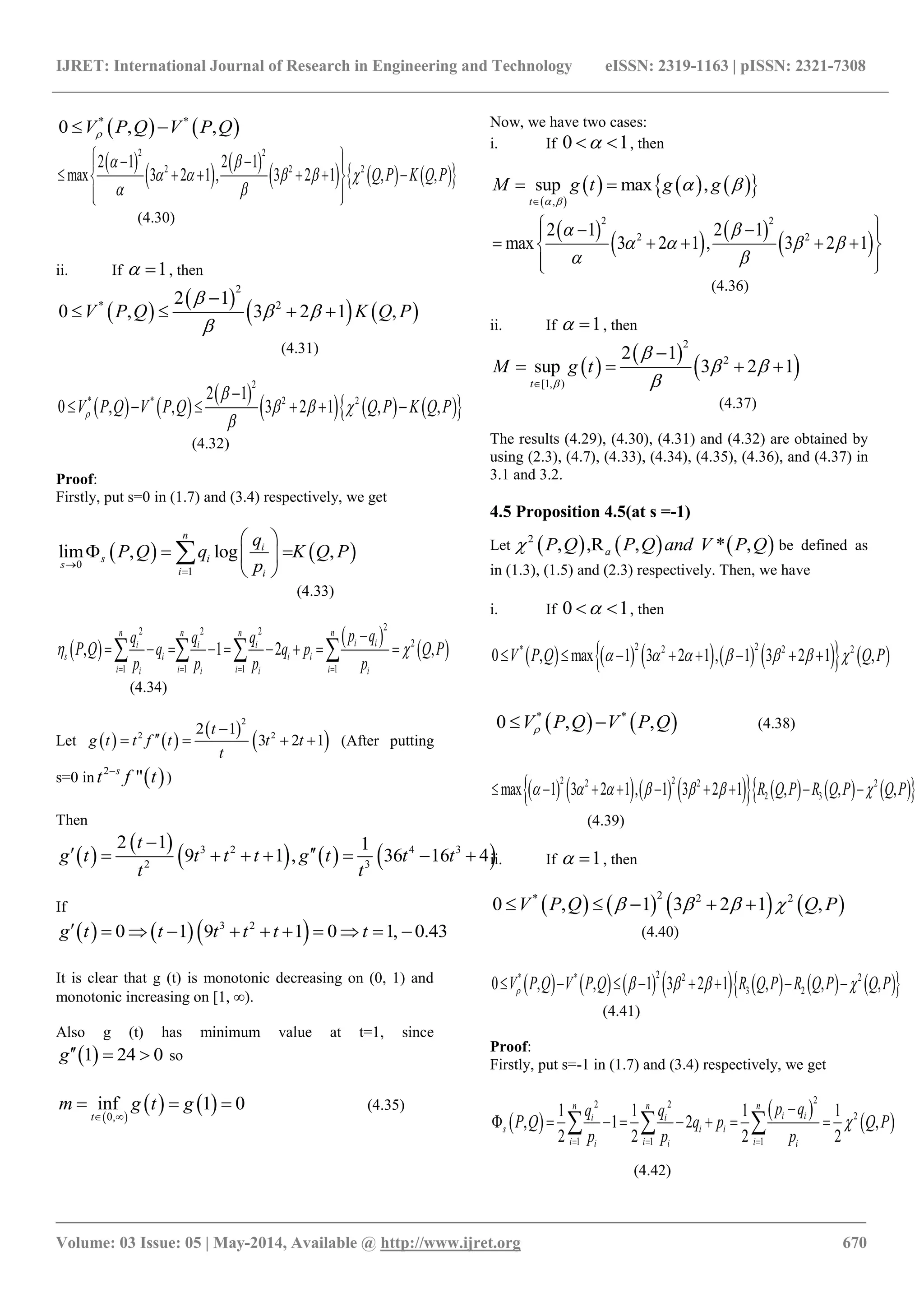
is clear from figure 2 that the new measure  *
,V P Q has a
steeper slope then    , ,G P Q and K P Q .
3. CSISZAR’S FUNCTIONAL DIVERGENCE
AND INEQUALITIES
The following theorem is well known in literature [8].
Theorem 2: Let :f I R R  (I is an open interval) be
a mapping which is normalized, i.e.,  1 0f  and suppose
that
I. f is twice differentiable on
 , , 0 1 with           .
II. There exist real constants ,m M such that
   2
" ,s
tm M and m t f M t and s R 
     
and
If , 0 1,2,3...,i
n
i
p
P Q with i n
q
        
, then
     , , ,s f sm P Q C P Q M P Q    (3.1)
And
           , , , , , ,s ss f sm P Q P Q C P Q C P Q M P Q P Q           
(3.2)
Where
     
2
1
, , ,
n
i
f f i i
i i
pP
C P Q C P C P Q p q f
Q q
  

  
      
   

(3.3)
       
1
2
1
1
, , , 1 , 1s s
s
n
i
s i i
i i
pP
P Q C P C P Q s p q s
Q q



  

  
       
   

(3.4)
And    , , ,f sC P Q P Q are given by (1.1) and (1.7)
respectively
4. BOUNDS OF NEW INFORMATION
DIVERGENCE MEASURE
In this section, we derive bounds for  *
,V P Q in terms of
the well known divergences in the following propositions at
2,1,1/ 2, 0 1s and  , by using the theorem 2.
4.1 Proposition 4.1(at s=2)
Let    2
, * ,P Q and V P Q be defined as in (1.3) and
(2.3) respectively. Then, we have
i. If 0 1  , then
 
 
   
   
2 2
* 2 2 2
3 3
1 1
0 , max. 3 2 1 , 3 2 1 ,V P Q P Q
 
    
 
   
      
  
   * *
0 , ,V P Q V P Q  (4.1)
 
   
   
2 2
2 2 2
3 3
1 1
max. 3 2 1 , 3 2 1 ,P Q
 
    
 
   
     
  
(4.2)
ii. If 1  , then
 
 
   
2
* 2 2
3
1
0 , 3 2 1 ,V P Q P Q

  


    (4.3)
   
 
   
2
* * 2 2
3
1
0 , , 3 2 1 ,V P Q V P Q P Q

  


    
(4.4)
Proof:
Firstly, put s=2 in (1.7) and (3.4) respectively, we get
 
 
 
22 2
2
1 1 1
1 1 1 1
, 1 2 ,
2 2 2 2
n n n
i ii i
s i i
i i ii i i
p qp p
P Q p q P Q
q q q

  

         
(4.5)
   
2 2
1 1 1
, 1
n n n
i i i
s i i i
i i ii i i
p p p
P Q p q p
q q q

  
       
 
 
22
2
1 1
2 ,
n n
i ii
i i
i ii i
p qp
p q P Q
q q

 

     
(4.6)
And by putting  f t in (3.3), we get
   
 
 
 
42
* * *
2
1
, , , 3
n
i i
f f i i
i i i
p qP
V P Q V P V P Q p q
Q p q
  

 
    
 

(4.7)
Let    
 
 
2
2
3
2 1
3 2 1
t
g t f t t t
t

    (After
putting s=2 in  2
"s
t tf
)
IJRET: International Journal of Research in Engineering and Technology eISSN: 2319-1163 | pISSN: 2321-7308
_______________________________________________________________________________________
Volume: 03 Issue: 05 | May-2014, Available @ http://www.ijret.org 668
Then  
 
 
4
4 5
6 1 24
,
t
g t g t
t t

  
If   4
0 1 0 1, 1g t t t       
It is clear that g (t) is monotonic decreasing on (0, 1) and
monotonic increasing on [1, ∞).
Also g (t) has minimum value at t=1, since
 1 24 0g   so
 
   0,
inf 1 0
t
m g t g
 
   (4.8)
Now, we have two cases:
i. If 0 1  , then
 
      ,
sup max ,
t
M g t g g
 
 

 
 
   
 
2 2
2 2
3 3
2 1 2 1
max 3 2 1 , 3 2 1
 
   
 
   
     
  
(4.9)
ii. If 1  , then
 
 
 
2
2
3
[1, )
2 1
sup 3 2 1
t
M g t


 


    (4.10)
The results (4.1), (4.2), (4.3) and (4.4) are obtained by using
(2.3), (4.5), (4.6), (4.7), (4.8), (4.9) and (4.10) in 3.1 and 3.2.
4.2 Proposition 4.2(at s=1)
Let    , * ,P Q and V PK Q be defined as in (1.2) and
(2.3) respectively. Then, we have
i. If 0 1  , then
 
 
   
   
2 2
* 2 2
2 2
2 1 2 1
0 , max. 3 2 1 , 3 2 1 ,V P Q K P Q
 
   
 
   
      
  
(4.11)
   * *
0 , ,V P Q V P Q 
 
   
   
2 2
2 2
2 2
2 1 2 1
max. 3 2 1 , 3 2 1 ,K Q P
 
   
 
   
     
  
(4.12)
ii. If 1  , then
 
 
   
2
* 2
2
2 1
0 , 3 2 1 ,V P Q K P Q

 


    (4.13)
   
 
   
2
* * 2
2
2 1
0 , , 3 2 1 ,V P Q V P Q K Q P

 


    
(4.14)
Proof:
Firstly, put s=1 in (1.7) and (3.4) respectively, we get
   1
1
lim , log ,
n
i
s i
s
i i
p
P Q p K P Q
q

 
   
 
 (4.15)
     1
1
lim , log log , ,
n
i i
s i i
s
i i i
p q
P Q p q K P Q K Q P
q p



   
      
   

(4.16)
Let    
 
 
2
2
2
2 1
3 2 1
t
g t t f t t t
t

    (After
putting s=1 in  2
"s
t tf
)
Then
 
 
   
 4
3 2
3 4
12 14 1
3 1 ,
tt
g t t t t g t
t t

     
If
    3 2
0 1 3 1 0 1, 0.63g t t t t t t          
It is clear that g (t) is monotonic decreasing on (0, 1) and
monotonic increasing on [1, ∞).
Also g (t) has minimum value at t=1, since
 1 24 0g   so
 
   0,
inf 1 0
t
m g t g
 
   (4.17)
Now, we have two cases:
i. If 0 1  , then
 
      ,
sup max ,
t
M g t g g
 
 

 
 
   
 
2 2
2 2
2 2
2 1 2 1
max 3 2 1 , 3 2 1
 
   
 
   
     
  
(4.18)
ii. If 1  , then
 
 
 
2
2
2
[1, )
2 1
sup 3 2 1
t
M g t


 


    (4.19)
IJRET: International Journal of Research in Engineering and Technology eISSN: 2319-1163 | pISSN: 2321-7308
_______________________________________________________________________________________
Volume: 03 Issue: 05 | May-2014, Available @ http://www.ijret.org 669
The results (4.11), (4.12), (4.13) and (4.14) are obtained by
using (2.3), (4.7), (4.15), (4.16), (4.17), (4.18), and (4.19) in
3.1 and 3.2.
4.3 Proposition 4.3(at s=1/2)
Let        ,R, * ,,B, ,ah P Q PP Q and V PQ Q be
defined as in (1.4), (1.5), (1.6) and (2.3) respectively. Then,
we have
i. If 0 1  , then
 
 
   
   
2 2
* 2 2
3/2 3/2
8 1 8 1
0 , max 3 2 1 , 3 2 1 ,V P Q h P Q
 
   
 
   
      
  
(4.20)
   * *
0 , ,V P Q V P Q 
 
   
        
2 2
2 2
3/23/2 3/2
8 1 8 1 1
max 3 2 1 , 3 2 1 , , ,
2
R Q P B P Q h P Q
 
   
 
    
           
(4.21)
ii. If 1  , then
 
 
   
2
* 2
3/2
8 1
0 , 3 2 1 ,V P Q h P Q

 


   
(4.22)
   * *
0 , ,V P Q V P Q 
 
        
2
2
3/23/2
8 1 1
3 2 1 , , ,
2
R Q P B P Q h P Q

 

  
      
(4.23)
Proof:
Firstly, put s=1/2 in (1.7) and (3.4) respectively, we get
 
1 1
, 4 1 2 2 2
n n
s i i i i
i i
P Q p q p q
 
     
   
2
1 1
2 2 4 4 ,
2
n n
i i
i i i i
i i
p q
p q p q h P Q
 

     
(4.24)
       
3/2
3/21/2
1 1
, 2 2 2 , ,
n n
i i
s i i i i
i ii i
q q
P Q q p p q R Q P B P Q
p p

 
 
         
 
 
(4.25)
Let    
 
 
23
22
3
2
2 1
3 2 1
t
g t t f t t t
t

    (After
putting s=1/2 in  2
"s
t tf
)
Then  
 
     3 2 4 3
5 7
2 2
3 1 3
5 1 , 15 4 5
2
t
g t t t t g t t t
t t

       
If     3 2
0 1 5 1 0 1, 0.53g t t t t t t          
It is clear that g (t) is monotonic decreasing on (0, 1) and
monotonic increasing on [1, ∞).
Also g (t) has minimum value at t=1, since
 1 24 0g   so
 
   0,
inf 1 0
t
m g t g
 
   (4.26)
Now, we have two cases:
i. If 0 1  , then
 
      ,
sup max ,
t
M g t g g
 
 

 
 
   
 
2 2
2 2
3 3
2 2
2 1 2 1
max 3 2 1 , 3 2 1
 
   
 
 
  
     
 
 
(4.27)
ii. If 1  , then
 
 
 
2
2
3
[1, )
2
2 1
sup 3 2 1
t
M g t


 



    (4.28)
The results (4.20), (4.21), (4.22) and (4.23) are obtained by
using (2.3), (4.7), (4.24), (4.25), (4.26), (4.27), and (4.28) in
3.1 and 3.2.
4.4 Proposition 4.4(at s=0)
Let      2
, , ,, *P Q and VK P Q P Q be defined as
in (1.2), (1.3) and (2.3) respectively. Then, we have
i. If 0 1  , then
 
 
   
   
2 2
* 2 22 1 2 1
0 , max 3 2 1 , 3 2 1 ,V P Q K Q P
 
   
 
   
      
  
(4.29)
IJRET: International Journal of Research in Engineering and Technology eISSN: 2319-1163 | pISSN: 2321-7308
_______________________________________________________________________________________
Volume: 03 Issue: 05 | May-2014, Available @ http://www.ijret.org 670
   * *
0 , ,V P Q V P Q 
 
   
      
2 2
2 2 22 1 2 1
max 3 2 1 , 3 2 1 , ,Q P K Q P
 
    
 
   
      
  
(4.30)
ii. If 1  , then
 
 
   
2
* 22 1
0 , 3 2 1 ,V P Q K Q P

 


   
(4.31)
   
 
      
2
* * 2 22 1
0 , , 3 2 1 , ,V P Q V P Q Q P K Q P

  


     
(4.32)
Proof:
Firstly, put s=0 in (1.7) and (3.4) respectively, we get
   0
1
lim , log ,
n
i
s i
s
i i
q
P Q q K Q P
p

 
   
 

(4.33)
 
 
 
22 2 2
2
1 1 1 1
, 1 2 ,
n n n n
i ii i i
s i i i
i i i ii i i i
p qq q q
P Q q q p Q P
p p p p
 
   

           
(4.34)
Let    
 
 
2
2 22 1
3 2 1
t
g t t f t t t
t

    (After putting
s=0 in  2
"s
t tf
)
Then
 
 
     3 2 4 3
2 3
2 1 1
9 1 , 36 16 4
t
g t t t t g t t t
t t

       
If
    3 2
0 1 9 1 0 1, 0.43g t t t t t t          
It is clear that g (t) is monotonic decreasing on (0, 1) and
monotonic increasing on [1, ∞).
Also g (t) has minimum value at t=1, since
 1 24 0g   so
 
   0,
inf 1 0
t
m g t g
 
   (4.35)
Now, we have two cases:
i. If 0 1  , then
 
      ,
sup max ,
t
M g t g g
 
 

 
 
   
 
2 2
2 22 1 2 1
max 3 2 1 , 3 2 1
 
   
 
   
     
  
(4.36)
ii. If 1  , then
 
 
 
2
2
[1, )
2 1
sup 3 2 1
t
M g t


 


   
(4.37)
The results (4.29), (4.30), (4.31) and (4.32) are obtained by
using (2.3), (4.7), (4.33), (4.34), (4.35), (4.36), and (4.37) in
3.1 and 3.2.
4.5 Proposition 4.5(at s =-1)
Let      2
,, * ,R ,a P QP Q and V P Q be defined as
in (1.3), (1.5) and (2.3) respectively. Then, we have
i. If 0 1  , then
            
2 2* 2 2 2
0 , max 1 3 2 1 , 1 3 2 1 ,V P Q Q P             
   * *
0 , ,V P Q V P Q  (4.38)
               2 22 2 2
2 3max 1 3 2 1 , 1 3 2 1 , , ,R Q P R Q P Q P              
(4.39)
ii. If 1  , then
       
2* 2 2
0 , 1 3 2 1 ,V P Q Q P       
(4.40)
              2* * 2 2
3 20 , , 1 3 2 1 , , ,V P Q V P Q R Q P R Q P Q P           
(4.41)
Proof:
Firstly, put s=-1 in (1.7) and (3.4) respectively, we get
 
 
 
22 2
2
1 1 1
1 1 1 1
, 1 2 ,
2 2 2 2
n n n
i ii i
s i i
i i ii i i
p qq q
P Q q p Q P
p p p

  

         
(4.42)
IJRET: International Journal of Research in Engineering and Technology eISSN: 2319-1163 | pISSN: 2321-7308
_______________________________________________________________________________________
Volume: 03 Issue: 05 | May-2014, Available @ http://www.ijret.org 671
       
2 3 2
3 22 2
1 1
1 1 1
, , ,
2 2 2
n n
i i i
s i i
i ii i i
q q q
P Q q p R Q P R Q P
p p p

 
 
         
 
 
(4.43)
Let        23 2
2 1 3 2 1g t t f t t t t     (After putting
s=-1 in  2
"s
t tf
)
Then      2 2
24 1 , 72 48g t t t g t t t    
If   0 0,1g t t   
It is clear that g (t) is monotonic decreasing on (0, 1) and
monotonic increasing on [1, ∞).
Also g (t) has minimum value at t=1, since
 1 24 0g   so
 
   0,
inf 1 0
t
m g t g
 
   (4.44)
Now, we have two cases:
i. If 0 1  , then
 
      ,
sup max ,
t
M g t g g
 
 

 
        2 22 2
max 2 1 3 2 1 ,2 1 3 2 1           
(4.45)
ii. If 1  , then
     2 2
[1, )
sup 2 1 3 2 1
t
M g t

  

    
(4.46)
The results (4.38), (4.39), (4.40) and (4.41) are obtained by
using (2.3), (4.7), (4.42), (4.43), (4.44), (4.45), and (4.46) in
3.1 and 3.2.
REFERENCES
[1]. Bhattacharyya A., “On some analogues to the amount of
information and their uses in statistical estimation”,
Sankhya, 8, 1-14.
[2]. Csiszar I., “Information type measures of differences of
probability distribution and indirect observations”, Studia
Math. Hungarica, 2(1967), 299-318.
[3]. Hellinger E., “Neue begrundung der theorie der
quadratischen formen von unendlichen vielen
veranderlichen”, J. Rein.Aug. Math., 136(1909), 210-271.
[4]. Kullback S. and Leibler R.A., “On Information and
Sufficiency”, Ann. Math. Statist., 22(1951), 79-86.
[5]. Pearson K., “On the Criterion that a given system of
deviations from the probable in the case of correlated system
of variables is such that it can be reasonable supposed to
have arisen from random sampling”, Phil. Mag., 50(1900),
157-172.
[6]. Renyi A., “On measures of entropy and information”,
Proc. 4th Berkeley Symposium on Math. Statist. and Prob.,
1(1961), 547-561.
[7]. Taneja I.J., New developments in generalized
information measures, Chapter in: Advances in Imaging and
Electron Physics, Ed. P.W. Hawkes, 91(1995), 37-135.
[8]. Taneja I. J. and Kumar P., “Generalized non-symmetric
divergence measures and inequalities” (2000), The Natural
Science and Engineering Research Council’s Discovery
grant to Pranesh Kumar.
[9]. Taneja I.J. and Kumar P., "Relative Information of type-
s, Csiszar's f-divergence and information inequalities",
Information Sciences, (2003).

A new non symmetric information divergence of

  • 1.
    IJRET: International Journalof Research in Engineering and Technology eISSN: 2319-1163 | pISSN: 2321-7308 _______________________________________________________________________________________ Volume: 03 Issue: 05 | May-2014, Available @ http://www.ijret.org 665 A NEW NON-SYMMETRIC INFORMATION DIVERGENCE OF CSISZAR'S CLASS, PROPERTIES AND ITS BOUNDS K.C.Jain1 , Praphull Chhabra2 1 Professor, Department of Mathematics, Malaviya National Institute of Technology, Jaipur (Rajasthan), India 2 Ph.d Scholar, Department of Mathematics, Malaviya National Institute of Technology, Jaipur (Rajasthan), India Abstract Non-parametric measures give the amount of information supplied by the data for discriminating in favor of a probability distribution P against another Q , or for measuring the distance or affinity between P and Q . There are several generalized functional divergences, such as: Csiszar divergence, Renyi- like divergence, Bregman divergence, Burbea- Rao divergence etc. all. In this paper, a non-parametric non symmetric measure of divergence which belongs to the family of Csiszár’s f-divergence is proposed. Its properties are studied and get the bounds in terms of some well known divergence measures. Mathematics Subject Classification: 94A17, 26D15 Keywords: Csiszar's f divergence, convex and normalized function, non-symmetric divergence measure, information inequalities, bounds of divergence measure. ----------------------------------------------------------------------***------------------------------------------------------------------- 1. INTRODUCTION Let  1 2 3 1 , , ..., : 0, 1 , 2 n n n i i i P p p p p p p n              be the set of all complete finite discrete probability distributions. If we take ip ≥0 for some 1, 2, 3,...,i n , then we have to suppose that   0 0 0 0 0 0 f f        . Csiszar [2], given the generalized f- divergence measure, which is given by:   1 , n i f i i i p C P Q q f q         (1.1) Where  : 0,f R  (set of real no.) is real, continuous and convex function and    1 2 3 1 2 3, , ..., , , , ...,n nP p p p p Q q q q q  ∈ Γn, where ip and iq are probability mass functions. Many known divergences can be obtained from this generalized measure by suitably defining the convex function f. Some of those are as follows:    1 , log n i i i i p K P Q p q         = Kullback- Leibler divergence measure [4] (1.2)      2 2 1 , n i i i i p q P Q q      = Chi- Square divergence measure [5] (1.3)      2 1 , 2 n i i i p q h P Q     = Hellinger discrimination [3] (1.4)     1 1 , , 1 an i a a i i p R P Q a q     = Renyi’s “a” order entropy [6] (1.5)     1 , n i i i B P Q p q    = Bhattacharya divergence measure [1] (1.6)  Relative information of type “s” [9]      1 1 1 , 1 1 , 0,1 n s s s i i i P Q s s p q s and s R                   (1.7)
  • 2.
    IJRET: International Journalof Research in Engineering and Technology eISSN: 2319-1163 | pISSN: 2321-7308 _______________________________________________________________________________________ Volume: 03 Issue: 05 | May-2014, Available @ http://www.ijret.org 666 Particularly        1 0 lim , , , lim , ,s s s s P Q K P Q P Q K Q P       (1.8) Where  ,K P Q is given by (1.2).    1 , log 2 2 n i i i i i i p q p q G P Q p              = Relative AG Divergence [7] (1.9) Similarly, we get many others divergences as well by defining suitable convex function 2. NEW INFORMATION DIVERGENCE MEASURE In this section, we shall obtain a new divergence measure corresponding to new convex function, and will study the properties. The following theorem is well known in literature [2]. Theorem 1: If the function f is convex and normalized, i.e.,  1 0f  , then  ,fC P Q and its ad joint  ,fC Q P are both non-negative and convex in the pair of probability distribution  , n nP Q    . Let f: (0, ∞) → R, be a mapping, defined as:       4 1 , 0, t f t t t     (2.1) And       3 2 1 3 1 t f t t t     ,       2 2 3 2 1 3 2 1 t f t t t t      (2.2) Properties of function defined by (2.1), are as follows:  Since      0 0,f t t f t      is a convex function.  Since    1 0f f t  is a normalized function.  Since   0f t  at  0,1 and   0f t  at    1, f t  is monotonically decreasing in  0,1 and monotonically increasing in  1, , and  1 0f   . Fig1: Graph of convex function  f t Now, put (2.1) in (1.1), we get the following new divergence:       4 * 2 1 , , n i i f i i i p q C P Q V P Q p q     (2.3) Properties of divergence defined by (2.3), are as follows:  In view of theorem 1, we can say that  * , 0V P Q  and convex in the pair of probability distribution  , n nP Q    .   * , 0 i iV P Q if P Q or p q   (Attains its minimum value).  Since    * * , ,V P Q V Q P   * ,V P Q is non- symmetric divergence measure w.r.t. &P Q . Figure 2 shows the behavior of  * ,V P Q , Relative Arithmetic-Geometric divergence  ,G P Q and Kullback- Leibler divergence  ,K P Q . We have considered ,1 1 ,( ) ( ) (0,1)i ip a a and q a a awhere     . It 2 4 6 8 10 100 200 300 400 500 600 700 0 1 2 3 4 5 6 0 0.5 1 a → Figure 2: Comparison of divergence measures V*(P,Q) Relative Arithmetic Geometric div. Kullback- Leibler div.
  • 3.
    IJRET: International Journalof Research in Engineering and Technology eISSN: 2319-1163 | pISSN: 2321-7308 _______________________________________________________________________________________ Volume: 03 Issue: 05 | May-2014, Available @ http://www.ijret.org 667 is clear from figure 2 that the new measure  * ,V P Q has a steeper slope then    , ,G P Q and K P Q . 3. CSISZAR’S FUNCTIONAL DIVERGENCE AND INEQUALITIES The following theorem is well known in literature [8]. Theorem 2: Let :f I R R  (I is an open interval) be a mapping which is normalized, i.e.,  1 0f  and suppose that I. f is twice differentiable on  , , 0 1 with           . II. There exist real constants ,m M such that    2 " ,s tm M and m t f M t and s R        and If , 0 1,2,3...,i n i p P Q with i n q          , then      , , ,s f sm P Q C P Q M P Q    (3.1) And            , , , , , ,s ss f sm P Q P Q C P Q C P Q M P Q P Q            (3.2) Where       2 1 , , , n i f f i i i i pP C P Q C P C P Q p q f Q q                    (3.3)         1 2 1 1 , , , 1 , 1s s s n i s i i i i pP P Q C P C P Q s p q s Q q                        (3.4) And    , , ,f sC P Q P Q are given by (1.1) and (1.7) respectively 4. BOUNDS OF NEW INFORMATION DIVERGENCE MEASURE In this section, we derive bounds for  * ,V P Q in terms of the well known divergences in the following propositions at 2,1,1/ 2, 0 1s and  , by using the theorem 2. 4.1 Proposition 4.1(at s=2) Let    2 , * ,P Q and V P Q be defined as in (1.3) and (2.3) respectively. Then, we have i. If 0 1  , then             2 2 * 2 2 2 3 3 1 1 0 , max. 3 2 1 , 3 2 1 ,V P Q P Q                           * * 0 , ,V P Q V P Q  (4.1)           2 2 2 2 2 3 3 1 1 max. 3 2 1 , 3 2 1 ,P Q                       (4.2) ii. If 1  , then         2 * 2 2 3 1 0 , 3 2 1 ,V P Q P Q           (4.3)           2 * * 2 2 3 1 0 , , 3 2 1 ,V P Q V P Q P Q            (4.4) Proof: Firstly, put s=2 in (1.7) and (3.4) respectively, we get       22 2 2 1 1 1 1 1 1 1 , 1 2 , 2 2 2 2 n n n i ii i s i i i i ii i i p qp p P Q p q P Q q q q                (4.5)     2 2 1 1 1 , 1 n n n i i i s i i i i i ii i i p p p P Q p q p q q q                 22 2 1 1 2 , n n i ii i i i ii i p qp p q P Q q q           (4.6) And by putting  f t in (3.3), we get           42 * * * 2 1 , , , 3 n i i f f i i i i i p qP V P Q V P V P Q p q Q p q               (4.7) Let         2 2 3 2 1 3 2 1 t g t f t t t t      (After putting s=2 in  2 "s t tf )
  • 4.
    IJRET: International Journalof Research in Engineering and Technology eISSN: 2319-1163 | pISSN: 2321-7308 _______________________________________________________________________________________ Volume: 03 Issue: 05 | May-2014, Available @ http://www.ijret.org 668 Then       4 4 5 6 1 24 , t g t g t t t     If   4 0 1 0 1, 1g t t t        It is clear that g (t) is monotonic decreasing on (0, 1) and monotonic increasing on [1, ∞). Also g (t) has minimum value at t=1, since  1 24 0g   so      0, inf 1 0 t m g t g      (4.8) Now, we have two cases: i. If 0 1  , then         , sup max , t M g t g g                2 2 2 2 3 3 2 1 2 1 max 3 2 1 , 3 2 1                      (4.9) ii. If 1  , then       2 2 3 [1, ) 2 1 sup 3 2 1 t M g t           (4.10) The results (4.1), (4.2), (4.3) and (4.4) are obtained by using (2.3), (4.5), (4.6), (4.7), (4.8), (4.9) and (4.10) in 3.1 and 3.2. 4.2 Proposition 4.2(at s=1) Let    , * ,P Q and V PK Q be defined as in (1.2) and (2.3) respectively. Then, we have i. If 0 1  , then             2 2 * 2 2 2 2 2 1 2 1 0 , max. 3 2 1 , 3 2 1 ,V P Q K P Q                       (4.11)    * * 0 , ,V P Q V P Q            2 2 2 2 2 2 2 1 2 1 max. 3 2 1 , 3 2 1 ,K Q P                      (4.12) ii. If 1  , then         2 * 2 2 2 1 0 , 3 2 1 ,V P Q K P Q          (4.13)           2 * * 2 2 2 1 0 , , 3 2 1 ,V P Q V P Q K Q P           (4.14) Proof: Firstly, put s=1 in (1.7) and (3.4) respectively, we get    1 1 lim , log , n i s i s i i p P Q p K P Q q           (4.15)      1 1 lim , log log , , n i i s i i s i i i p q P Q p q K P Q K Q P q p                    (4.16) Let         2 2 2 2 1 3 2 1 t g t t f t t t t      (After putting s=1 in  2 "s t tf ) Then          4 3 2 3 4 12 14 1 3 1 , tt g t t t t g t t t        If     3 2 0 1 3 1 0 1, 0.63g t t t t t t           It is clear that g (t) is monotonic decreasing on (0, 1) and monotonic increasing on [1, ∞). Also g (t) has minimum value at t=1, since  1 24 0g   so      0, inf 1 0 t m g t g      (4.17) Now, we have two cases: i. If 0 1  , then         , sup max , t M g t g g                2 2 2 2 2 2 2 1 2 1 max 3 2 1 , 3 2 1                      (4.18) ii. If 1  , then       2 2 2 [1, ) 2 1 sup 3 2 1 t M g t           (4.19)
  • 5.
    IJRET: International Journalof Research in Engineering and Technology eISSN: 2319-1163 | pISSN: 2321-7308 _______________________________________________________________________________________ Volume: 03 Issue: 05 | May-2014, Available @ http://www.ijret.org 669 The results (4.11), (4.12), (4.13) and (4.14) are obtained by using (2.3), (4.7), (4.15), (4.16), (4.17), (4.18), and (4.19) in 3.1 and 3.2. 4.3 Proposition 4.3(at s=1/2) Let        ,R, * ,,B, ,ah P Q PP Q and V PQ Q be defined as in (1.4), (1.5), (1.6) and (2.3) respectively. Then, we have i. If 0 1  , then             2 2 * 2 2 3/2 3/2 8 1 8 1 0 , max 3 2 1 , 3 2 1 ,V P Q h P Q                       (4.20)    * * 0 , ,V P Q V P Q                 2 2 2 2 3/23/2 3/2 8 1 8 1 1 max 3 2 1 , 3 2 1 , , , 2 R Q P B P Q h P Q                          (4.21) ii. If 1  , then         2 * 2 3/2 8 1 0 , 3 2 1 ,V P Q h P Q          (4.22)    * * 0 , ,V P Q V P Q             2 2 3/23/2 8 1 1 3 2 1 , , , 2 R Q P B P Q h P Q               (4.23) Proof: Firstly, put s=1/2 in (1.7) and (3.4) respectively, we get   1 1 , 4 1 2 2 2 n n s i i i i i i P Q p q p q             2 1 1 2 2 4 4 , 2 n n i i i i i i i i p q p q p q h P Q          (4.24)         3/2 3/21/2 1 1 , 2 2 2 , , n n i i s i i i i i ii i q q P Q q p p q R Q P B P Q p p                    (4.25) Let         23 22 3 2 2 1 3 2 1 t g t t f t t t t      (After putting s=1/2 in  2 "s t tf ) Then          3 2 4 3 5 7 2 2 3 1 3 5 1 , 15 4 5 2 t g t t t t g t t t t t          If     3 2 0 1 5 1 0 1, 0.53g t t t t t t           It is clear that g (t) is monotonic decreasing on (0, 1) and monotonic increasing on [1, ∞). Also g (t) has minimum value at t=1, since  1 24 0g   so      0, inf 1 0 t m g t g      (4.26) Now, we have two cases: i. If 0 1  , then         , sup max , t M g t g g                2 2 2 2 3 3 2 2 2 1 2 1 max 3 2 1 , 3 2 1                        (4.27) ii. If 1  , then       2 2 3 [1, ) 2 2 1 sup 3 2 1 t M g t            (4.28) The results (4.20), (4.21), (4.22) and (4.23) are obtained by using (2.3), (4.7), (4.24), (4.25), (4.26), (4.27), and (4.28) in 3.1 and 3.2. 4.4 Proposition 4.4(at s=0) Let      2 , , ,, *P Q and VK P Q P Q be defined as in (1.2), (1.3) and (2.3) respectively. Then, we have i. If 0 1  , then             2 2 * 2 22 1 2 1 0 , max 3 2 1 , 3 2 1 ,V P Q K Q P                       (4.29)
  • 6.
    IJRET: International Journalof Research in Engineering and Technology eISSN: 2319-1163 | pISSN: 2321-7308 _______________________________________________________________________________________ Volume: 03 Issue: 05 | May-2014, Available @ http://www.ijret.org 670    * * 0 , ,V P Q V P Q               2 2 2 2 22 1 2 1 max 3 2 1 , 3 2 1 , ,Q P K Q P                        (4.30) ii. If 1  , then         2 * 22 1 0 , 3 2 1 ,V P Q K Q P          (4.31)              2 * * 2 22 1 0 , , 3 2 1 , ,V P Q V P Q Q P K Q P             (4.32) Proof: Firstly, put s=0 in (1.7) and (3.4) respectively, we get    0 1 lim , log , n i s i s i i q P Q q K Q P p           (4.33)       22 2 2 2 1 1 1 1 , 1 2 , n n n n i ii i i s i i i i i i ii i i i p qq q q P Q q q p Q P p p p p                    (4.34) Let         2 2 22 1 3 2 1 t g t t f t t t t      (After putting s=0 in  2 "s t tf ) Then          3 2 4 3 2 3 2 1 1 9 1 , 36 16 4 t g t t t t g t t t t t          If     3 2 0 1 9 1 0 1, 0.43g t t t t t t           It is clear that g (t) is monotonic decreasing on (0, 1) and monotonic increasing on [1, ∞). Also g (t) has minimum value at t=1, since  1 24 0g   so      0, inf 1 0 t m g t g      (4.35) Now, we have two cases: i. If 0 1  , then         , sup max , t M g t g g                2 2 2 22 1 2 1 max 3 2 1 , 3 2 1                      (4.36) ii. If 1  , then       2 2 [1, ) 2 1 sup 3 2 1 t M g t           (4.37) The results (4.29), (4.30), (4.31) and (4.32) are obtained by using (2.3), (4.7), (4.33), (4.34), (4.35), (4.36), and (4.37) in 3.1 and 3.2. 4.5 Proposition 4.5(at s =-1) Let      2 ,, * ,R ,a P QP Q and V P Q be defined as in (1.3), (1.5) and (2.3) respectively. Then, we have i. If 0 1  , then              2 2* 2 2 2 0 , max 1 3 2 1 , 1 3 2 1 ,V P Q Q P                 * * 0 , ,V P Q V P Q  (4.38)                2 22 2 2 2 3max 1 3 2 1 , 1 3 2 1 , , ,R Q P R Q P Q P               (4.39) ii. If 1  , then         2* 2 2 0 , 1 3 2 1 ,V P Q Q P        (4.40)               2* * 2 2 3 20 , , 1 3 2 1 , , ,V P Q V P Q R Q P R Q P Q P            (4.41) Proof: Firstly, put s=-1 in (1.7) and (3.4) respectively, we get       22 2 2 1 1 1 1 1 1 1 , 1 2 , 2 2 2 2 n n n i ii i s i i i i ii i i p qq q P Q q p Q P p p p                (4.42)
  • 7.
    IJRET: International Journalof Research in Engineering and Technology eISSN: 2319-1163 | pISSN: 2321-7308 _______________________________________________________________________________________ Volume: 03 Issue: 05 | May-2014, Available @ http://www.ijret.org 671         2 3 2 3 22 2 1 1 1 1 1 , , , 2 2 2 n n i i i s i i i ii i i q q q P Q q p R Q P R Q P p p p                    (4.43) Let        23 2 2 1 3 2 1g t t f t t t t     (After putting s=-1 in  2 "s t tf ) Then      2 2 24 1 , 72 48g t t t g t t t     If   0 0,1g t t    It is clear that g (t) is monotonic decreasing on (0, 1) and monotonic increasing on [1, ∞). Also g (t) has minimum value at t=1, since  1 24 0g   so      0, inf 1 0 t m g t g      (4.44) Now, we have two cases: i. If 0 1  , then         , sup max , t M g t g g                2 22 2 max 2 1 3 2 1 ,2 1 3 2 1            (4.45) ii. If 1  , then      2 2 [1, ) sup 2 1 3 2 1 t M g t           (4.46) The results (4.38), (4.39), (4.40) and (4.41) are obtained by using (2.3), (4.7), (4.42), (4.43), (4.44), (4.45), and (4.46) in 3.1 and 3.2. REFERENCES [1]. Bhattacharyya A., “On some analogues to the amount of information and their uses in statistical estimation”, Sankhya, 8, 1-14. [2]. Csiszar I., “Information type measures of differences of probability distribution and indirect observations”, Studia Math. Hungarica, 2(1967), 299-318. [3]. Hellinger E., “Neue begrundung der theorie der quadratischen formen von unendlichen vielen veranderlichen”, J. Rein.Aug. Math., 136(1909), 210-271. [4]. Kullback S. and Leibler R.A., “On Information and Sufficiency”, Ann. Math. Statist., 22(1951), 79-86. [5]. Pearson K., “On the Criterion that a given system of deviations from the probable in the case of correlated system of variables is such that it can be reasonable supposed to have arisen from random sampling”, Phil. Mag., 50(1900), 157-172. [6]. Renyi A., “On measures of entropy and information”, Proc. 4th Berkeley Symposium on Math. Statist. and Prob., 1(1961), 547-561. [7]. Taneja I.J., New developments in generalized information measures, Chapter in: Advances in Imaging and Electron Physics, Ed. P.W. Hawkes, 91(1995), 37-135. [8]. Taneja I. J. and Kumar P., “Generalized non-symmetric divergence measures and inequalities” (2000), The Natural Science and Engineering Research Council’s Discovery grant to Pranesh Kumar. [9]. Taneja I.J. and Kumar P., "Relative Information of type- s, Csiszar's f-divergence and information inequalities", Information Sciences, (2003).