Download as PDF, PPTX


![T HE LIMITS OF THE ALGORITHM
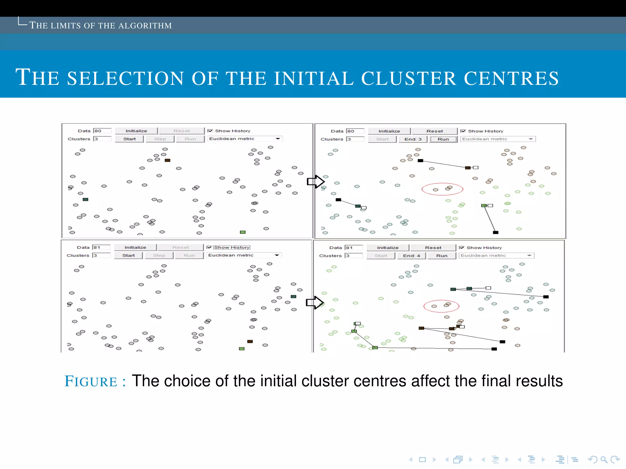
T HE SELECTION OF THE INITIAL CLUSTER CENTRES
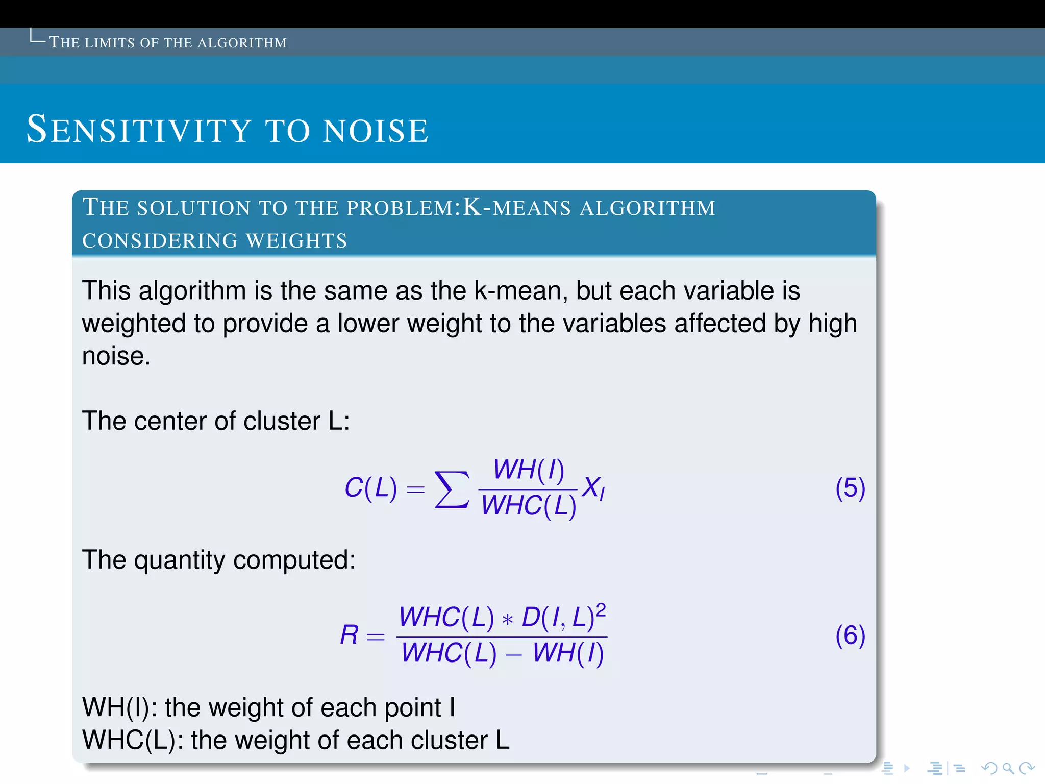
T HE SOLUTION TO THE PROBLEM
Proposed in the article:K sample points are chosen as
the initial cluster centres.
The points are first ordered by their distances to the overall
mean of the sample. Then, for cluster L (L = 1,2, ..., K), the
1 + (L -1) * [M/K]th point is chosen to be its initial cluster
centre (it is guaranteed that no cluster will be empty).
Commonly used:The cluster centers are chosen
randomly.
The algorithm is run several time, then select the set of
cluster with minimum sum of the Squared Error.](https://image.slidesharecdn.com/diapoceline2-121022233756-phpapp01/75/slides-Celine-Beji-55-2048.jpg)


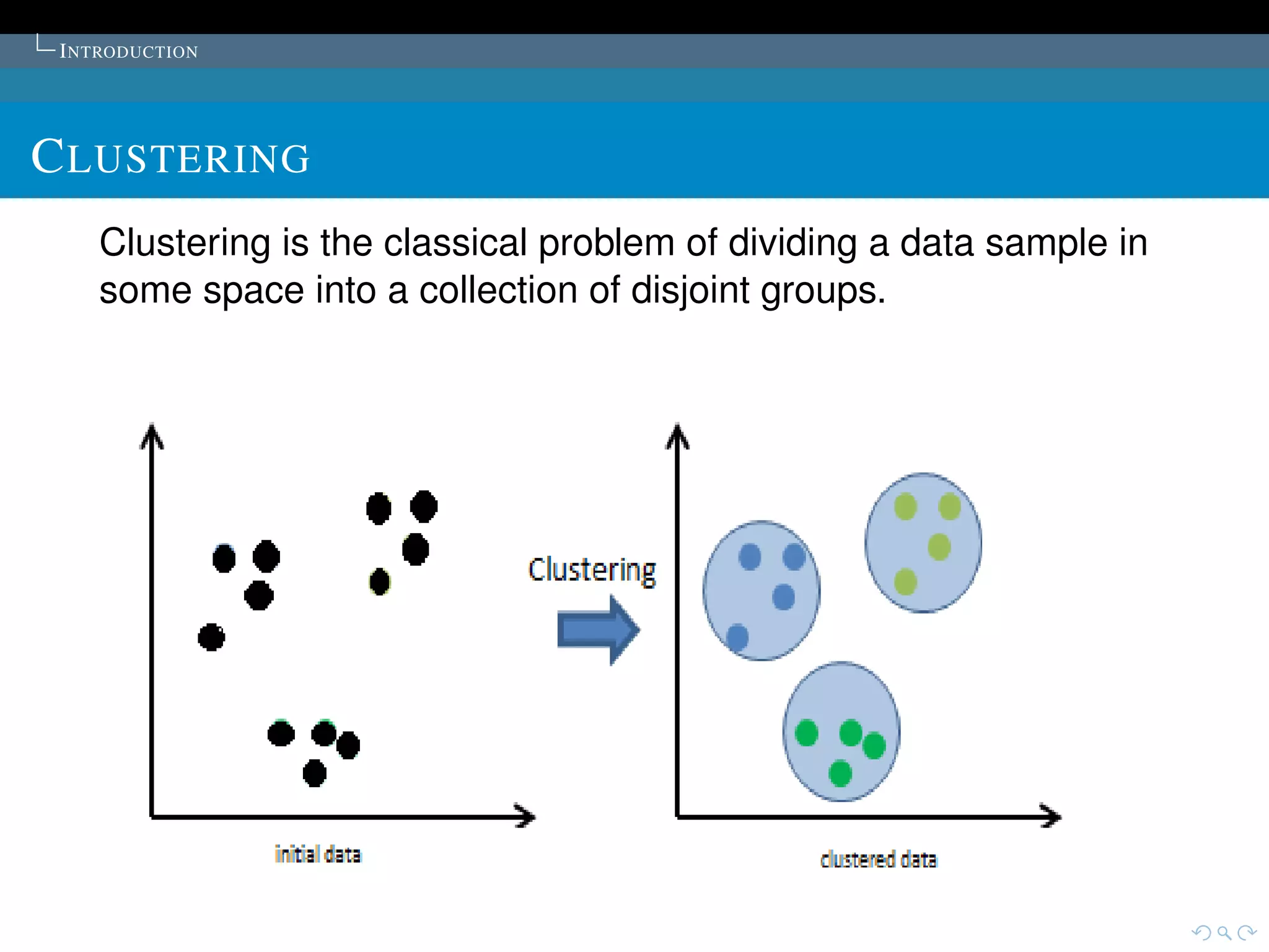
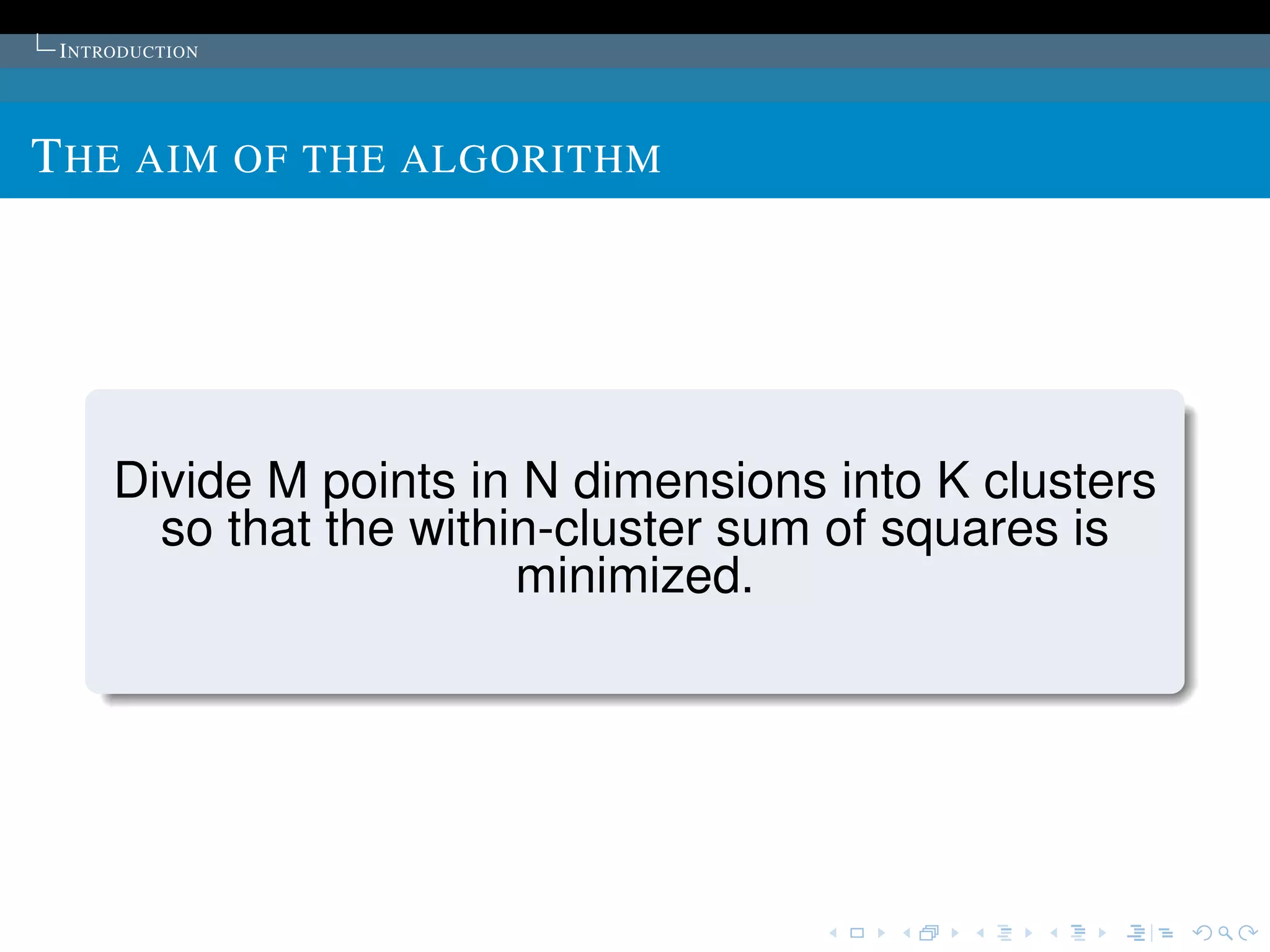
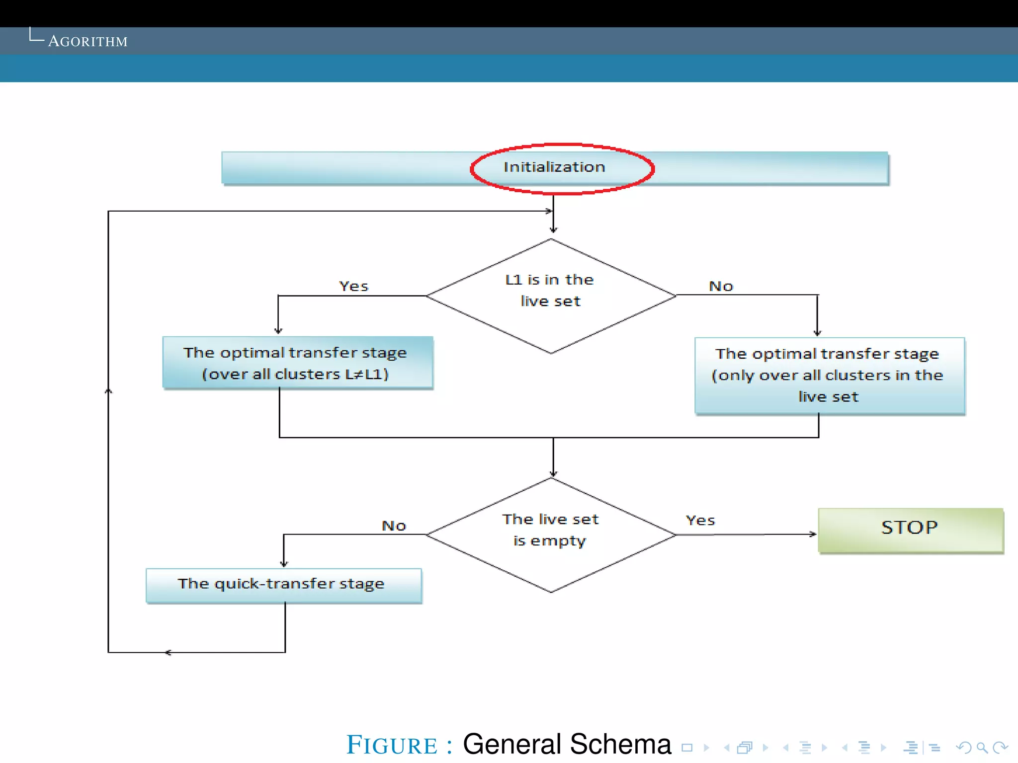
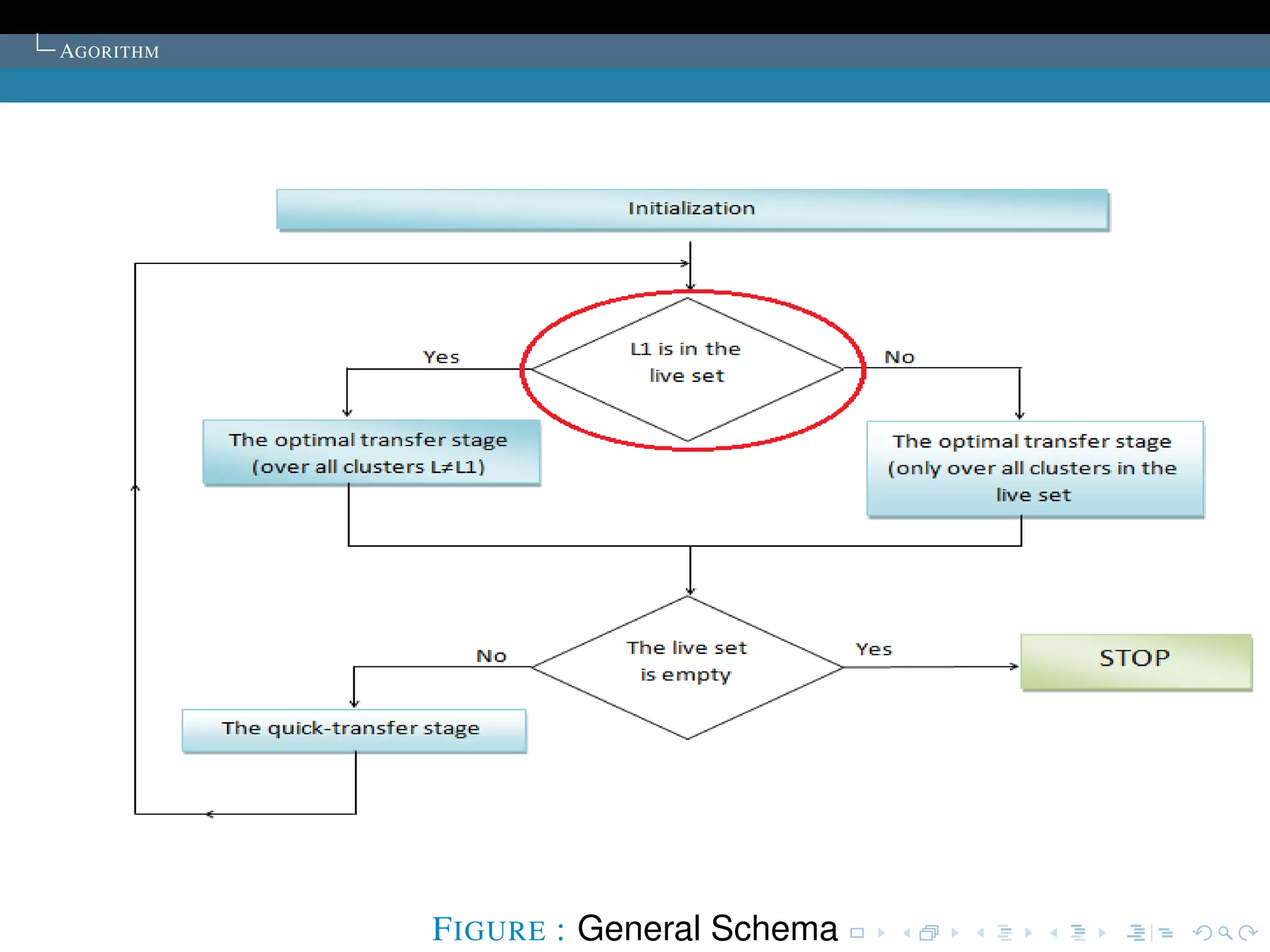
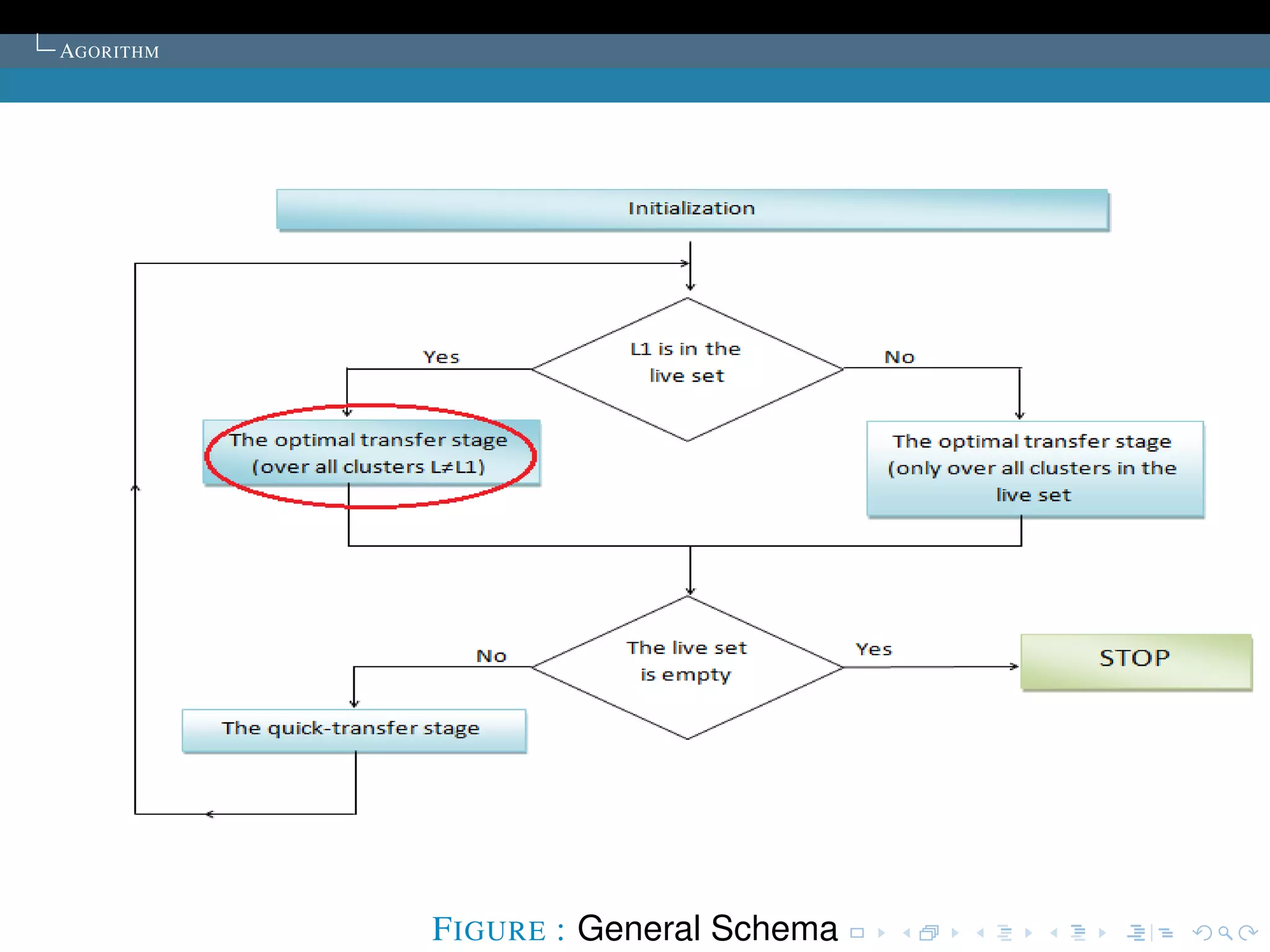
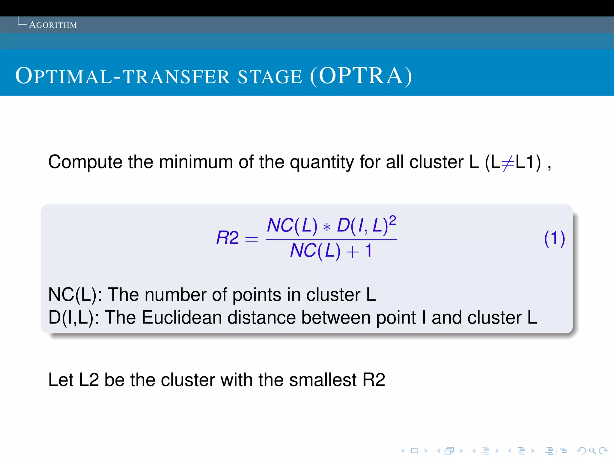
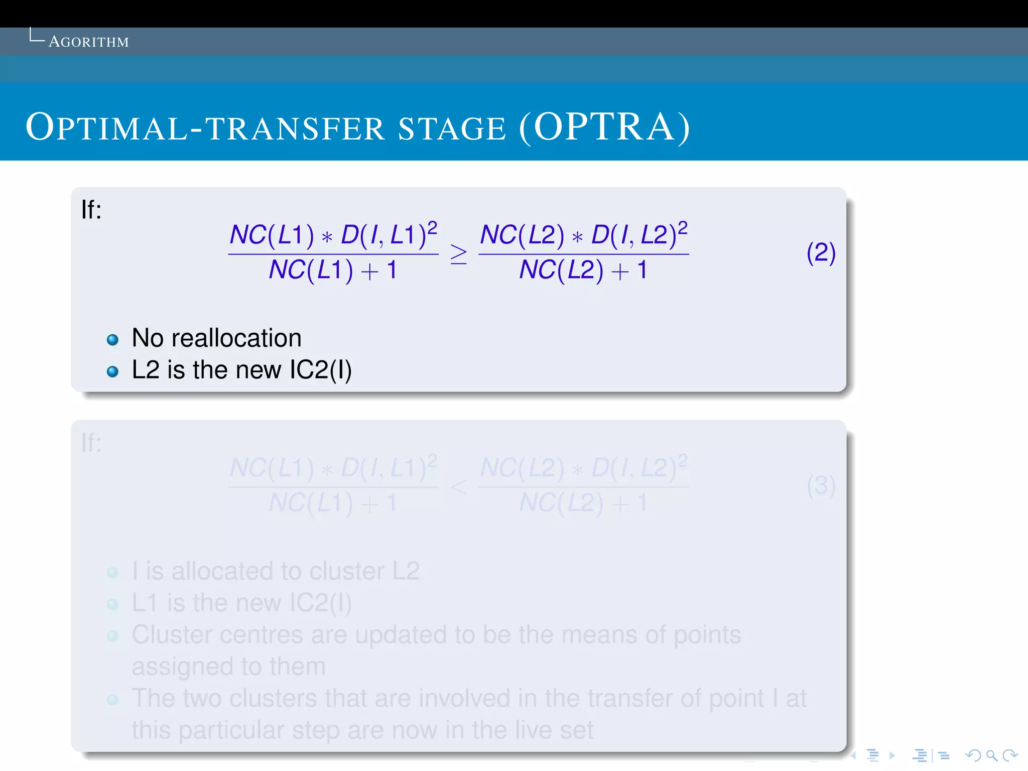
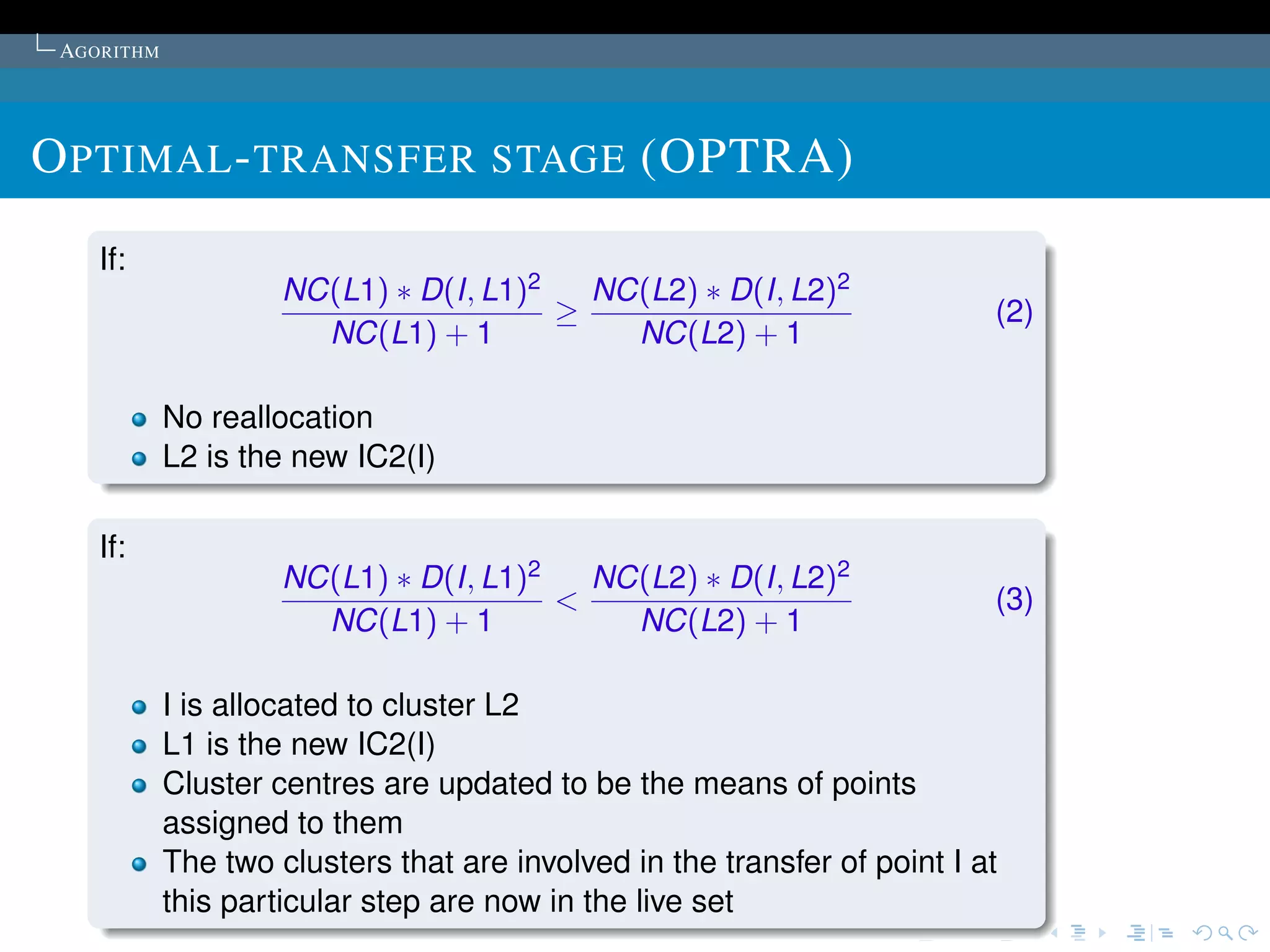
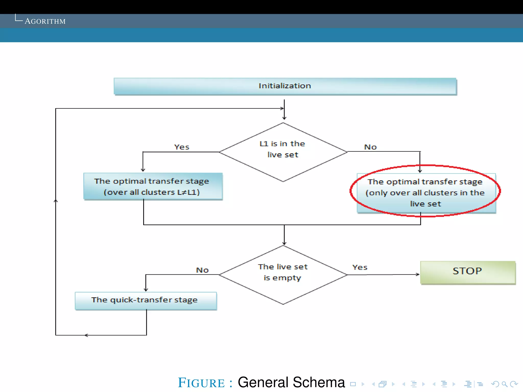
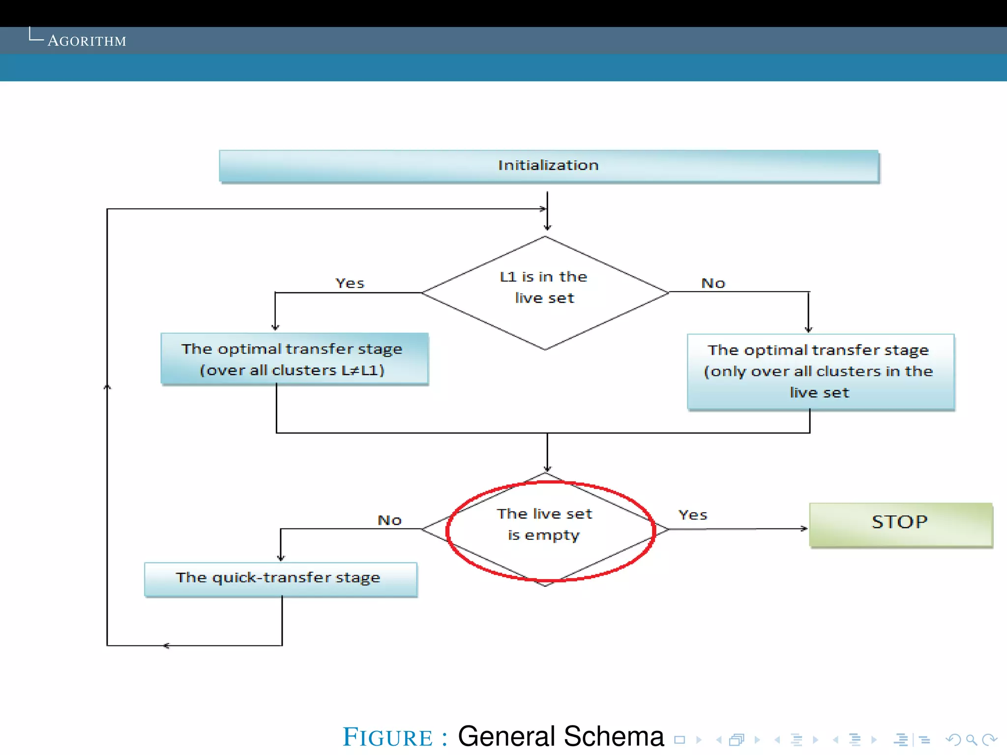
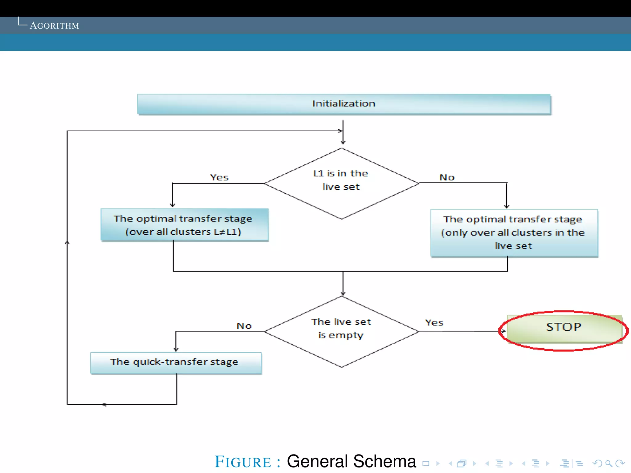
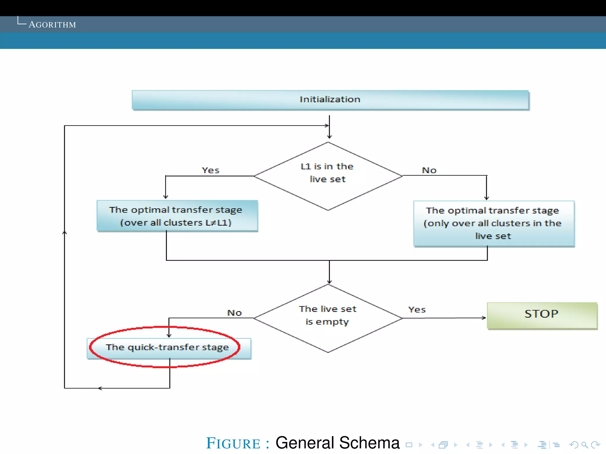
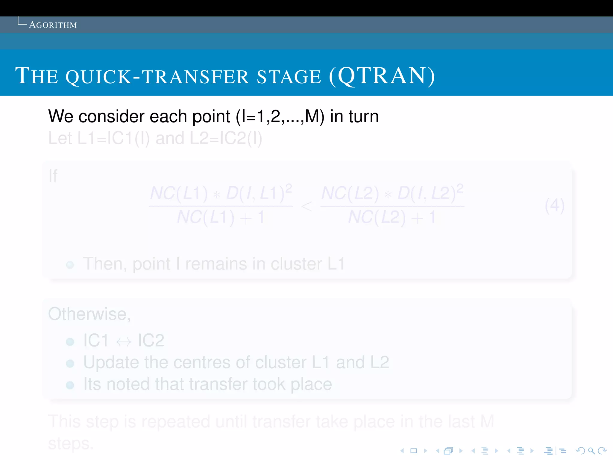
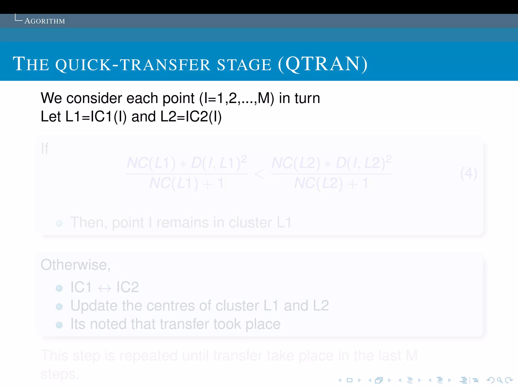
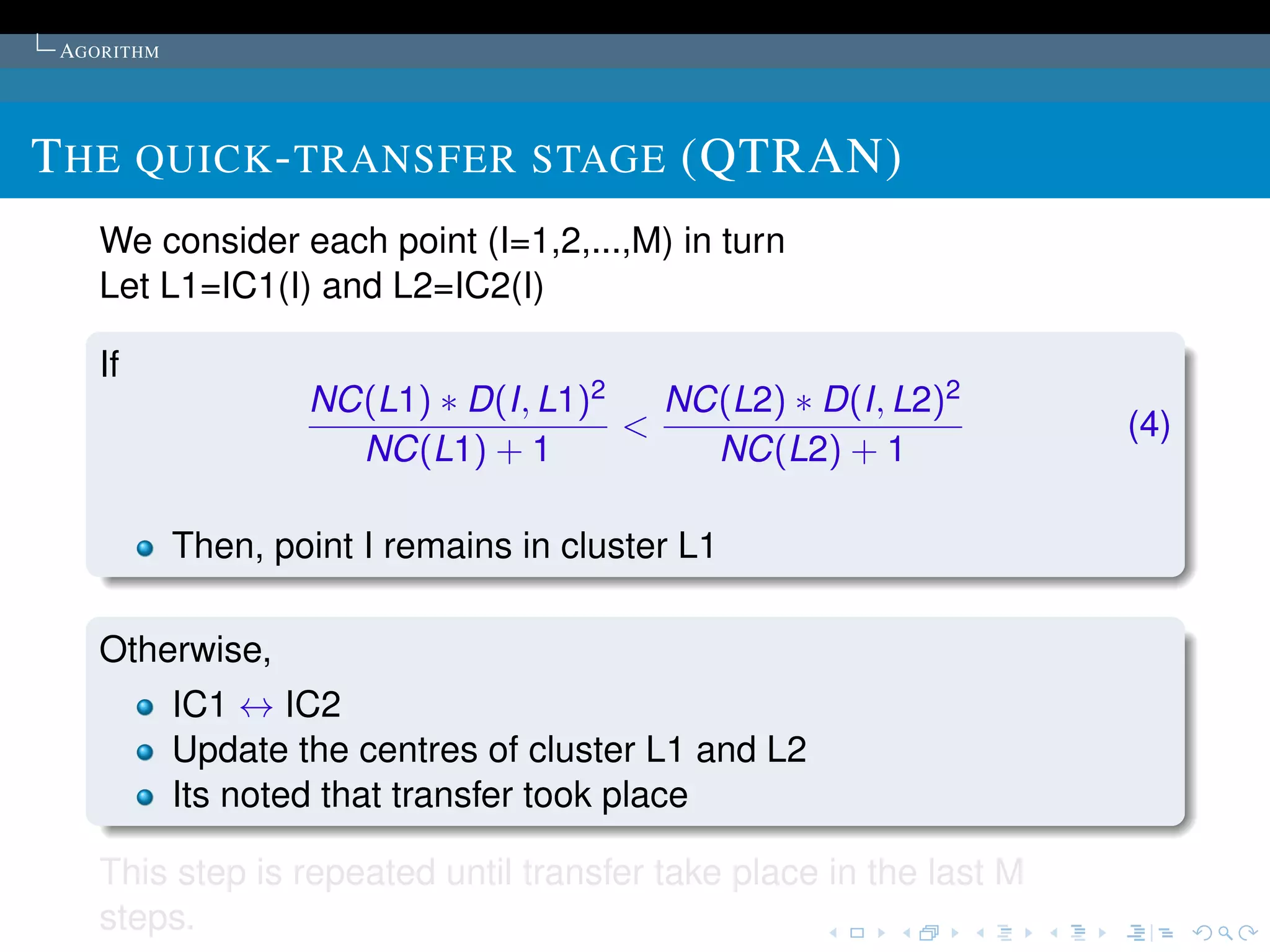
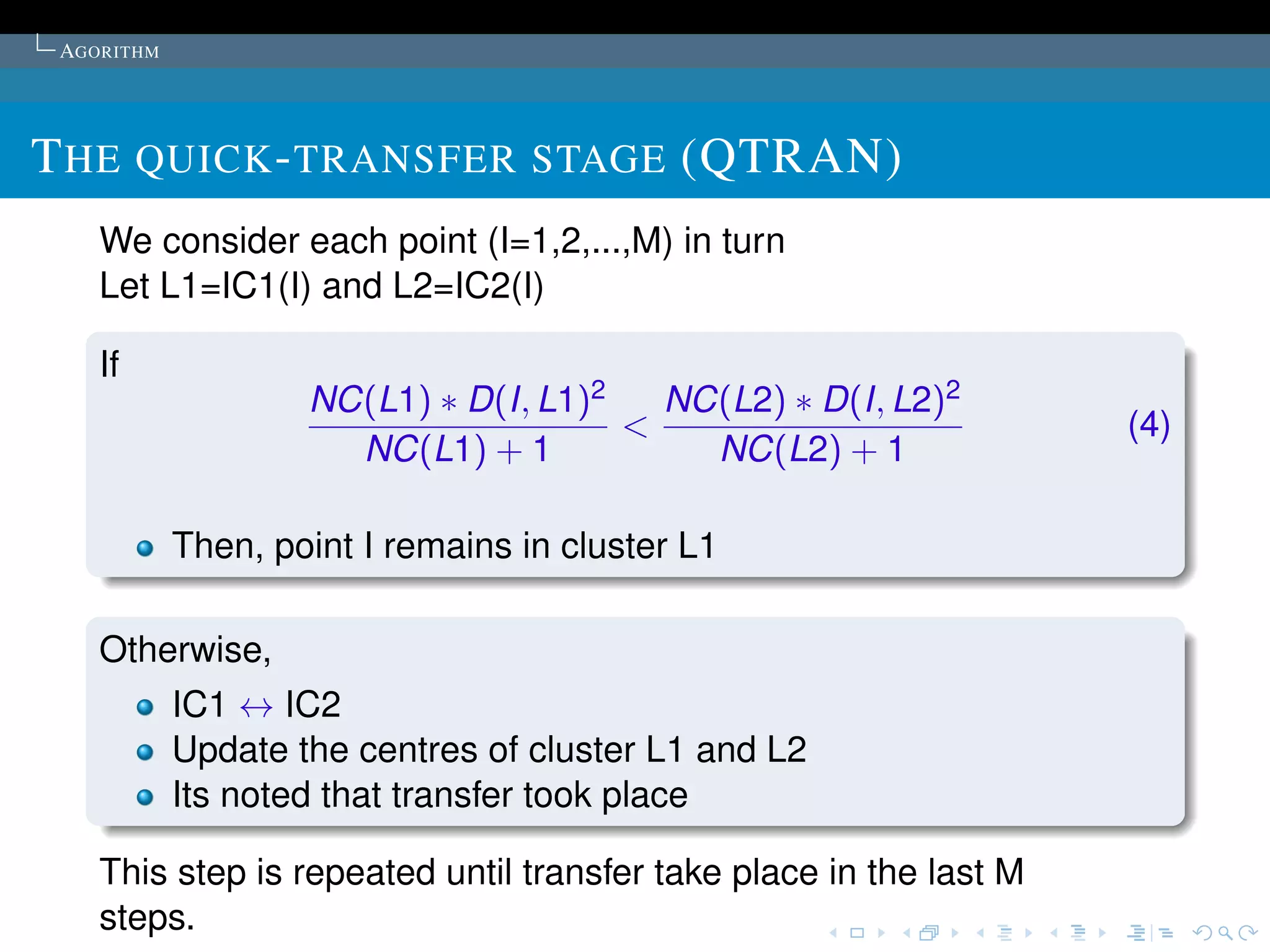
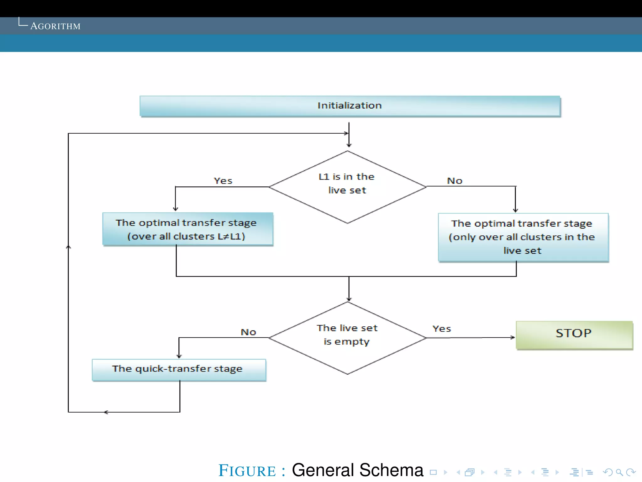
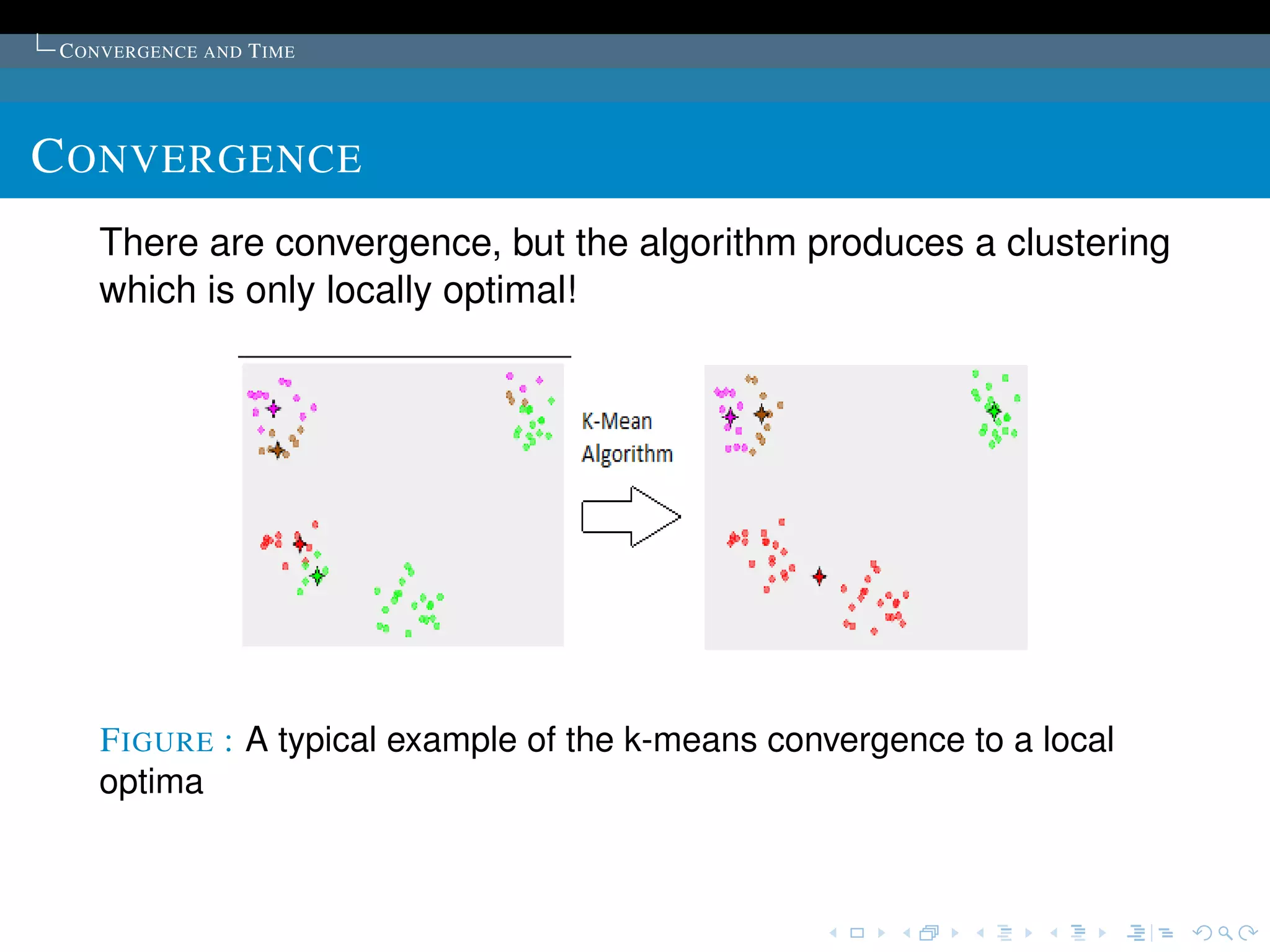
The document describes the k-means clustering algorithm. It introduces clustering and its aim to divide data points into k clusters to minimize within-cluster sums of squares. The algorithm involves initializing cluster centers, then iteratively performing optimal transfers of points between clusters and quick transfers until convergence is reached. Optimal transfers minimize an objective function to determine the best cluster for a point, while quick transfers perform simpler transfers without minimizing the objective.