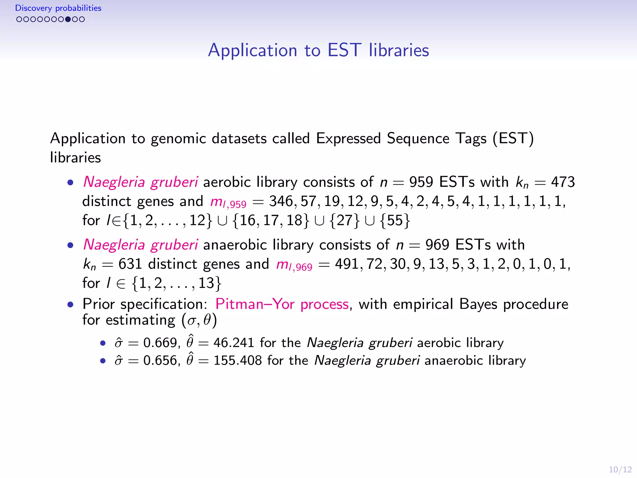
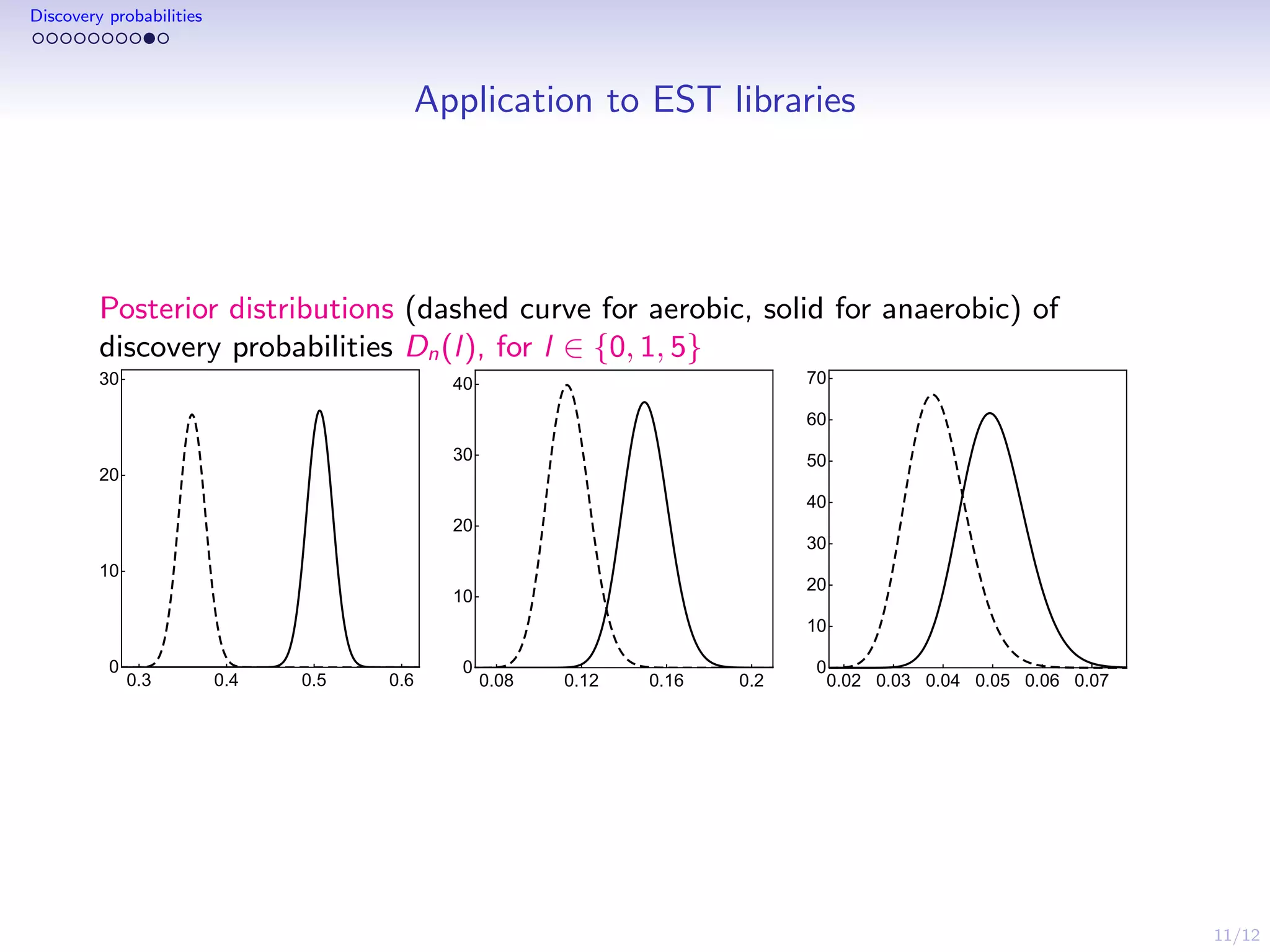
Download as PDF, PPTX
![8/12
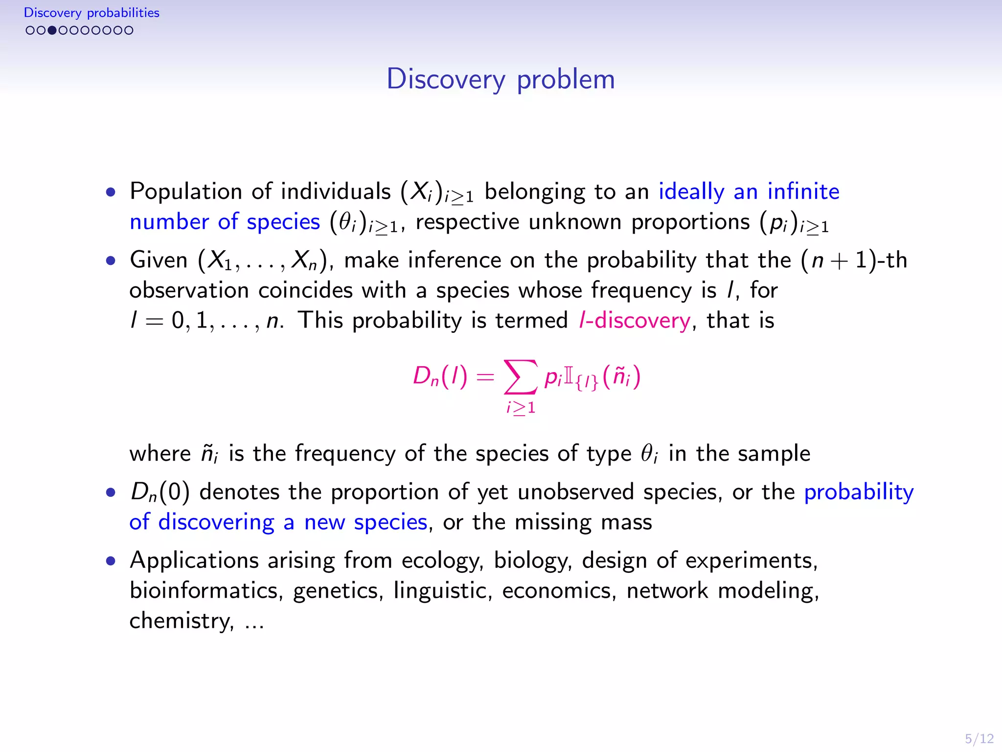
Discovery probabilities
BNP estimators of discovery
Gibbs-type random probability measure P with index σ ∈ (0, 1): it is
characterized by (it induces) a predictive distribution of the form
P[Xn+1 ∈ A | Xn] =
Vn+1,kn+1
Vn,kn
G0(A) +
Vn+1,kn
Vn,kn
kn
i=1
(ni − σ) δX∗
i
(A),
BNP estimator ˆDn(l) of Dn(l) derived from the predictive using sets
A0 = X{X∗
1 , . . . , X∗
Kn
} and Al = {X∗
i : Ni,n = l}
BNP Good Turing
ˆDn(0) = E[Ph(A0) | Xn] =
Vn+1,kn+1
Vn,kn
ˇDn(l) = m1
n
ˆDn(l) = E[Ph(Al ) | Xn] = (l − σ)ml
Vn+1,kn
Vn,kn
ˇDn(l) =
(l+1)ml+1
n](https://image.slidesharecdn.com/statalksjulyanssm-160224162217/75/Species-sampling-models-in-Bayesian-Nonparametrics-8-2048.jpg)

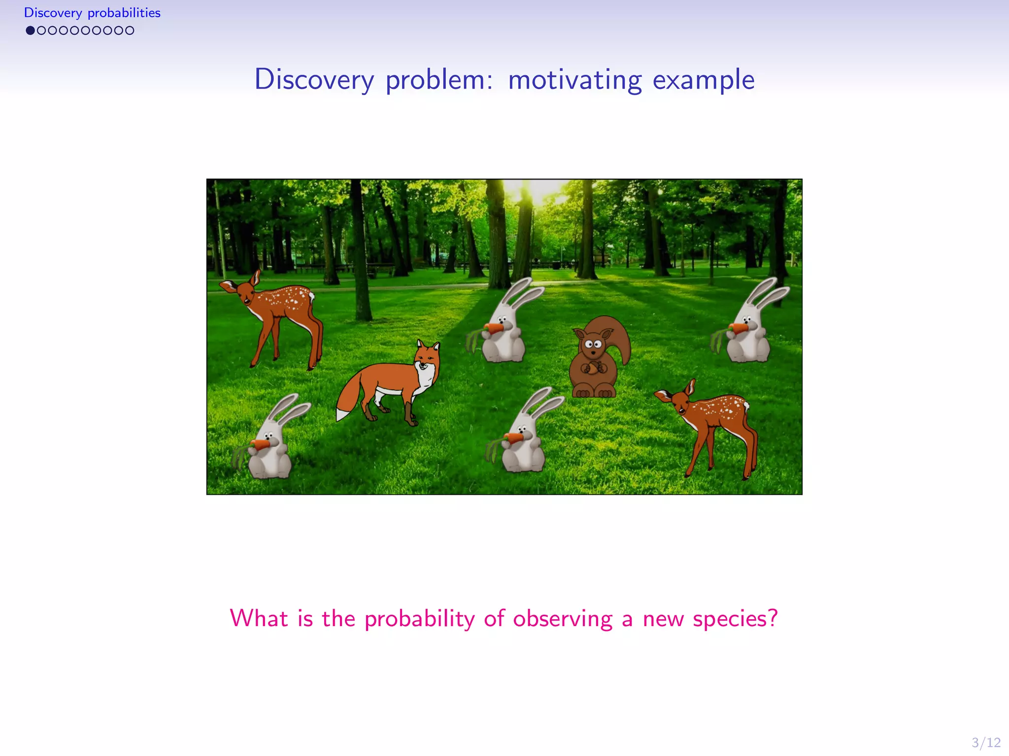
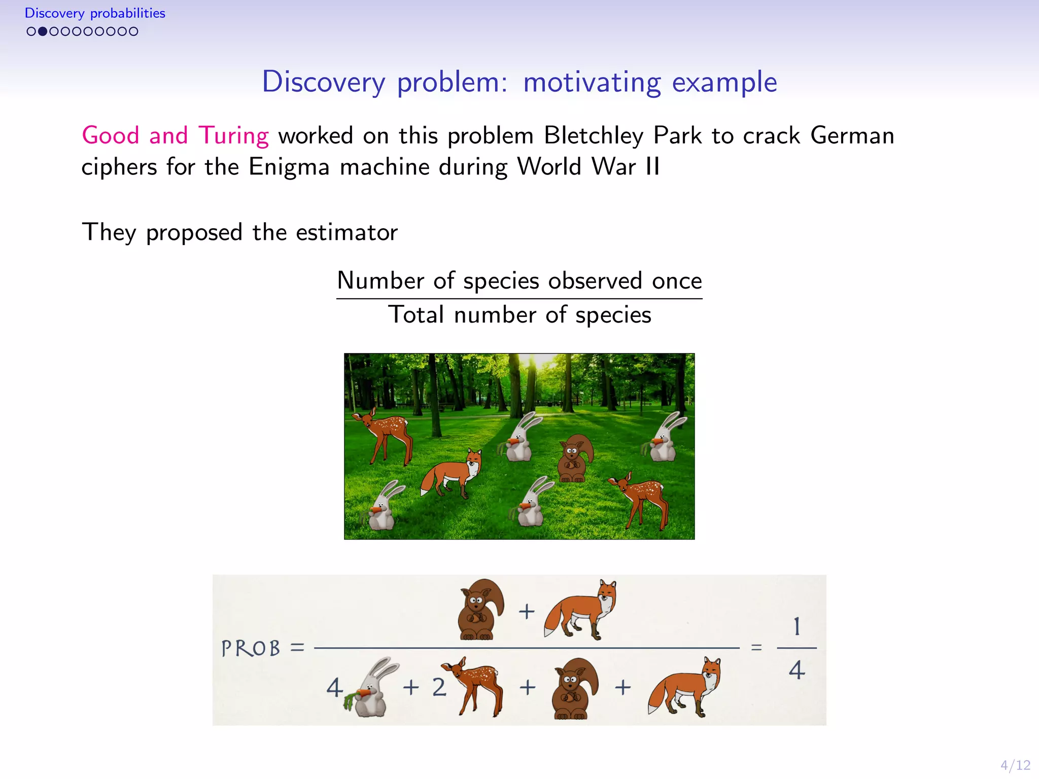
This document discusses species sampling models and discovery probabilities. It introduces the problem of estimating the probability of observing a new species given a sample. Good and Turing proposed an estimator for this during World War II. Bayesian nonparametric models provide an alternative approach by placing a prior on unknown species proportions. The document outlines BNP estimators for discovery probabilities and how credible intervals can be derived. It applies these methods to genomic datasets of expressed sequence tags to estimate discovery probabilities for observing new genes.


![[DSC Europe 25] Danica Soc - The Science Behind Marketing: Experimentation me...](https://cdn.slidesharecdn.com/ss_thumbnails/c0nofsggs9gw5ucmallr-3-251216103155-56bd64d1-thumbnail.jpg?width=640&height=640&fit=bounds)
![[DSC Europe 25] Tatevik Maytesyan - How to actually use AI in marketing: gett...](https://cdn.slidesharecdn.com/ss_thumbnails/tjo626lsqdgfntbgl2mw-4-251216103155-e36cd239-thumbnail.jpg?width=640&height=640&fit=bounds)
![[DSC Europe 25] Hans Kleinsman - The Compliance Gearbox: How Tax Tech Mediate...](https://cdn.slidesharecdn.com/ss_thumbnails/dxdytie1toel0hr90bjs-2-251212103250-174fdbe7-thumbnail.jpg?width=640&height=640&fit=bounds)


![[DSC Europe 25] Jon Dajci - Bridging TradFi and DeFi: Building the Future of ...](https://cdn.slidesharecdn.com/ss_thumbnails/fqmhfvlbqhkihjvqvhmu-7-251211083849-6af7e325-thumbnail.jpg?width=640&height=640&fit=bounds)


![[DSC Europe 25] Nikolay Burlutskiy - Best Practices for Building Enterprise M...](https://cdn.slidesharecdn.com/ss_thumbnails/uirvaiuvq8y1w8hzd9tx-7-251212103249-2619edb4-thumbnail.jpg?width=640&height=640&fit=bounds)


![[DSC Europe 25] Branko Urosevic -Rethinking Financial Talent: Integrating Cod...](https://cdn.slidesharecdn.com/ss_thumbnails/8jjrus8ttko6qj64f58f-3-251212103250-642c6374-thumbnail.jpg?width=640&height=640&fit=bounds)
![[DSC Europe 25] Bassam Maharmeh - Artificial Intelligence: Opportunities and ...](https://cdn.slidesharecdn.com/ss_thumbnails/thhfmr2fqpawzj7hsjpg-5-251211083048-2c23204f-thumbnail.jpg?width=640&height=640&fit=bounds)
![[DSC Europe 25] Katherine Forrest - AI NOW: Understanding the Velocity of Cha...](https://cdn.slidesharecdn.com/ss_thumbnails/wvvbruqfrci0sfq9xwgb-4-251212104007-e5ad1987-thumbnail.jpg?width=640&height=640&fit=bounds)