This document is the preface to a book on fuzzy control and identification. It provides background on the author's interest and experience in fuzzy systems, as well as the motivation for writing the book. The author aims to present an introductory exposure to the principal uses of fuzzy logic for identification and control. The book covers topics not fully addressed in other texts, at a level appropriate for senior undergraduates and first-year graduate students. It seeks to bridge material from introductory and advanced control courses.

1. FUZZY CONTROL AND
IDENTIFICATION
JOHN H. LILLY
JOHN WILEY & SONS, INC.

3. FUZZY CONTROL AND
IDENTIFICATION

5. FUZZY CONTROL AND
IDENTIFICATION
JOHN H. LILLY
JOHN WILEY & SONS, INC.

6. Copyright © 2010 by John Wiley & Sons, Inc. All rights reserved
Published by John Wiley & Sons, Inc., Hoboken, New Jersey
Published simultaneously in Canada
No part of this publication may be reproduced, stored in a retrieval system, or transmitted in any form
or by any means, electronic, mechanical, photocopying, recording, scanning, or otherwise, except as
permitted under Section 107 or 108 of the 1976 United States Copyright Act, without either the prior
written permission of the Publisher, or authorization through payment of the appropriate per-copy fee
to the Copyright Clearance Center, Inc., 222 Rosewood Drive, Danvers, MA 01923, (978) 750-8400,
fax (978) 750-4470, or on the web at www.copyright.com. Requests to the Publisher for permission
should be addressed to the Permissions Department, John Wiley & Sons, Inc., 111 River Street,
Hoboken, NJ 07030, (201) 748-6011, fax (201) 748-6008, or online at http://www.wiley.com/go/
permission.
Limit of Liability/Disclaimer of Warranty: While the publisher and author have used their best efforts
in preparing this book, they make no representations or warranties with respect to the accuracy or
completeness of the contents of this book and specifically disclaim any implied warranties of
merchantability or fitness for a particular purpose. No warranty may be created or extended by sales
representatives or written sales materials. The advice and strategies contained herein may not be
suitable for your situation. You should consult with a professional where appropriate. Neither the
publisher nor author shall be liable for any loss of profit or any other commercial damages, including
but not limited to special, incidental, consequential, or other damages.
For general information on our other products and services or for technical support, please contact our
Customer Care Department within the United States at (800) 762-2974, outside the United States at
(317) 572-3993 or fax (317) 572-4002.
Wiley also publishes its books in a variety of electronic formats. Some content that appears in print
may not be available in electronic formats. For more information about Wiley products, visit our web
site at www.wiley.com.
Library of Congress Cataloging-in-Publication Data:
Lilly, John H., 1949–
Fuzzy control and identification / John H. Lilly.
p. cm.
ISBN 978-0-470-54277-4 (cloth)
1. Fuzzy automata. 2. System identification. 3. Automatic control–Mathematics. I. Title.
TJ213.L438 2010
629.8–dc22
2010007956
Printed in the United States of America
10 9 8 7 6 5 4 3 2 1

7. For Faith, Jack, and Sarah

9. PREFACE xi
CHAPTER 1 INTRODUCTION 1
1.1 Fuzzy Systems 1
1.2 Expert Knowledge 3
1.3 When and When Not to Use Fuzzy Control 3
1.4 Control 4
1.5 Interconnection of Several Subsystems 6
1.6 Identification and Adaptive Control 8
1.7 Summary 9
Exercises 10
CHAPTER 2 BASIC CONCEPTS OF FUZZY SETS 11
2.1 Fuzzy Sets 11
2.2 Useful Concepts for Fuzzy Sets 15
2.3 Some Set Theoretic and Logical Operations on Fuzzy Sets 16
2.4 Example 18
2.5 Singleton Fuzzy Sets 22
2.6 Summary 23
Exercises 24
CHAPTER 3 MAMDANI FUZZY SYSTEMS 27
3.1 If-Then Rules and Rule Base 27
3.2 Fuzzy Systems 29
3.3 Fuzzification 29
3.4 Inference 30
3.5 Defuzzification 30
3.5.1 Center of Gravity (COG) Defuzzification 31
3.5.2 Center Average (CA) Defuzzification 31
3.6 Example: Fuzzy System for Wind Chill 31
3.6.1 Wind Chill Calculation, Minimum T-Norm, COG Defuzzification 35
3.6.2 Wind Chill Calculation, Minimum T-Norm, CA Defuzzification 38
3.6.3 Wind Chill Calculation, Product T-Norm, COG Defuzzification 38
3.6.4 Wind Chill Calculation, Product T-Norm, CA Defuzzification 41
3.6.5 Wind Chill Calculation, Singleton Output Fuzzy Sets, Product T-Norm,
CA Defuzzification 41
3.7 Summary 42
Exercises 43
TABLE OF CONTENTS
vii

10. viii TABLE OF CONTENTS
CHAPTER 4 FUZZY CONTROL WITH MAMDANI SYSTEMS 46
4.1 Tracking Control with a Mamdani Fuzzy Cascade Compensator 46
4.1.1 Initial Fuzzy Compensator Design: Ball and Beam Plant 47
4.1.2 Rule Base Determination: Ball and Beam Plant 50
4.1.3 Inference: Ball and Beam Plant 52
4.1.4 Defuzzification: Ball and Beam Plant 53
4.2 Tuning for Improved Performance by Adjusting Scaling Gains 53
4.3 Effect of Input Membership Function Shapes 56
4.4 Conversion of PID Controllers into Fuzzy Controllers 59
4.4.1 Redesign for Increased Robustness 64
4.5 Incremental Fuzzy Control 66
4.6 Summary 69
Exercises 69
CHAPTER 5 MODELING AND CONTROL METHODS USEFUL FOR
FUZZY CONTROL 71
5.1 Continuous-Time Model Forms 71
5.1.1 Nonlinear Time-Invariant Continuous-Time State-Space Models 71
5.1.2 Linear Time-Invariant Continuous-Time State-Space Models 74
5.2 Model Forms for Discrete-Time Systems 75
5.2.1 Input–Output Difference Equation Model for Linear Discrete-Time
Systems 76
5.2.2 Linear Time-Invariant Discrete-Time State-Space Models 76
5.3 Some Conventional Control Methods Useful in Fuzzy Control 78
5.3.1 Pole Placement Control 79
5.3.2 Tracking Control 81
5.3.3 Model Reference Control 82
5.3.4 Feedback Linearization 84
5.4 Summary 85
Exercises 86
CHAPTER 6 TAKAGI–SUGENO FUZZY SYSTEMS 88
6.1 Takagi–Sugeno Fuzzy Systems as Interpolators between Memoryless Functions 88
6.2 Takagi–Sugeno Fuzzy Systems as Interpolators between Continuous-Time Linear
State-Space Dynamic Systems 92
6.3 Takagi–Sugeno Fuzzy Systems as Interpolators between Discrete-Time Linear
State-Space Dynamic Systems 95
6.4 Takagi–Sugeno Fuzzy Systems as Interpolators between Discrete-Time
Dynamic Systems described by Input–Output Difference Equations 98
6.5 Summary 101
Exercises 101
CHAPTER 7 PARALLEL DISTRIBUTED CONTROL WITH
TAKAGI–SUGENO FUZZY SYSTEMS 106
7.1 Continuous-Time Systems 106
7.2 Discrete-Time Systems 109
7.3 Parallel Distributed Tracking Control 112
7.4 Parallel Distributed Model Reference Control 116
7.5 Summary 118
Exercises 119

11. TABLE OF CONTENTS ix
CHAPTER 8 ESTIMATION OF STATIC NONLINEAR FUNCTIONS FROM DATA 121
8.1 Least-Squares Estimation 121
8.1.1 Batch Least Squares 122
8.1.2 Recursive Least Squares 123
8.2 Batch Least-Squares Fuzzy Estimation in Mamdani Form 124
8.3 Recursive Least-Squares Fuzzy Estimation in Mamdani Form 132
8.4 Least-Squares Fuzzy Estimation in Takagi–Sugeno Form 135
8.5 Gradient Fuzzy Estimation in Mamdani Form 136
8.6 Gradient Fuzzy Estimation in Takagi–Sugeno Form 145
8.7 Summary 146
Exercises 147
CHAPTER 9 MODELING OF DYNAMIC PLANTS AS FUZZY SYSTEMS 149
9.1 Modeling Known Plants as Takagi–Sugeno Fuzzy Systems 149
9.2 Identification in Input–Output Difference Equation Form 154
9.2.1 Batch Least-Squares Identification in Difference Equation Form 154
9.2.2 Recursive Least-Squares Identification in Input–Output Difference Equation
Form 159
9.2.3 Gradient Identification in Input–Output Difference Equation Form 160
9.3 Identification in Companion Form 163
9.3.1 Least-Squares Identification in Companion Form 163
9.3.2 Gradient Identification in Companion Form 165
9.4 Summary 167
Exercises 168
CHAPTER 10 ADAPTIVE FUZZY CONTROL 169
10.1 Direct Adaptive Fuzzy Tracking Control 170
10.2 Direct Adaptive Fuzzy Model Reference Control 173
10.3 Indirect Adaptive Fuzzy Tracking Control 175
10.4 Indirect Adaptive Fuzzy Model Reference Control 179
10.5 Adaptive Feedback Linearization Control 184
10.6 Summary 187
Exercises 188
REFERENCES 190
APPENDIX COMPUTER PROGRAMS 192
INDEX 229

13. xi
In 1982, when I obtained my Ph.D. specializing in adaptive control (the nonfuzzy
kind), fuzzy control had not been explored to a very great extent as a research area.
There had been only a handful of papers (probably <100) published on the subject
up to that time, and some of us “serious researchers” did not take fuzzy seriously
as a control method. Since then, of course, the number of papers and books written
on some application of fuzzy sytstems has grown to tens of thousands, and many of
us “serious researchers,” after realizing the potential of the fuzzy approach, have
partially or completely redirected our research efforts to some aspect or application
of fuzzy identification, classification, or control.
Roughly 10 years after graduating, I started reading anything I could find on
the subjects of fuzzy identification and control, culminating in the creation of a
graduate-level course on the subject at the University of Louisville. This book is an
outgrowth of lectures I presented in this course over the past 10 years, plus some
new material that I have not presented yet, but probably will at some point.
I wrote this book to present an introductory-level exposure to two of the prin-
cipal uses for fuzzy logic: identification and control. This book was written to
include topics that I deem important to the subject, but that I could not find all
together in any one text. I kept finding myself borrowing material from several
sources to teach my course, which is suboptimal for teacher and student alike. In
addition, I found that many texts, although excellent, were written on too high a
level to be useful as introductory texts. (It is ironic that a subject ridiculed by many
as “too easy” quickly becomes so complex as to turn most people away once the
basics are covered.) Consequently, I wrote this book, which includes subjects that I
think important at hopefully not such a high level as to “blow away” most
students.
The book is intended for seniors and first-year graduate students. Some back-
ground in control is helpful, but many topics covered in introductory controls courses
are of little use here, such as gain and phase margins, root locus, Bode and Nyquist
plots, transient and steady-state response, and so on. On the other hand, some of the
subjects addressed in this book, such as tracking, model reference, adaptive identi-
fication and control, are only covered in advanced-level controls courses. This is in
part what makes this subject difficult to teach.
The most helpful preparation would be some understanding of continuous- and
discrete-time dynamic systems, and an appreciation of the basic aims and methods
of control (i.e., stabilization, tracking, and model reference control). There is little
PREFACE

14. xii PREFACE
in the way of advanced mathematics beyond differential and difference equations,
transfer functions, and linear algebra required to read and understand this book.
The subjects of fuzzy identification and control are quite heavy in computer
programming. In order to implement or simulate fuzzy systems, it is almost unavoid-
able to write computer programs, so it is assumed that the reader is comfortable with
at least basic computer programming and computer simulation of dynamic systems.
In this book, Matlab is used exclusively for simulations due to its ease of program-
ming matrix manipulations and plotting. I have not relied on any Matlab “canned”
programs (e.g., the Matlab differential equation solvers ode23, ode45, etc.) or tool-
boxes (e.g., the Fuzzy Logic Toolbox). One exception is the use of the LMI Control
Toolbox used in Chapter 7 to solve a linear matrix inequality. The avoidance of these
very powerful specialized tools that Matlab provides was done to give a measure of
transparency in the example programs provided in the Appendix, and also because
whatever computer language is used to implement these controllers may not (in fact,
probably will not) have them.
ARRANGEMENT OF THIS BOOK
The arrangement of this book may seem strange to some. Chapter 5, which presents
some well-known nonfuzzy modeling and control methods, may look out of place
in the middle of the other chapters, which have to do with only fuzzy topics. It was
suggested to me that the material in Chapter 5 either be placed in an introductory
chapter or relegated to an appendix. However, I felt there is good reason to place it
where it is.
Chapters 2–4 cover basic concepts of fuzzy logic, fuzzy sets, fuzzy systems,
and control with Mamdani fuzzy systems. All controllers presented in Chapter 4 are
designed on the basis of “expert knowledge.” Their design is not based on any
mathematical model of the system they control, nor do they use any formal control
method (pole placement, tracking, etc.). Therefore, there is no need to study math-
ematical modeling or control methods to utilize anything through Chapter 4.
On the other hand, Chapters 6 and 7 introduce Takagi–Sugeno (T–S) fuzzy
systems, which do necessitate the utilization of a plant model along with choice of
some formal control methodology. Thus, the introduction of some standard modeling
and control techniques seemed well placed between the Mamdani and T–S develop-
ments. I felt that placing this material in either an introductory chapter or an appendix
would reduce its chances of being read. At any rate, the chapters are as follows.
Chapter 1 is an introduction to fuzzy logic, fuzzy control, and adaptive fuzzy
control. We introduce the concept of expert knowledge, which is the basis for much
of fuzzy control. We talk briefly about when fuzzy methods may be justified, when
they may not, and why. We discuss the plants used in the examples to illustrate
various principles taught in this book. Also included in Chapter 1 are brief
descriptions of the identification and control problems. Finally, these are combined
to discuss the concept of adaptive fuzzy control.
Chapter 2 covers basic concepts of fuzzy sets, such as membership functions,
universe of discourse, linguistic variables, linguistic values, support, α-cut, and

15. PREFACE xiii
convexity. We also discuss some set theoretic and logical operations on fuzzy sets,
such as fuzzy subset, fuzzy complement, fuzzy intersection, and fuzzy Cartesian
product.
Chapter 3 introduces Mandani fuzzy systems, which were historically the first
type of fuzzy system used for control. We discuss the various processes that make
up fuzzy systems, including fuzzification, inference, defuzzification, and rule base.
We discuss the two most common types of defuzzification: center of gravity and
center average. In this chapter, we also introduce the concept of the input–output
characteristic of a fuzzy controller. Finally, we introduce the singleton fuzzy set,
which is used in all subsequent fuzzy identifiers and controllers in this book.
Chapter 4 discusses closed-loop fuzzy control with Mamdani fuzzy systems.
It is shown how an effective controller can be designed for many complex nonlinear
systems using only common sense. We discuss how the controller can be tuned for
improved performance by scaling universes of discourse. We also discuss how fuzzy
controllers can be redesigned (again on the basis of common sense) to increase
robustness. Chapter 4 includes a method of converting a nonfuzzy proportional-
integral-derivative (PID) controller into a fuzzy controller for the purpose of rede-
signing it to increase robustness. This chapter also includes an introduction to
incremental fuzzy control.
Chapter 5 is nonfuzzy. It contains a summary of some common modeling
and control techniques that will be used in the rest of the book. It is shown how
continuous-time nonlinear systems, which most real-world systems are, can be
modeled as fuzzy systems in several forms (continuous-time feedback linearizable
form, continuous- and discrete-time linear state-space form, and discrete-time input–
output difference equation form). All of these forms are used later in the book. Also
included in Chapter 5 are some conventional control methods used in fuzzy control,
such as pole placement control, tracking control, model reference control, and
feedback linearization. Again, these are introduced because they are used later in
the book.
Chapter 6 introduces T–S fuzzy systems as interpolators between memoryless
functions, continuous- and discrete-time dynamic systems described in state-space
form, and discrete time linear input–output dynamic systems.
Chapter 7 introduces parallel distributed control with T–S fuzzy systems. We
introduce the concept of linear matrix inequalities, by which stability can be proved
for closed-loop systems involving fuzzy controllers. We discuss how fuzzy tracking
and model reference control can be realized for nonlinear systems using parallel
distributed controllers.
Chapter 8 discusses the estimation of static nonlinear functions from data using
the batch least squares, recursive least squares, and gradient methods. The gradient
parameter update equations, similar to backpropagation in neural networks, are
derived. We address the importance of choice of input data, as well as model valida-
tion for these methods.
Chapter 9 uses the principles discussed in Chapter 8 to obtain T–S fuzzy
models of dynamic plants for the purpose of using these for closed-loop control.
The chapter begins by giving a method of modeling time-invariant nonlinear systems
with known mathematical models, with T–S fuzzy systems. The remainder of the

16. xiv PREFACE
chapter is concerned with identification from data of nonlinear continuous time
systems as T–S fuzzy systems in either feedback linearizeable or input–output dif-
ference equation form.
Chapter 10 uses the principles given in Chapter 9 to develop direct and indirect
adaptive fuzzy controllers. These methods are applied to several different systems
including a motor-driven robot arm, a ball-and-beam system, and a gantry.
WHAT IS NOT COVERED IN THIS BOOK
A thorough presentation of the topics covered in this book would be quite involved
technically and would include a lot of complicated notation. While this is certainly
valuable and even indispensable to one wanting to be fully versed in fuzzy control
and identification, I have tried to streamline things somewhat in this introductory
exposition of the subject by omitting some topics. Specifically, the following topics,
which are well known to fuzzy practitioners, are not covered here.
1. Fuzzification Methods Other Than Singleton Fuzzification
Fuzzification is the method by which measured quantities from real-world
systems are converted into fuzzy sets. There are many methods of fuzzifica-
tion, depending on how the measured quantities are to be interpreted. The most
straightforward fuzzification philosophy is singleton fuzzification, in which the
measured quantities are simply taken to be exact as measured. Since most
fuzzification in practice is of the singleton type, this is the only fuzzification
strategy considered here.
2. Nonsingleton Membership Function Shapes Other Than Triangles and
Gaussians
In general, the membership function characterizing a fuzzy set
should accurately reflect membership in the set. Thus the choice of shapes is
virtually unlimited. In practice, however, only a few membership shapes tend
to be used much. Of these, we have chosen triangular and Gaussian shapes
(triangular because of the possibility of partitions of unity, and Gaussian
because of their usefulness in fuzzy identifiers and adaptive controllers).
3. Defuzzification Methods Other Than Center of Gravity and Center Average
Defuzzification is the method by which fuzzy sets are converted into crisp
numbers to be delivered to the outside world. There are numerous defuzzifica-
tion strategies, but we have chosen to present only the two most common ones:
center of gravity and center average defuzzification.
4. Overall Implied Fuzzy Sets for Defuzzification
Overall implied fuzzy sets are not covered for defuzzification here in favor of
the more straightforward individual implied fuzzy sets.
5. Universal Approximation Property of Fuzzy Systems
The universal approximation property of fuzzy systems states that any function
can be approximated by a fuzzy system to arbitrary accuracy. It is important
in that it justifies the use of fuzzy identifiers for nonlinear systems. However,

17. PREFACE xv
it can be found in many references, and seemed slightly off-topic for the pur-
poses of this book. Therefore, it is omitted.
6. Identification Methods Other Than Least Squares and Gradient
We concentrate on batch and recursive least squares (RLS) and gradient
methods and omit other methods, such as orthogonal projection, least-mean
squares, clustering, and learning from examples. Also omitted are methods
that add momentum to identification techniques.
ACKNOWLEDGMENTS
I would like to acknowledge the help of several people who directly or indirectly
influenced me in the writing of this book. First, I have learned much from my Ph.D.
students Jerry Branson, Liang Yang, and Jie Liu, all of whom expanded my thinking
in fuzzy control in various ways. Second, my colleague Jacek Zurada, who himself
is the author of several excellent books on neural networks and computational intel-
ligence, has helped me immeasurably in my career and has given me excellent advice
and inspiration. I am grateful to my own Ph.D. advisor, Prof. Mark Balas, for giving
me an appreciation of mathematics and rigor in engineering. Finally, I would like
to thank Prof. Chi-Tsong Chen, who is the author of numerous excellent textbooks
in control, linear systems, and signals, for indirectly inspiring me to write this book.
His inspiration came several decades ago when I taught at SUNY Stony Brook, but
I have never forgotten it.

19. 1
Fuzzy Control and Identification, By John H. Lilly
Copyright © 2010 John Wiley & Sons, Inc.
The English-language thesaurus has the following synonyms for “fuzzy”: ill-defined,
indefinite, indistinct, murky, obscure, unclear, vague, and so on. These are words
that English-speaking people associate with fuzzy logic, fuzzy control, fuzzy iden-
tification, and fuzzy systems. They are not words that anyone would want associated
with engineering systems, on which may depend large sums of money, or even
worse, peoples’ lives. It is unfortunate that the word “fuzzy” was chosen to describe
the type of identification and control described in this book. Japanese has no such
negative connotations associated with the word “fuzzy,” hence systems utilizing
fuzzy identification and control are far more prevalent in Japan than in English-
speaking countries.
Fuzzy logic, as will be seen in Chapter 3, is modeled on the human reasoning
process. Therefore, fuzzy logic is about as “fuzzy” as humans are. A well-designed
system utilizing fuzzy logic to perform a task is roughly as dependable at perform-
ing the task as a human competent at performing the task would be. Two fuzzy
systems designed by different designers to perform the same task may perform it
slightly differently, depending on several choices made in the designs. This differ-
ence is analogous to the difference that would exist when two different people
perform the task, or even the same person on different days. For example, two
pilots will land an airplane slightly differently, but each can land it unfailingly
every time.
1.1 FUZZY SYSTEMS
When you are driving and choosing which route to take to a desired destination, you
usually have several candidate routes from which to choose. You have a set of rules
(probably unspoken) in your mind that help you decide which route to take. They
might be something like, “If the route distance is short and it does not have many
turns, and it does not go on crowded streets, then the route is desirable.” Another
might be, “If the route goes on narrow streets and it goes close to the area that I just
heard on the radio is congested, and it is rush hour, then the route is undesirable.”
You might have several rules like these in your head, and for any given situation
you must somehow balance them all to arrive at the route you will take. This
INTRODUCTION
CHAPTER 1

20. 2 CHAPTER 1 INTRODUCTION
decision process is a fuzzy system, and people employ this kind of reasoning all the
time, from deciding how to invest their money to deciding which restaurant to
go to.
Fuzzy systems are capable of dealing with very complex problems—problems
that would be impossible to model mathematically—such as deciding when, where,
and how much money to invest. Furthermore, fuzzy systems are employed with
success by people with absolutely no technical expertise whatsoever. For instance,
a young boy can easily balance an upside-down broom in the palm of his hand for
any desired length of time (I remember doing this myself when I was 11). In engi-
neering parlance, this is known as the two-dimensional inverted pendulum problem.
This system is difficult to model mathematically, and it is not straightforward to
design a controller to keep the broom balanced in the vertical-up position, at least
without considerable expertise in control.
If the boy’s sister came along and nudged the balanced broom, he could prob-
ably regain the balance if the nudge were not too big. Furthermore, if the boy’s
parakeet, which happened to be flying at large in the house, flew in and landed on
the broom while the boy was balancing it, he could probably still balance the broom.
Thus the young boy has solved an adaptive control problem for a nonlinear time-
varying system subject to disturbances. He has done this with absolutely no expertise
in control or math. His reasoning process can be easily and logically expressed in
terms of fuzzy systems. The boy might even be able to give a set of linguistic rules
he uses to balance the broom.
Fuzzy identification and control methods are used in many engineering
systems. Aircraft flight control and navigation systems, which have traditionally
used gain scheduling, are now increasingly employing methods of fuzzy control.
Some automobile manufacturers use fuzzy logic to control automatic braking
systems, transmissions, and suspension systems. In process control systems, fuzzy
logic is used to control distillation columns and desalinization processes. In the field
of robotics, fuzzy control is used to control end-effector position and path. At least
one appliance manufacturer employs a fuzzy system to control turbidity in washing
machine water, and at least one camera manufacturer ironically uses fuzzy logic in
their autofocus system.
Much is made of the paucity of stability proofs for systems controlled with
fuzzy controllers, although inroads have been made with linear matrix inequalities
(discussed in Chapter 7). It is true that there exist more stability proofs for closed-
loop systems involving conventional nonfuzzy controllers, such as state feedback
controllers, H∞ controllers, sliding mode controllers, adaptive controllers, and the
like. However, it must be kept in mind that these proofs all assume some model
(or truth model) of the plant being controlled. The true system being controlled is
almost never perfectly described by this truth model; the truth model is at best
only an approximation of the true plant. This means that the stability of the true
plant under state feedback control, H∞ control, and so on, may not really be guar-
anteed either.
Finally, we point out that when the greatest precision is needed and money
and human life are on the line, automatic control systems, which possess stability
proofs, are often eschewed in favor of “fuzzy” humans, which possess no stability

21. 1.3 WHEN AND WHEN NOT TO USE FUZZY CONTROL 3
proofs. The landing of jumbo jets is seldom entrusted to automatic landing systems;
a human pilot usually takes over in the vicinity of the airport. Similarly, the final
approach and landing of the Space Shuttle is done by astronauts, not autopilots.
1.2 EXPERT KNOWLEDGE
The term “heuristic” refers to knowledge that is acquired by experimentation
or trial and error. Each of us has vast stores of heuristic knowledge that we have
accumulated over the years to accomplish many tasks. For instance, you may know
how to cook spaghetti or play the piano. These skills did not come instantaneously,
they came after much practice. On a much more fundamental level, infants learn to
speak, walk, and hundreds of other complicated tasks mainly by practice and trial and
error.
It is not uncommon that a person can operate a complex process quite well by
him/herself using only heuristic knowledge without the aid of any closed-loop
control. For instance, an experienced truck driver can back up a semitrailer to a
loading dock without any control system helping him. Pilots can land aircraft using
only their experience of past landings. Emergency responders can choose the best
routes to take through crowded urban areas from years of experience driving in the
area. An experienced investment analyst can know which investments have higher
or lower probability for success based on past experience.
These are examples of “expert knowledge,” and it is one of the great strengths
of fuzzy control to be able to incorporate such knowledge. Incidentally, the term
“expert knowledge” is used quite loosely here. For instance, in the above example
of a young boy balancing an inverted broom in the palm of his hand, the boy is the
“expert.”
Some of the controllers in this book are designed using only expert knowledge.
In fact, the first fuzzy controllers were designed using only expert knowledge. Some
systems that are too complex to permit analytical model-based controller design are
easily controlled with fuzzy controllers designed from expert knowledge.
1.3 WHEN AND WHEN NOT TO
USE FUZZY CONTROL
Because we usually deal with real-world systems with real-world constraints (cost,
computer resources, size, weight, power, heat dissipation, etc.), it goes without
saying that the simplest method to accomplish a task is the one that should be used.
PID controllers are used in the vast majority of all industrial controllers. They are
simple and cheap to construct from discrete components and are quite effective for
many control tasks. On the other hand, fuzzy control is usually fairly complex to
implement. Therefore, if a control task can be accomplished with a PID or some
equally simple controller, that controller should be used instead of a fuzzy one. If
the system to be controlled is linear and time invariant, there are many well-known
methods for its control; a fuzzy controller for such a system would be overkill.

22. 4 CHAPTER 1 INTRODUCTION
The strength of the fuzzy approach is in dealing with complex nonlinear
systems with perhaps unknown or poorly known mathematical models. For example,
the problem of vehicle routing is not easily handled with standard model-based
methods, nor is control of distillation columns or control of power systems. Such
complex, nonlinear, time-varying, or unknown or poorly known infinite-dimensional
systems, while not amenable to analtical methods, can sometimes be handled using
fuzzy methods.
1.4 CONTROL
Control is the discipline of forcing a plant to behave as desired [1–3]. The three
control objectives addressed in this book are stabilization, tracking, and model fol-
lowing. In stabilization, the control objective is to add or enhance stability. In track-
ing, the objective is to force the plant output to track a desired reference signal. In
model following, the control objective is to force the plant to emulate a reference
model that possesses certain qualities desired for the plant.
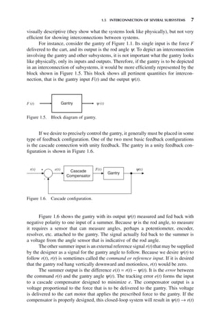
For an example of stabilization, consider the gantry shown in Figure 1.1.
Figure 1.1. Gantry.
Track
Cart (mC)
F
Rod
(mR, lR)
y
The gantry consists of a motorized cart on which is mounted a rigid rod that is free
to rotate without friction. The cart moves in one dimension along a track. A typical
gantry control objective is to move the cart from location to location along the track
with a minimum of rod sway. A practical application of this is found in industry.
Industrial gantries are used to move heavy objects from place to place in a building
or yard so that they can be worked on or serviced by different machines. It is generally
desired that the load sway as little as possible during the movement.
The gantry is open-loop stable since if the rod is displaced from the vertical-
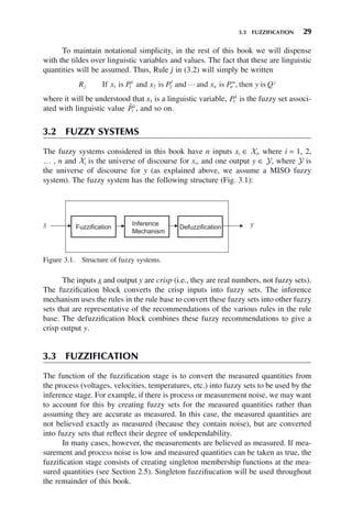
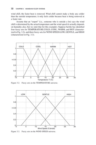
down position it will eventually return to it. However, this may take an unacceptably
long time because the gantry has very little damping. Therefore, even though the
gantry is theoretically stable as it is, we can design a controller to increase the gan-
try’s stability, that is, increase the damping so that oscillations die out more quickly.
Large industrial gantries usually use either some type of closed-loop control or an
operator with expert knowledge of how to minimize the oscillations.

23. 1.4 CONTROL 5
The inverted pendulum consists of a motorized cart on which is mounted a rigid rod
that is free to rotate without friction. The cart moves in one dimension along a track.
The inverted pendulum is open-loop unstable (i.e., in the absence of external
control), if the rod is displaced from the vertical-up position it will fall down and
never return to vertical-up. Some type of closed-loop control is necessary to maintain
the rod in the vertical-up position. The stabilization of the inverted pendulum with
a fuzzy controller is addressed in Chapter 4.
A practical application of the inverted pendulum is found in rocketry. A rocket
immediately after launch, being long and slim, tends to fall over without some type
of closed-loop control to keep it vertical. In large modern rockets, there are several
subsystems to accomplish this. One is a closed-loop control system to actuate the
base of the rocket so that it always moves underneath the rocket’s nose. This is
essentially a two- dimensional version of the inverted pendulum problem.
For an example of tracking, consider the ball and beam system of Figure 1.3.
Figure 1.2. Inverted pendulum.
Track
Cart
(mC
)
F
Rod
(mR
, lR
)
y
Figure 1.3. Ball and beam system.
Motor
Ball
Beam
y
x
For another example of stabilization, consider the inverted pendulum of
Figure 1.2.
In this system, the shaft of a direct current (DC) motor is attached to the center of
a beam along which a ball can roll. When power is supplied to the motor, the beam
rotates in the vertical plane, causing the ball to roll along it.
The ball and beam is open-loop unstable (i.e., if the ball is displaced from its
initial position, it will not return to it without some type of closed-loop control). A

24. 6 CHAPTER 1 INTRODUCTION
tracking control objective would be to actuate the motor so the ball follows a pre-
determined path at a desired velocity along the beam. The tracking problem for the
ball and beam is addressed in Chapter 10.
For a practical example of tracking, consider an annealing furnace whose
temperature must accurately follow a certain temperature profile in order to properly
anneal certain metals. This can be a difficult task for an inexperienced operator, so
closed-loop control is usually used to control the furnace temperature accurately.
For an example of model following, consider the motor-driven robotic link of
Figure 1.4.
Figure 1.4. Robotic link.
i
y
Motor
m,l
Link
This consists of a DC motor with a rigid rod attached to its shaft. The motor shaft
(hence the link) can be rotated through 360°. A true industrial robot might consist
of several of these links connected in series (with a second motor and link located
at the end of the first link, etc.).
The system is open-loop unstable, that is, if the link is displaced from its initial
angle, it will not return to it without some type of closed-loop control (unless the
initial angle was vertical-down). A model following control objective would be to
actuate the motor so the input–output behavior of the link emulates that of a refer-
ence model specified by the designer. The model following problem for the motor-
driven robotic link is addressed in Chapter 10.
For a practical example of model following, consider a small airplane being
used as a trainer for jumbo jet pilots. A model following control system can be
designed to make the small plane handle like a jumbo jet, thus obviating the need
to use large and expensive airplanes to train pilots.
1.5 INTERCONNECTION OF SEVERAL SUBSYSTEMS
The identification and control schemes in this book involve interconnections of
several subsystems. The best way to describe these is to draw a picture called a block
diagram showing blocks for each subsystem with lines labeled with the names of
the signals they contain interconnecting them. The diagrams of Figures 1.1–1.4 are

25. 1.5 INTERCONNECTION OF SEVERAL SUBSYSTEMS 7
visually descriptive (they show what the systems look like physically), but not very
efficient for showing interconnections between systems.
For instance, consider the gantry of Figure 1.1. Its single input is the force F
delivered to the cart, and its output is the rod angle ψ. To depict an interconnection
involving the gantry and other subsystems, it is not important what the gantry looks
like physically, only its inputs and outputs. Therefore, if the gantry is to be depicted
in an interconnection of subsystems, it would be more efficiently represented by the
block shown in Figure 1.5. This block shows all pertinent quantities for intercon-
nection, that is the gantry input F(t) and the output ψ(t).
Figure 1.5. Block diagram of gantry.
F (t) Gantry y (t)
Figure 1.6. Cascade configuration.
r(t) e(t) F(t) y(t)
Cascade
Compensator
Gantry
If we desire to precisely control the gantry, it generally must be placed in some
type of feedback configuration. One of the two most basic feedback configurations
is the cascade connection with unity feedback. The gantry in a unity feedback con-
figuration is shown in Figure 1.6.
Figure 1.6 shows the gantry with its output ψ(t) measured and fed back with
negative polarity to one input of a summer. Because ψ is the rod angle, to measure
it requires a sensor that can measure angles, perhaps a potentiometer, encoder,
resolver, etc. attached to the gantry. The signal actually fed back to the summer is
a voltage from the angle sensor that is indicative of the rod angle.
The other summer input is an external reference signal r(t) that may be supplied
by the designer as a signal for the gantry angle to follow. Because we desire ψ(t) to
follow r(t), r(t) is sometimes called the command or reference input. If it is desired
that the gantry rod hang vertically downward and motionless, r(t) would be zero.
The summer output is the difference e(t) = r(t) − ψ(t). It is the error between
the command r(t) and the gantry angle ψ(t). The tracking error e(t) forms the input
to a cascade compensator designed to minimize e. The compensator output is a
voltage proportional to the force that is to be delivered to the gantry. This voltage
is delivered to the cart motor that applies the prescribed force to the gantry. If the
compensator is properly designed, this closed-loop system will result in ψ(t) → r(t)

26. 8 CHAPTER 1 INTRODUCTION
as t → ∞ (i.e., asymptotic tracking). Since in this book the controllers are fuzzy, the
cascade compensator block in Figure 1.6 will be a fuzzy system.
1.6 IDENTIFICATION AND ADAPTIVE CONTROL
In the context of control, identification refers to the determination of a plant model
that is sufficient to enable the design of a controller for the plant. Identification of
linear time invariant systems is straightforwardly done using conventional methods
[4], hence fuzzy identification techniques are not necessary for such systems. Fuzzy
techniques are useful for the identification of nonlinear systems. Identification of
nonlinear systems is much less well defined than the linear case, especially if the
form of the nonlinearity is not known. Since fuzzy control is not model based, it is
not necessary to assume any particular form of the nonlinearity.
The identifier takes measurements of the plant input and output, and from these
determines a model for the plant. The fact that the plant is nonlinear is not a problem
if the identifier is fuzzy because fuzzy systems are in general nonlinear. A block
diagram depicting fuzzy identification of the gantry is shown in Figure 1.7.
Figure 1.7. Gantry identification.
In Figure 1.7, the force delivered to the gantry (or perhaps compensator output
voltage) is measured, as is the gantry rod angle. These two signals, which are volt-
ages, are fed to the identifier, which operates on them to obtain a mathematical model
of the gantry. Identification is addressed in Chapter 9.
The latter chapters of this book are concerned with adaptive fuzzy control.
Adaptive control is a method by which the system behavior is monitored online in
real time and the control continually updated and adjusted to adapt to uncertainties or
changes in the plant. There are two basic types of adaptive control: indirect and direct.
In indirect adaptive control, the plant is continually identified online, and at each time
step during the process, the controller is adjusted based on this identification. This
situation is depicted in Figure 1.8. In Figure 1.8, the arrow from the identifier going
through the compensator indicates that the compensator is being adjusted in real time
by the current mathematical model of the gantry determined by the identifier. In direct
adaptive control, which is not depicted here, the parameters of the controller are

27. 17 SUMMARY 9
directly adjusted rather than going through the intermediate step of identification.
Direct and indirect adaptive control are addressed in Chapter 10.
Figure 1.8. Indirect adaptive control of gantry.
e(t)
r(t)
F(t)
(t)
Note that block diagrams are not used in the remainder of this book. They are
only mentioned here to give the reader some idea of how the various systems in the
examples are interconnected for identification and control.
1.7 SUMMARY
Fuzzy logic is an attempt to mimic the human reasoning process. Fuzzy logic can
be used to identify and control complicated systems that would be difficult or impos-
sible to control by any other means. Expert knowledge is knowledge possessed by
human experts about a situation or problem. Expert knowledge, although invaluable
in solving complicated problems, cannot be utilized by conventional model-based
controllers. However, it is one of the great strengths of fuzzy control that expert
knowledge can be easily incorporated into fuzzy controllers.
Fuzzy identification and control is computer-intensive. Therefore, fuzzy
methods should be used only when simpler and cheaper methods, such as PID
control, cannot accomplish the control task. Fuzzy methods should generally not be
used to identify or control linear time invariant systems, as there are many well-
established methods for doing this.
The three control objectives addressed in this book are stabilization, tracking,
and model following. A system is stable if its response to bounded inputs is
bounded, or if it returns to an equilibrium state if displaced from it. The stabilization
control objective could involve stabilizing an unstable system, or increasing the
stability of an insufficiently stable system. The tracking control objective entails
forcing a system’s output to track a given reference signal. The model following
control objective entails forcing a system to emulate a reference model specified by
the designer. The stabilization, tracking, and model following control objectives will
be accomplished in this book with fuzzy identifiers and controllers.
Block diagrams are introduced in this chapter only to provide a concise
illustration of the way the fuzzy identifiers and controllers in this book will be

28. 10 CHAPTER 1 INTRODUCTION
interconnected with various example systems. The rest of this book does not contain
block diagrams.
EXERCISES
1.1 Give an example of a set of several rules you use to make some decision, for
instance, whether to go out or stay in on Saturday night. Your “rule base”
should include several rules, not just one.
1.2 Give an example of a set of several rules you use to accomplish some task,
for instance deciding how much money to invest in the stock market. Your
“rule base” should include several rules, not just one.
1.3 Give five examples of expert knowledge that you possess.
1.4 Give five examples of expert knowledge possessed by someone else of whom
you are aware.
1.5 Give two examples of systems controlled by fuzzy logic controllers other than
the examples given above. State why fuzzy control is appropriate for their
control, and why conventional nonfuzzy control would be inadequate.
1.6 Give two examples of systems controlled by conventional nonfuzzy control-
lers, and state why fuzzy control would be inappropriate for their control.
1.7 Draw block diagrams of the inverted pendulum, the motor driven robotic link,
and the ball and beam.
1.8 Draw a block diagram of the inverted pendulum in a unity feedback configu-
ration with cascade compensator.
1.9 Draw a block diagram of the motor driven robotic link with an attached
identifier.
1.10 Draw a block diagram of the ball and beam in a unity feedback configuration
with an adjustable cascade compensator being adjusted by an identifier.

29. 11
Fuzzy Control and Identification, By John H. Lilly
Copyright © 2010 John Wiley & Sons, Inc.
This book shows how fuzzy logic can be used for identification and control of
dynamic systems. The foundation of fuzzy logic is the fuzzy set. The concept of the
fuzzy set was first introduced by Zadeh in [5,6]. The fuzzy set is a generalization of
the conventional, or crisp, set that is well known to math and engineering students
(see, however, even a generalization of the fuzzy set, given in [7]). In this chapter,
we give some basic concepts of fuzzy sets that will be useful for the topics covered
in this book (i.e., fuzzy sets, universes of discourse, linguistic variables, linguistic
values, membership functions, and some associated set-theoretic operations involv-
ing them).
2.1 FUZZY SETS
For the purposes of this book, a fuzzy set is a collection of real numbers having
partial membership in the set. This is in contrast with conventional, or crisp sets, to
which a number can belong or not belong, but not partially belong. For example,
consider the set of “all heights of people 6-ft tall or taller.” This is a collection of
all real numbers ≥6. It is a crisp set because a number either belongs to this set or
does not belong to it. It is impossible for a number to partially belong to the set.
Now consider a different kind of set, the set of “heights of tall people.” A height of
7-ft tall is definitely considered tall, a height of 5-ft tall is definitely not considered
tall, and a height of 6-ft tall may be considered “kind of tall,” or tall to a certain
extent. Because numbers between five and seven can belong to the set with various
certainties, the set of “heights of tall people” is a fuzzy set.
As seen above, it takes two things to specify a fuzzy set: the members of the
set and each member’s degree of membership in the set. Total membership in
the set is specified by a membership value of 1, absolute exclusion from the set is
specified by a membership value of 0, and partial membership in the set is
specified by a membership value between 0 and 1.
If the physical quantity under consideration is described by a word (in the
above case, “height”) rather than a symbol (say, h), that word is called a linguistic
BASIC CONCEPTS OF
FUZZY SETS
CHAPTER 2

30. 12 CHAPTER 2 BASIC CONCEPTS OF FUZZY SETS
variable. Fuzzy sets are also usually given linguistic names, called linguistic values.
For instance, for the “height” variable, we could define a fuzzy set with linguistic
value “tall.” We could also define fuzzy sets with linguistic values “short” and
“medium.” Linguistic names are used for variables and their values in fuzzy logic
because people usually think and speak in linguistic terms, not mathematical
symbols.
The collection of numbers on which a variable is defined is called the universe
of discourse for the variable. For our purposes, this will usually be the field of real
numbers (ℜ). Often, though, there is an effective universe of discourse, which is a
finite sized strip of the real line (i.e., [α, β], where α < β and both are finite). For
instance, if we are considering the linguistic variable height, the universe of dis-
course would be the interval (0, ∞) because all heights would fall in this range.
However, if we are considering the heights of people, realistically the heights of
people range between about 1 and 3m. Therefore, the effective universe of discourse
for “height” would be the interval [1, 3] m.
More formally, consider a variable with universe of discourse X ⊆ ℜ, and
let x be a real number (i.e., x ∈ X). Let M denote a fuzzy set defined on X. A
membership function μM
(x) associated with M is a function that maps X into [0, 1]
and gives the degree of membership of X is M. We say that the fuzzy set M is
characterized by μM
. Then the fuzzy set M is defined as
M x x x
M
= ( )
( ) ∈
{ }
, :
μ X
This is a pairing of elements from X with their associated membership values.
For instance, the fuzzy set WARM (a linguistic value), when referring to
OUTDOOR TEMPERATURE (a linguistic variable), may be characterized by the
membership function of Figure 2.1.
Figure 2.1. Triangular membership function.
−5 0 5 10 15 20 25 30 35 40
0
0.2
0.4
0.6
0.8
1
Temperature T (°C)
Membership
µ
WARM
WARM

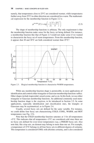
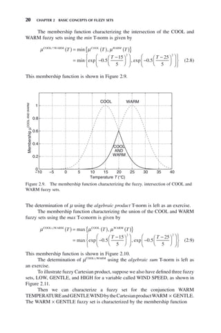
31. 2.1 FUZZY SETS 13
This is called a triangular membership function, for obvious reasons. It is defined
by the conditional function
μWARM
otherwise
T
T T
T T
( ) =
− ≤ <
− + ≤ <
⎧
⎨
⎪
⎩
⎪
0 1 1 5 15 25
0 1 3 5 25 35
0
. . ,
. . ,
,
(2.1)
where μWARM
(T) is membership in the WARM fuzzy set and T is temperature.
Note that μWARM
(T) is defined for all temperatures T even though it is zero for
some T. The universe of discourse for TEMPERATURE is the entire set of possible
temperatures (−273, ∞)°C, although there may be an effective universe of discourse
of, say, [−20, 50]°C if it is known that the temperature will never be out of this range.
The membership function indicates that a temperature of 25°C (77°F) is defi-
nitely considered warm, temperatures >25°C are decreasingly considered warm as
they increase from 25 to 35°C (95°F), and temperatures <25°C are decreasingly
considered warm as they decrease from 25 to 15°C (59°F). According to the mem-
bership function, temperatures <15°C are not considered warm at all, and tempera-
tures >35°C are also not considered warm at all. A temperature of 20°C is considered
warm to a degree 0.5 because μWARM
(20) = 0.5, and a temperature of 32°C is con-
sidered warm to a degree 0.3 because μWARM
(32) = 0.3.
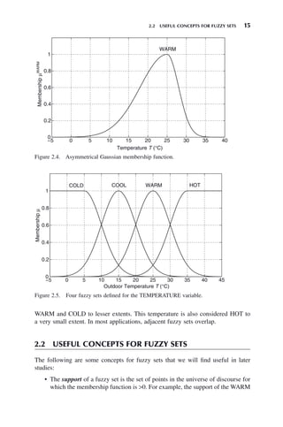
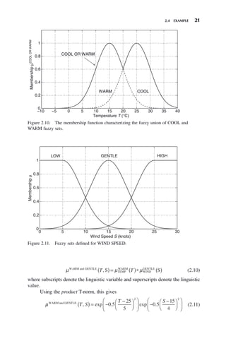
Another possibility for a membership function to characterize the WARM
fuzzy set is the Gaussian membership function of Figure 2.2. The mathematical
expression for a Gaussian function is
μ
σ
x
x c
( ) = −
−
⎛
⎝
⎜
⎞
⎠
⎟
⎛
⎝
⎜
⎞
⎠
⎟
exp
1
2
2
(2.2)
where c is the center of the function (i.e., the point at which the function attains its
maximum of 1, and σ > 0 determines the spread, or width of the function).
The membership function characterizing the WARM fuzzy set shown in
Figure 2.2 conveys similar information to the membership function of Figure 2.1,
Figure 2.2. Gaussian membership function.
−5 0 5 10 15 20 25 30 35 40
0.2
0.4
0.6
0.8
1
Temperature T (°C)
Membership
μ
WARM
WARM

32. 14 CHAPTER 2 BASIC CONCEPTS OF FUZZY SETS
namely, that temperatures close to 25°C are considered warmer, while temperatures
further away from 25°C in either direction are considered less warm. The mathemati-
cal expression for the membership function in Figure 2.2 is
μWARM
T
T
( ) = −
−
⎛
⎝
⎜
⎞
⎠
⎟
⎛
⎝
⎜
⎞
⎠
⎟
exp
1
2
25
5
2
(2.3)
The shape of membership functions is arbitrary. The only requirement is that
the membership function make sense for the fuzzy set being defined. For instance,
a membership function like that of Figure 2.3 would not make sense if we wanted
to characterize the fuzzy set of warm temperatures. From this membership function,
it appears that 20 and 30°C are both considered warmer than 25°C!
Figure 2.3. Illogical membership function to characterize WARM temperatures.
−5 0 5 10 15 20 25 30 35 40
0
0.2
0.4
0.6
0.8
1
Temperature T (°C)
Membership
μ
WARM
WARM?
While any membership function shape is permissible, in most applications of
identification and control either triangular or Gaussian membership functions suffice.
Other shapes include trapezoidal, raised cosine, and so on. In this book, we use either
triangular or Gaussian membership functions. An additional commonly used mem-
bership function shape is the singleton, to be introduced in Section 2.5. In some
applications, especially identification and classification ones, the triangles or
Gaussians may be asymmetrical, as in Figure 2.4.
Usually, several fuzzy sets are defined for the same variable. For instance,
we could define four fuzzy sets characterizing COLD, COOL, WARM, and HOT
temperatures (see Fig. 2.5).
Note that the COLD membership function saturates at 1 for all temperatures
<5°C. This indicates that all temperatures <5°C are considered cold since there are
no fuzzy sets defined for even lower temperatures (say, a FRIGID fuzzy set). Also
note that, like crisp sets, an element may belong to more than one set. For example,
a temperature of 15°C belongs to all four fuzzy sets to different degrees of certainty.
This temperature is considered COOL with absolute certainty, and is also considered

33. 2.2 USEFUL CONCEPTS FOR FUZZY SETS 15
WARM and COLD to lesser extents. This temperature is also considered HOT to
a very small extent. In most applications, adjacent fuzzy sets overlap.
2.2 USEFUL CONCEPTS FOR FUZZY SETS
The following are some concepts for fuzzy sets that we will find useful in later
studies:
• The support of a fuzzy set is the set of points in the universe of discourse for
which the membership function is >0. For example, the support of the WARM
Figure 2.4. Asymmetrical Gaussian membership function.
−5 0 5 10 15 20 25 30 35 40
0
0.2
0.4
0.6
0.8
1
Temperature T (°C)
Membership
μ
WARM
WARM
Figure 2.5. Four fuzzy sets defined for the TEMPERATURE variable.
−5 0 5 10 15 20 25 30 35 40 45
0
0.2
0.4
0.6
0.8
1
Outdoor Temperature T (°C)
Membership
μ
COLD COOL WARM HOT

34. 16 CHAPTER 2 BASIC CONCEPTS OF FUZZY SETS
fuzzy set in Figure 2.1 is the open interval (15, 35)°C. The support of the
WARM fuzzy set in Figure 2.2 is (−273, ∞)°C.
• An α-cut of a fuzzy set is the set of points in the universe of discourse where
the membership function is >α. It is the collection of all members of the set
with a certain minimum degree of membership. For example, the 0.5-cut of
the fuzzy set in Figure 2.1 is (20, 30)°C. The 0.5-cut of the fuzzy set in Figure
2.2 is (19.1129, 30.8871)°C.
• The height of a fuzzy set is the peak value reached by its membership func-
tion. This is usually 1.
• A normal fuzzy set is a fuzzy set whose membership function reaches 1 for
at least one point in the universe of discourse.
• A convex fuzzy set is a fuzzy set whose membership function satisfies
μ λ λ μ μ
x x x x
1 2 1 2
1
+ −
( )
( ) ≥ ( ) ( )
( )
min , (2.4)
∀(x1, x2) and ∀λ ∈ (0, 1]. The concept of a convex fuzzy set is not to be confused
with the concept of a convex function, although the definitions look similar. Many
membership functions are not convex as functions, although they characterize
convex fuzzy sets. The fuzzy sets of Figures 2.1 and 2.2 are convex, although the
membership function of Figure 2.2 is not a convex function. The fuzzy set of Figure
2.3 is not convex. Nonconvex fuzzy sets are legal in fuzzy systems, as long as they
accurately represent their corresponding quantity.
2.3 SOME SET-THEORETIC AND LOGICAL
OPERATIONS ON FUZZY SETS
It is possible to define concepts (subset, compliment, intersection, union, etc.) for
fuzzy sets similarly to crisp sets. Below we give some of the more often-used opera-
tions on fuzzy sets.
Fuzzy Subset
Let M1
and M2
be two fuzzy sets defined for a variable on the universe of
discourse X, and let their associated membership functions be μ1
(x) and
μ2
(x), respectively. Then, M1
is a fuzzy subset of M2
(or M1
⊆ M2
) if
μ1
(x) ≤ μ2
(x)∀x ∈ X.
Fuzzy Compliment
Consider a fuzzy set M defined for a variable on the universe of discourse X,
and let M have associated membership function μM
(x). The fuzzy compli-
ment of M is a fuzzy set M̄ characterized by membership function
μM̄
(x) = 1 − μM
(x).
Fuzzy Intersection (AND)
Let M1
and M2
be two fuzzy sets defined for a variable on the universe
of discourse X, and let their associated membership functions be

35. 2.3 SOME SET-THEORETIC AND LOGICAL OPERATIONS ON FUZZY SETS 17
μ1
(x) and μ2
(x), respectively. The fuzzy intersection of M1
and M2
,
denoted by M1
傽 M2
, is a fuzzy set with membership function
(1) μ μ μ
M M
x x x x
1 2 2
艚
( ) = ( ) ( ) ∈
{ }
1
min , : X (minimum) or (2)
μ μ μ
M M
x x x x
1 2 2
艚
( ) = ( ) ( ) ∈
{ }
1
: X (algebraic product).
Notice that we give two possibilities to characterize the intersection of two
fuzzy sets: min and algebraic product. There are other methods that can be
used to represent intersection as well [8–13]. In general, we could use any
operation on the two membership functions μ1
(x) and μ2
(x) that satisfies
the common-sense requirements:
1. An element in the universe cannot belong to the intersection of two
fuzzy sets to a greater degree than it belongs to either one of the fuzzy
sets individually.
2. If an element does not belong to one of the fuzzy sets, then it cannot
belong to the intersection of that fuzzy set and another fuzzy set.
3. If an element belongs to both fuzzy sets with absolute certainty, then it
belongs to the intersection of the two fuzzy sets with absolute
certainty.
Since the membership function values are between 0 and 1, the operations of
minimum and product both satisfy the above three requirements. These two
operations are found to suffice for most fuzzy systems.
If we use the notation * to represent the AND operation, then the membership
function characterizing the fuzzy intersection of M1
and M2
can be generi-
cally written as μ μ μ
M M
x x x
1 2 2
艚
( ) = ( )∗ ( )
1
. The * operation (whether min,
product, or other) is called a triangular norm or T-norm.
Fuzzy Union (Or)
Let M1
and M2
be two fuzzy sets defined for a variable on the universe
of discourse X, and let their associated membership functions be
μ1
(x) and μ2
(x), respectively. The fuzzy union of M1
and M2
, denoted by
M1
傼 M2
, is a fuzzy set with membership function (1) μM M
x
1 2
艛
( ) =
max , :
μ μ
1
( ) ( ) ∈
{ }
x x x
2
X (maximum) or (2) μM M
x
1 2
艛
( ) =
μ μ μ μ
1 1
( )+ ( )− ( ) ( ) ∈
{ }
x x x x x
2 2
: X (algebraic sum).
Notice that we give two possibilities to characterize the union of two fuzzy
sets: max and algebraic sum. There are other methods that can be used to
represent union as well (see the above references). In general, we could use
any operation on the two membership functions μ1
(x) and μ2
(x) that satisfies
the common-sense requirements:
1′. An element in the universe cannot belong to the union of two fuzzy sets
to a lesser degree than it belongs to either one of the fuzzy sets
individually.
2′. If an element belongs to one of the fuzzy sets, then it must belong to
the union of that fuzzy set and another fuzzy set.

36. 18 CHAPTER 2 BASIC CONCEPTS OF FUZZY SETS
3′. If an element does not belong to either fuzzy set, then it cannot belong
to the union of the two fuzzy sets.
Since the membership function values are between 0 and 1, the operations of
maximum and algebraic sum both satisfy requirements 1′–3′. These two
operations are found to suffice for most fuzzy systems.
If we use the notation ⊕ to represent the OR operation, then the membership
function characterizing the fuzzy union of M1
and M2
can be written as
μ μ μ
M M
x x x
1 2 2
艛
( ) = ( )⊕ ( )
1
. The ⊕ operation (whether max, algebraic
sum, or other) is called a triangular conorm or T-conorm.
Fuzzy Cartesian Product
Cartesian product refers to combining fuzzy sets defined for different variables
on different universes of discourse. If M j
1 , Mk
2, … , Mn
l
are fuzzy sets
defined on the universes X1, X2, … , Xn, respectively, with fuzzy set Mi
m
characterized by membership function μi
m
, their Cartesian product is a
fuzzy set, denoted by M M M
j k
n
l
1 2
× × ×
, characterized by the member-
ship function
μ μ μ μ
M M M
n
j k l
n
j K
n
x x x x x x
1 2
1
1 2 1 1 2 2 1
× × ×
( ) = ( )∗ ( )∗ ∗ ( )
…
, , , (2.5)
where the T-norm * is defined as above (min, product, etc.).
2.4 EXAMPLE
Let the COMFORTABLE ROOM TEMPERATURE (CRT) fuzzy set be character-
ized by the membership function
μCRT
T
T
( ) = −
−
⎛
⎝
⎜
⎞
⎠
⎟
⎛
⎝
⎜
⎞
⎠
⎟
exp .
0 5
25
2
2
(2.6)
which is shown in Figure 2.6.
Figure 2.6. Membership function for CRT fuzzy set.
−5 0 5 10 15 20 25 30 35 40
0
0.2
0.4
0.6
0.8
1
Temperature T (°C)
Membership
μ
CRT
CRT

37. 2.4 EXAMPLE 19
Now it is clear that the CRT fuzzy set is a subset of the WARM fuzzy set
shown in Figure 2.2, because μCRT
(T) ≤ μWARM
(T)∀T. A plot of μCRT
(T) and μWARM
(T)
together is shown in Figure 2.7.
Figure 2.7. Graphical illustration of a fuzzy subset.
−5 0 5 10 15 20 25 30 35 40
0
0.2
0.4
0.6
0.8
1
Temperature T (°C)
Membership
μ
WARM
CRT
The compliment of the WARM fuzzy set (i.e., the NOT WARM) or WARM
fuzzy set, is characterized by the membership function
μWARM
T
T
( ) = − −
−
⎛
⎝
⎜
⎞
⎠
⎟
⎛
⎝
⎜
⎞
⎠
⎟
1 0 5
25
5
2
exp . (2.7)
and shown in Figure 2.8.
−10 −5 0 5 10 15 20 25 30 35 40
0
0.2
0.4
0.6
0.8
1
Temperature T (°C)
Membership
μ
NOT
WARM
NOT WARM
Figure 2.8. Membership function characterizing the NOT WARM fuzzy set.

38. 20 CHAPTER 2 BASIC CONCEPTS OF FUZZY SETS
Figure 2.9. The membership function characterizing the fuzzy. intersection of COOL and
WARM fuzzy sets.
−10 −5 0 5 10 15 20 25 30 35 40
0
0.2
0.4
0.6
0.8
1
Temperature T (°C)
Membership
μ
COOL
AND
WARM
COOL WARM
COOL
AND
WARM
The membership function characterizing the intersection of the COOL and
WARM fuzzy sets using the min T-norm is given by
μ μ μ
COOL WARM
艚
T T T
T
COOL WARM
( ) = ( ) ( )
{ }
= −
−
⎛
⎝
⎜
⎞
⎠
⎟
min ,
min exp .
0 5
15
5
2 2
0 5
25
5
⎛
⎝
⎜
⎞
⎠
⎟ −
−
⎛
⎝
⎜
⎞
⎠
⎟
⎛
⎝
⎜
⎞
⎠
⎟
⎧
⎨
⎩
⎫
⎬
⎭
, exp .
T
(2.8)
This membership function is shown in Figure 2.9.
The determination of μ using the algebraic product T-norm is left as an exercise.
The membership function characterizing the union of the COOL and WARM
fuzzy sets using the max T-conorm is given by
μ μ μ
COOL WARM COOL WARM
艛
T T T
T
( ) = ( ) ( )
{ }
= −
−
⎛
⎝
⎜
⎞
⎠
⎟
max ,
max exp .
0 5
15
5
2 2
0 5
25
5
⎛
⎝
⎜
⎞
⎠
⎟ −
−
⎛
⎝
⎜
⎞
⎠
⎟
⎛
⎝
⎜
⎞
⎠
⎟
⎧
⎨
⎩
⎫
⎬
⎭
, exp .
T
(2.9)
This membership function is shown in Figure 2.10.
The determination of μCOOL傼WARM
using the algebraic sum T-norm is left as
an exercise.
To illustrate fuzzy Cartesian product, suppose we also have defined three fuzzy
sets, LOW, GENTLE, and HIGH for a variable called WIND SPEED, as shown in
Figure 2.11.
Then we can characterize a fuzzy set for the conjunction WARM
TEMPERATUREandGENTLEWINDbytheCartesianproductWARM × GENTLE.
The WARM × GENTLE fuzzy set is characterized by the membership function

39. 2.4 EXAMPLE 21
μ μ μ
WARM and GENTLE
TEMP
WARM
WIND
GENTLE
S S
T T
,
( ) = ( )∗ ( ) (2.10)
where subscripts denote the linguistic variable and superscripts denote the linguistic
value.
Using the product T-norm, this gives
μWARM and GENTLE
T S
T S
, exp . exp .
( ) = −
−
⎛
⎝
⎜
⎞
⎠
⎟
⎛
⎝
⎜
⎞
⎠
⎟ −
−
⎛
0 5
25
5
0 5
15
4
2
⎝
⎝
⎜
⎞
⎠
⎟
⎛
⎝
⎜
⎞
⎠
⎟
2
(2.11)
Figure 2.10. The membership function characterizing the fuzzy union of COOL and
WARM fuzzy sets.
−10 −5 0 5 10 15 20 25 30 35 40
0
0.2
0.4
0.6
0.8
1
Temperature T (°C)
Membership
μ
COOL
OR
WARM
COOL OR WARM
COOL
WARM
Figure 2.11. Fuzzy sets defined for WIND SPEED.
0 5 10 15 20 25 30
0
0.2
0.4
0.6
0.8
1
Wind Speed S (knots)
Membership
μ
GENTLE HIGH
LOW

40. 22 CHAPTER 2 BASIC CONCEPTS OF FUZZY SETS
Note that μWARMandGENTLE
(T, S) is a function of two variables (temperature T and
wind speed S ), so when plotted it will be a three-dimensional surface over the T–S
plane (see Fig. 2.12).
Figure 2.12. Membership function for WARM GENTLE fuzzy set.
−10
0
10
20
30
0
10
20
30
40
50
0
0.2
0.4
0.6
0.8
1
Wind Speed S (knots)
Temperature T (°C)
μ
WARMGENTLE
According to the membership function of Figure 2.12, a temperature of 25°C
together with a wind speed of 15 knots is classified as WARMGENTLE with
certainty 1 (i.e., absolute certainty), a temperature of 20°C together with a wind
speed of 20 knots is classified as WARMGENTLE with certainty 0.2777, and a
temperature of 28°C together with a wind speed of 13 knots is classified as
WARMGENTLE with certainty 0.7371.
2.5 SINGLETON FUZZY SETS
Another type of fuzzy set that is used extensively in fuzzy systems (see Chapter 3)
is the singleton fuzzy set. This type of set contains only one member, and that
member’s degree of belongingness to the set is unity. Suppose we create five single-
ton fuzzy sets on the VOLTAGE universe of discourse such that a NEGATIVE
LARGE (NL) voltage is defined as exactly −1V, a NEGATIVE SMALL (NS)
voltage is defined as exactly −0.5V, a ZERO (Z) voltage is defined as exactly 0V,
a POSITIVE SMALL (PS) voltage is defined as exactly 0.5V, and a POSITIVE
LARGE (PL) voltage is defined as exactly 1V. We can consider these five voltages
as the only members of five singleton fuzzy sets characterized by the membership
functions shown in Figure 2.13.
Although it seems unnecessarily complicated to do this, the characterization
of certain quantities as members of singleton fuzzy sets is very useful for fuzzifica-
tion and certain output fuzzy sets (see Chapter 3).

41. 2.6 SUMMARY 23
2.6 SUMMARY
Real-world processes, whether they are electrical systems, mechanical systems, heat
transfer systems, financial systems, or whatever, involve crisp quantities. When you
invest, you must invest an exact quantity of money, say $1000, not “a lot of money.”
When you make a pizza, you must set the oven to an exact temperature, say 450°F,
you do not turn it up until it’s “pretty hot.”
The fuzzy reasoning process cannot deal with crisp numbers like these. It is
modeled after the human reasoning process, which is also not very efficient at
dealing with crisp numbers. When we make decisions, we usually make them based
on our feelings, perceptions, past experience, and intuition. Our brains are very
efficient at deciding things this way. When deciding how much of a tip to leave the
waiter, we might say to ourselves, “the service was prompt, so I will leave a nice
tip” and be done with it, instead of, “my food was brought in 10.25min, so my tip
will be 15% plus 2.5% times the number of minutes less than the average response
time it took to bring my food.”
Fuzzy identification and control use fuzzy reasoning processes to make
decisions about how to model and/or control real-world systems. Since real-
world systems operate in the crisp realm and fuzzy reasoning cannot deal with crisp
quantities, fuzzy sets are used as a means of translating between the two. As will
be seen, the translation goes both ways. Fuzzy sets are used to convert crisp
numbers from the real world into fuzzy quantities that can be utilized by the fuzzy
reasoning process. Fuzzy sets are also used to convert the recommendations of the
fuzzy reasoning process into crisp numbers that can be utilized by the real-world
process.
Figure 2.13. Membership functions characterizing five singleton fuzzy sets.
−1.5 −1 −0.5 0 0.5 1 1.5
0
0.2
0.4
0.6
0.8
1
Voltage (V)
Membership
μ
NL NS Z PS PL

42. 24 CHAPTER 2 BASIC CONCEPTS OF FUZZY SETS
The main topics of this chapter include the following:
1. Fuzzy Set. A crisp pairing consisting of members of the set and their degree
of membership in the set. In this book, we consider quantities to be members
of only triangular, Gaussian, or singleton fuzzy sets.
2. Linguistic Variable. A linguistic name that people use to name a quantity, as
opposed to a mathematical symbol (“temperature” rather than t).
3. Linguistic Value. A linguistic name that people use to quantify something
(“very fast” rather than 75mph).
4. Universe of Discourse. The set of all possible values for a linguistic
variable.
5. Membership Function. A function that maps a universe of discourse into [0,
1] and that describes the degree of membership of every member of the uni-
verse in a particular fuzzy set.
6. Support of a Fuzzy Set. The set of points for which the membership function
is 0.
7. α-Cut of a Fuzzy Set. The set of points for which the membership function
is α.
8. Height of Fuzzy Set. The peak value reached by its membership function.
9. Normal Fuzzy Set. A fuzzy set whose membership function reaches a value
of 1 for at least one point in the universe.
10. Convex Fuzzy Set. A fuzzy set whose membership function μ satisfies
μ(λx1 + (1 − λ)x2) ≥ min(μ(x1), μ(x2)) ∀ (x1, x2) and ∀λ ∈ (0, 1].
11. T-Norm (Triangular Norm). Any operation between fuzzy sets that preserves
the three axioms 1–3 in Section 2.3.
12. T-Conorm (Triangular Conorm). Any operation between fuzzy sets that
preserves the three axioms 1′–3′ in Section 2.3.
13. Fuzzy Subset. A fuzzy set all of whose members also belong to another fuzzy
set on the same universe.
14. Fuzzy Compliment. A fuzzy set whose members also belong to another fuzzy
set on the same universe with inverse belongingness.
15. Fuzzy Intersection. A fuzzy set whose members also belong to several other
fuzzy sets that are all on the same universe.
16. Fuzzy Union. A fuzzy set whose members also belong to any of several other
fuzzy sets that are all on the same universe
17. Fuzzy Cartesian Product. A fuzzy set whose members also belong to several
other fuzzy sets that are all on different universes.
EXERCISES
2.1 Give mathematical expressions for μ1(x) and μ2(x) shown below (Figs. 2.14
and 2.5).

43. EXERCISES 25
Figure 2.14. Gaussian membership function for Problem 2.1.
0 10 20 30 40 50 60 70 80
0
0.2
0.4
0.6
0.8
1
x
μ
1
(x)
Figure 2.15. Triangular membership function for Problem 2.1.
−20 −15 −10 −5 0 5 10 15 20 25 30
0
0.2
0.4
0.6
0.8
1
x
μ
2
(x)
2.2 Calculate the mathematical expressions for the Gaussian memberships in
Figures 2.5 and 2.11.
2.3 (a) Specify a fuzzy set for all “fast” car speeds. (b) Specify five fuzzy sets
on the “car speed” universe of discourse.
2.4 Plot the membership function characterizing the COOL 傽 WARM fuzzy set
in the example in Section 2.4 using algebraic product for the T-norm.
2.5 Plot the membership function characterizing the COOL 傼 WARM fuzzy set
in the example in Section 2.4 using algebraic sum for the T-norm.

44. 26 CHAPTER 2 BASIC CONCEPTS OF FUZZY SETS
2.6 Plot the membership function characterizing the fuzzy set that is the Cartesian
product of WARM temperatures and GENTLE winds in the example in
Section 2.4 using minimum for the T-norm.
2.7 What is the 0.1-cut of the COOL fuzzy set in Figure 2.5?
2.8 Is the fuzzy set characterized by the trapezoidal membership function shown
in Fig. 2.16 convex? What is its support? What is its 0.1-cut?
Figure 2.16. Trapezoidal membership function for Problem 2.8.
µ(x)
1
–20 –8 0 8 20 x
2.9 Is the WARM fuzzy set characterized by the Gaussian membership function
of Figure 2.2 a fuzzy subset of the WARM fuzzy set characterized by the
triangular membership function of Figure 2.1? Answer the same question
with the sets reversed (i.e., is the set of Fig. 2.1 a subset of that of Fig. 2.2?).
2.10 Plot the membership function characterizing the fuzzy set that is the union
of the WARM fuzzy set whose membership is shown in Figure 2.1 and the
COOL fuzzy set whose membership is shown in Figure 2.5. Use both
T-conorms discussed above.

45. 27
Fuzzy Control and Identification, By John H. Lilly
Copyright © 2010 John Wiley Sons, Inc.
A system is a combination of components that as a whole operate on a vector of
input functions of time x(t) ∈ ℜn
for each t to produce a vector of output functions
of time y(t) ∈ ℜm
for each t. A fuzzy system is a system that uses fuzzy logic to
operate on the input x(t) to produce the crisp output y(t). It can be shown that a fuzzy
system with n inputs and m outputs (i.e., a multi-input multi-output, or MIMO fuzzy
system) is equivalent to m fuzzy systems, each with n inputs and one output (i.e.,
multi-input single-output, or MISO fuzzy systems). Therefore, we will study only
MISO fuzzy systems in this book. All fuzzy controllers and identifiers are fuzzy
systems.
3.1 IF-THEN RULES AND RULE BASE
Much of human decision making occurs in the form of “if-then” rules. The four
forms of if-then rules in classical logic are called modus ponendo ponens (Latin for
“mode that affirms by affirming”) or simply modus ponens, modus tollendo tollens
(Latin for “mode that denies by denying”), or simply modus tollens, modus ponendo
tollens (Latin for “mode that denies by affirming”), and modus tollendo ponens
(Latin for “mode that affirms by denying”).
For examples of these, consider the problem of steering a vehicle toward a
target in the presence of an obstacle. Possible rules for deciding which way to steer
might be (this is not a complete set):
1. If the target direction is ahead, then the steering direction is straight (modus
ponendo ponens).
2. If the obstacle direction is ahead then the steering direction is not straight
(modus ponendo tollens).
3. If the obstacle direction is not ahead then the steering direction is straight
(modus tollendo ponens).
4. If the target direction is not ahead then the steering direction is not straight
(modus tollendo tollens).
MAMDANI FUZZY SYSTEMS
CHAPTER 3

46. 28 CHAPTER 3 MAMDANI FUZZY SYSTEMS
In statement 1, the recommendation to steer straight is affirmed by affirming
that the target is ahead. In statement 2, the recommendation to steer straight is denied
by affirming that an obstacle is ahead. In statement 3, the recommendation to steer
straight is affirmed by denying that the obstacle is ahead. In statement 4, the recom-
mendation to steer straight is denied by denying that the target is ahead. Of course,
a complete set of rules for steering to a target in the presence of obstacles would
require more rules than the above. People reason in all of these ways. All of these
modes of reasoning can be implemented with fuzzy logic (see [14] and [15] for
practical examples of controllers employing modus ponendo tollens logic).
The vast majority of if-then rules used in fuzzy control and identification are
of the modus ponens form. For example, consider the rule Ri:
R x P y Q
i If is then is
, (3.1)
where x̃is a linguistic variable defined on universe X, P̃ is a linguistic value described
by fuzzy set P defined on universe X, ỹ is a linguistic variable defined on universe
Y, and Q̃ is a linguistic value described by fuzzy set Q defined on universe Y. A
tilde over a symbol indicates a linguistic variable or value.
The first part of the statement, “x̃ is P̃,” is called the premise of the rule, and
the second part of the statement, “ỹ is Q̃ ” is called the consequent of the rule. The
consequent of the rule is affirmed by affirming the premise—if the premise is true,
the consequent is also true.
An example of an if-then rule in modus ponens form pertaining to stopping a
car is, “If SPEED is FAST then BRAKE PRESSURE is HEAVY.” In this rule,
SPEED is FAST is the premise and BRAKE PRESSURE is HEAVY is the conse-
quent. SPEED is the input linguistic variable, FAST is a linguistic value of SPEED
and is a fuzzy set on the SPEED universe, BRAKE PRESSURE is the output lin-
guistic variable, and HEAVY is a linguistic value of BRAKE PRESSURE and is a
fuzzy set on the BRAKE PRESSURE universe.
Note that there may be more than one part to the premise, that is, we could
have the rule Rj:
R x P x P x P y Q
j
k l
n n
m j
If is and is and and is then is
1 1 2 2 , (3.2)
In this rule, the premise is a conjunction of n conditions: x̃1 is
Pk
1 and x̃2 is
Pl
2
and … and x̃n is
Pn
m
. For example, another rule about stopping a car might be, “If
SPEED is FAST and GRADE is DOWNHILL then BRAKE PRESSURE is VERY
HEAVY.”
In general, we use a number of rules to accomplish a task. Several rules are
needed to specify actions to be taken under different conditions. The collection of
rules as a whole is called a Rule base. A simple rule base for stopping a car
might be
1. If SPEED is SLOW, then BRAKE PRESSURE is LIGHT.
2. If SPEED is MEDIUM, then BRAKE PRESSURE is MEDIUM.
3. If SPEED is FAST, then BRAKE PRESSURE is HEAVY.

47. 3.3 FUZZIFICATION 29
To maintain notational simplicity, in the rest of this book we will dispense
with the tildes over linguistic variables and values. The fact that these are linguistic
quantities will be assumed. Thus, Rule j in (3.2) will simply be written
R x P x P x P y Q
j
k l
n n
m j
If is and is and and is then is
1 1 2 2 ,
where it will be understood that x1 is a linguistic variable, Pk
1 is the fuzzy set associ-
ated with linguistic value
Pk
1 , and so on.
3.2 FUZZY SYSTEMS
The fuzzy systems considered in this book have n inputs xi ∈ Xi, where i = 1, 2,
… , n and Xi is the universe of discourse for xi, and one output y ∈ Y, where Y is
the universe of discourse for y (as explained above, we assume a MISO fuzzy
system). The fuzzy system has the following structure (Fig. 3.1):
Figure 3.1. Structure of fuzzy systems.
The inputs x and output y are crisp (i.e., they are real numbers, not fuzzy sets).
The fuzzification block converts the crisp inputs into fuzzy sets. The inference
mechanism uses the rules in the rule base to convert these fuzzy sets into other fuzzy
sets that are representative of the recommendations of the various rules in the rule
base. The defuzzification block combines these fuzzy recommendations to give a
crisp output y.
3.3 FUZZIFICATION
The function of the fuzzification stage is to convert the measured quantities from
the process (voltages, velocities, temperatures, etc.) into fuzzy sets to be used by the
inference stage. For example, if there is process or measurement noise, we may want
to account for this by creating fuzzy sets for the measured quantities rather than
assuming they are accurate as measured. In this case, the measured quantities are
not believed exactly as measured (because they contain noise), but are converted
into fuzzy sets that reflect their degree of undependability.
In many cases, however, the measurements are believed as measured. If mea-
surement and process noise is low and measured quantities can be taken as true, the
fuzzification stage consists of creating singleton membership functions at the mea-
sured quantities (see Section 2.5). Singleton fuzzifiucation will be used throughout
the remainder of this book.

48. 30 CHAPTER 3 MAMDANI FUZZY SYSTEMS
3.4 INFERENCE
The first function of the inference stage is to determine the degree of firing of each
rule in the rule base. Consider rule Ri (3.1), which has a single input x. Let fuzzy
set P be characterized by the membership function μP
(x), and fuzzy set Q be char-
acterized by the membership function μQ
(y). For a particular crisp input x ∈ X, we
say rule Ri is fired, or is on (i.e., it is taken as true) to the extent μP
(x). As mentioned
in Chapter 2, this is a real number in the interval [0, 1]. More generally, we call
fuzzy set P the premise fuzzy set for Rule i, and μP
, which we will call μi, the premise
membership function for Rule i. Then, for a particular real input x, rule Ri is fired
(or is on) to the extent μi(x).
Now consider rule Rj (3.2), which has n inputs x1, x2, … , xn. Let the fuzzy set
P P P
k l
n
m
1 2
× × ×
be characterized by the membership function μP P P
k l
n
m
1 2
× × ×
. For a
particular real input x = (x1, x2, … , xn) ∈ X1 × X2 × … × Xn, we say rule Rj is fired
to the extent μ μ μ μ
P P P k l
n
m
n
k l
n
m
x x x x
1 2
1 1 2 2
× × ×
( ) = ( )∗ ( )∗ ∗ ( )
[see (2.5)]. This is a real
number in the interval [0, 1]. More generally, we call fuzzy set P P P
k l
n
m
1 2
× × ×
the
premise fuzzy set for Rule Rj and μP P P
k l
n
m
1 2
× × ×
, which we will call μj, the premise
membership function for Rule j. Then for a particular real input x, rule Rj is fired (or
is on) to the extent μ μ μ μ
j
k l
n
m
n
x x x x
( ) = ( )∗ ( )∗ ∗ ( )
1 1 2 2 .
The second function of the inference stage is to determine the degree to which
each rule’s recommendation is to be weighted in arriving at the final decision and
to determine an implied fuzzy set corresponding to each rule. Consider rule Rj (3.2)
with input x = (x1, x2, … , xn). From the discussion above, we know this rule is fired
to the degree μj(x). Therefore we attenuate the recommendation of rule Rj, which is
fuzzy set Qj
characterized by μQ j
y
( ), by μj(x). This produces an implied fuzzy set
Q̂j
defined on Y, characterized by the membership function
μ μ μ
Q̂
j
Q
j j
y x y
( ) = ( )∗ ( ) (3.3)
If there are R rules in the form of (3.2), each rule has its own premise member-
ship function μj(x), j = 1, 2, … , R. The R rules produce R implied fuzzy sets Q̂j
, j = 1,
2, … , R, each characterized by a membership function calculated as in (3.3). Note
that μQ j
y
( ) and μQ̂ j
y
( ) are defined ∀y ∈ Y. On the other hand, the degree of firing
of rule j, μj(x), is a function of a particular real vector x ∈ ℜn
, hence is a real number.
In summary, the function of the inference stage is twofold: (1) to determine
the degree of firing of each rule in the rule base, and (2) to create an implied fuzzy
set for each rule corresponding to the rule’s degree of firing.
3.5 DEFUZZIFICATION
The function of the defuzzification stage is to convert the collection of recommenda-
tions of all rules into a crisp output. Consider a rule base consisting of R rules of
the form (3.2). Then, we have R implied fuzzy sets, one from each rule, each recom-
mending a particular outcome. In order to arrive at one crisp output y, we combine
all of these recommendations by taking a weighted average of the various recom-
mendations. There are several ways to do this, but perhaps the two most common

49. 3.6 EXAMPLE: FUZZY SYSTEM FOR WIND CHILL 31
are center of gravity (COG) defuzzification, and center average (CA)
defuzzification.
3.5.1 Center of Gravity (COG) Defuzzification
Suppose the consequent fuzzy set of Rule i is Qi
, characterized by membership
μQi
y
( ). Define the center of area of μQi
y
( ) to be the point qi in the universe Y with
the property that
μ μ
Q
q
Q
q
i
i
i
i
y dy y dy
( ) = ( )
−∞
∞
∫ ∫ (3.4)
Then, the crisp output of the fuzzy system is calculated using COG
defuzzification as
y
qi
Q
i
R
Q
i
R
i
i
crisp
=
∫
∑
∫
∑
=
=
μ
μ
ˆ
ˆ
1
1
(3.5)
where μQ̂i
∫ is the area under μQ̂i
. The expression in (3.5) is a weighted average of
the qi’s, i = 1, … , R.
3.5.2 Center Average (CA) Defuzzification
Suppose the consequent fuzzy set of Rule i is Qi
, characterized by membership
μQi
y
( ). Then the crisp output of the fuzzy system is calculated using CA defuzzi-
fication as
y
q y
y
i
y
Q
i
R
y
Q
i
R
i
i
crisp =1
=1
max
max
=
{ }
{ }
∑
∑
μ
μ
ˆ
ˆ
( )
( )
(3.6)
Note that if Qi
is normal (it usually is), then max
y
Q
i
i
y x
μ μ
ˆ
( )
{ }= ( ) whether min or
prod is used as the T-norm in (3.3). In that case, CA defuzzification gives
y
q x
x
i i
i
R
i
i
R
crisp
=
( )
( )
=
=
∑
∑
μ
μ
1
1
(3.7)
3.6 EXAMPLE: FUZZY SYSTEM FOR WIND CHILL
Consider a fuzzy system to determine what the temperature feels like to a person
under certain weather conditions. This is known as “wind chill.” Wind chill has to
do with the rate at which heat is removed from the person’s body—the lower the

50. 32 CHAPTER 3 MAMDANI FUZZY SYSTEMS
Figure 3.2. Fuzzy sets on the TEMPERATURE universe.
−5 0 5 10 15 20 25 30 35
0
0.2
0.4
0.6
0.8
1
Temperature T (°C)
μ
COLD COOL WARM HOT
Figure 3.3. Fuzzy sets on the WIND SPEED universe.
0 5 10 15 20 25 30
0
0.2
0.4
0.6
0.8
1
Wind Speed S (knots)
μ
LOW GENTLE HIGH
wind chill, the faster heat is removed. Wind chill cannot make a body any colder
than the outside temperature; it only feels colder because heat is being removed at
a faster rate.
Assume that an “expert” (i.e., someone who is outside a lot) says the wind
chill is determined by the actual temperature and the wind speed (it actually depends
on humidity also, but we omit that for this example). Suppose he/she has identified
four fuzzy sets for TEMPERATURE:COLD, COOL, WARM, and HOT (character-
ized in Fig. 3.2), and three fuzzy sets for WIND SPEED:LOW, GENTLE, and HIGH
(characterized in Fig. 3.3).

51. 3.6 EXAMPLE: FUZZY SYSTEM FOR WIND CHILL 33
Suppose also that he/she has identified five fuzzy sets for WIND CHILL:SEVERE,
BAD, BEARABLE, MILD, and UNNOTICEABLE, characterized on the output
universe of discourse as in Figure 3.4.
Notice from Figure 3.4 that the end memberships on the output universe (i.e.,
SEVERE and UNNOTICEABLE) do not saturate at 1 as the end memberships on
the input universes do. To see why, look at the operations involved in the defuzzi-
fication step. The above defuzzification methods require the calculation of the areas
of the implied fuzzy sets μQ̂i
∫ (for COG defuzzification) and the centers of area
qi of the output fuzzy sets (for both COG and CA). Both of these calculations are
ill-defined if the output fuzzy sets saturate at 1.
Also, note that the output of the fuzzy system is a dependent variable, while
the inputs to the fuzzy system are independent variables. Therefore, we must allow
for the inputs to be any values, but the outputs are prescribed by the fuzzy system,
hence their range is restricted. For example, while it may be unlikely, we neverthe-
less must allow for the possibility that the outdoor temperature could go significantly
less than 0°C or significantly greater than 30°C. In fact, we have no control whatever
over the outdoor temperature (it is an independent variable).
Conversely, the lowest wind chill our fuzzy system will be capable of output-
ting is −25°C because this is the center of area of the SEVERE output fuzzy set.
The output of the fuzzy system will never get below this value no matter what the
outdoor temperature and wind speed are because of the way the system has been
designed. A similar statement could be made about the UNNOTICEABLE fuzzy
set. Therefore our Wind Chill fuzzy system is only accurate for wind chills between
−25 and 30°C. A larger range could be designed if desired, but it too will be limited
to some practical range of wind chills.
Suppose finally that the “expert” has given us the following common-sense
rules for determining the wind chill:
Figure 3.4. Fuzzy sets on the WIND CHILL universe.
−40 −30 −20 −10 0 10 20 30 40 50
0
0.2
0.4
0.6
0.8
1
Wind Chill (°C)
m
SEVERE BAD BEARABLE MILD UNNOTICEABLE

52. 34 CHAPTER 3 MAMDANI FUZZY SYSTEMS
1. If TEMPERATURE is COLD and WIND SPEED is LOW, then WIND
CHILL is BEARABLE.
2. If TEMPERATURE is COLD and WIND SPEED is GENTLE, then WIND
CHILL is BAD.
3. If TEMPERATURE is COLD and WIND SPEED is HIGH, then WIND
CHILL is SEVERE.
4. If TEMPERATURE is COOL and WIND SPEED is LOW, then WIND
CHILL is MILD.
5. If TEMPERATURE is COOL and WIND SPEED is GENTLE, then WIND
CHILL is BEARABLE.
6. If TEMPERATURE is COOL and WIND SPEED is HIGH, then WIND
CHILL is BAD.
7. If TEMPERATURE is WARM and WIND SPEED is LOW, then WIND
CHILL is UNNOTICEABLE.
8. If TEMPERATURE is WARM and WIND SPEED is GENTLE, then WIND
CHILL is MILD.
9. If TEMPERATURE is WARM and WIND SPEED is HIGH, then WIND
CHILL is BEARABLE.
10. If TEMPERATURE is HOT and WIND SPEED is LOW, then WIND CHILL
is UNNOTICEABLE.
11. If TEMPERATURE is HOT and WIND SPEED is GENTLE, then WIND
CHILL is UNNOTICEABLE.
12. If TEMPERATURE is HOT and WIND SPEED is HIGH, then WIND CHILL
is MILD.
Now the fuzzy system is completely specified (i.e., we have specified all
premise and consequent fuzzy sets, together with the rule base). Note that there are
12 rules, one for each combination of TEMPERATURE and WIND SPEED. This
kind of rule base is said to be complete. For conciseness, the rule base can be tabu-
lated as in Table 3.1:
TABLE 3.1 WIND CHILL Corresponding to Various Combinations of TEMPERATURE and
WIND SPEEDa
Wind Chill
WIND SPEED
LOW GENTLE HIGH
Temperature
COLD BEARABLE BAD SEVERE
COOL MILD BEARABLE BAD
WARM UNNOTICEABLE MILD BEARABLE
HOT UNNOTICEABLE UNNOTICEABLE MILD
a
Tabulation of above rule base.

53. 3.6 EXAMPLE: FUZZY SYSTEM FOR WIND CHILL 35
3.6.1 Wind Chill Calculation, Minimum T-Norm, COG
Defuzzification
Let us calculate the wind chill corresponding to a temperature of 7°C and a wind
speed of 22 knots, using min T-norm and COG defuzzification.
Inference
To evaluate the degree to which a temperature of 7°C qualifies as COLD,
COOL, WARM, and HOT, evaluate these fuzzy sets’ membership func-
tions for T = 7. Referring to Figure 3.2, we have
μCOLD
7 0 3
( ) = .
μCOOL
7 0 7
( ) = .
μWARM
7 0
( ) =
μHOT
7 0
( ) =
Similarly, the degree to which a wind speed of 22 knots qualifies as LOW,
GENTLE, and HIGH is calculated from Figure 3.3 as
μLOW
22 0
( ) =
μGENTLE
22 0 44
( ) = .
μHIGH
22 0 76
( ) = .
Using minimum T-norm, we obtain the following degrees of firing for the 12
rules in the rule base:
R1 7 22 0 3 0 0
: , min . ,
μ μ
1 ( ) = = ( ) =
COLD LOW
艚
R2 2 7 22 0 3 0 44 0 3
: , min . , . .
μ μ
( ) = = ( ) =
COLD GENTLE
艚
R3 3 7 22 0 3 0 76 0 3
: , min . , . .
μ μ
( ) = = ( ) =
COLD HIGH
艚
R4 4 7 22 0 7 0 0
: , min . ,
μ μ
( ) = = ( ) =
COOL LOW
艚
R5 5 7 22 0 7 0 44 0 44
: , min . , . .
μ μ
( ) = = ( ) =
COOL GENTLE
艚
R6 6 7 22 0 7 0 76 0 7
: , min . , . .
μ μ
( ) = = ( ) =
COOL HIGH
艚
R7 7 7 22 0 0 0
: , min ,
μ μ
( ) = = ( ) =
WARM LOW
艚
R8 8 7 22 0 0 44 0
: , min , .
μ μ
( ) = = ( ) =
WARM GENTLE
艚
R9 9 7 22 0 0 76 0
: , min , .
μ μ
( ) = = ( ) =
WARM HIGH
艚
R10 10 7 22 0 0 0
: , min ,
μ μ
( ) = = ( ) =
HOT LOW
艚
R11 11 7 22 0 0 44 0
: , min , .
μ μ
( ) = = ( ) =
HOT GENTLE
艚
R12 12 7 22 0 0 76 0
: , min , .
μ μ
( ) = = ( ) =
HOT HIGH
艚
Thus we see that for this input (T, S) = (7, 22), Rule 6 is fired with the greatest
certainty, Rule 5 is fired with less certainty, and so on. Many rules are not
fired at all.
The membership arrangement in Figure 3.2 is called a partition of unity
because the sum of all memberships equals 1 at every T. The membership
arrangement in Figure 3.3 is not a partition of unity. Note that a group of
Gaussian membership functions can never form a partition of unity.

54. 36 CHAPTER 3 MAMDANI FUZZY SYSTEMS
Partitions of unity simplify defuzzification (see Chapter 4), but it is not
absolutely necessary to use them. As always, fuzzy sets should be defined
so that they most accurately reflect the quantities they describe, not merely
to simplify calculations.
Since only four rules are fired for this input, we will create four nonzero
implied fuzzy sets. To create the implied fuzzy sets for Rules 2, 3, 5, and
6, we attenuate each rule’s consequent membership function by the degree
of firing of the rule. Using minimum T-norm, we obtain the membership
function characterizing Rule 2’s implied fuzzy set as
μ μ μ
2 2 7 22
implied BAD
y y
y
( ) = ( ) ( )
{ }
min , ,
This minimum is taken pointwise in Y. Similarly, the membership function
characterizing Rules 3, 5, and 6’s implied fuzzy sets are
μ μ μ
3 3 7 22
implied SEVERE
y y
y
( ) = ( ) ( )
{ }
min , ,
μ μ μ
5 4 7 22
implied BEARABLE
y y
y
( ) = ( ) ( )
{ }
min , ,
μ μ μ
6 6 7 22
implied BAD
y y
y
( ) = ( ) ( )
{ }
min , ,
The resulting implied fuzzy sets’ membership functions are shown in Figure
3.5. Some of the memberships in Figure 3.5 have been slightly displaced
so they can be seen more clearly.
Figure 3.5. Implied fuzzy sets, minimum T-norm (slightly displaced to improve clarity).
−50 −40 −30 −20 −10 0 10 20 30 40 50
0
0.1
0.2
0.3
0.4
0.5
0.6
0.7
0.8
0.9
1
Wind Chill (°C)
μ
μ2
implied
μ6
implied
μ5
implied
μ3
implied
Defuzzification
To calculate a crisp output using COG defuzzification, it is necessary to find
the centers of area of the memberships characterizing the output fuzzy sets
[qi, i = 2, 3, 5, and 6 in (3.5)] and the areas of the four trapezoidal member-

55. 3.6 EXAMPLE: FUZZY SYSTEM FOR WIND CHILL 37
ship functions characterizing the implied fuzzy sets in Figure 3.5 [ μi
implied
∫ ,
i = 2, 3, 5, 6 in (3.5)]. These are
q2 10
= −
q3 25
= −
q5 5
=
q6 10
= −
μ2 7 65
implied
∫ = .
μ3 7 65
implied
∫ = .
μ5 10 296
implied
∫ = .
μ6 13 65
implied
∫ = .
Note: The area of a trapezoid with base w and height h is w(h − h2
/2).
Therefore, the crisp output of the fuzzy system corresponding to the crisp input
(T, S) = (7, 22), is calculated using COG defuzzification to be
ycrisp
=
− ( )− ( )+ ( )− ( )
+ +
10 7 65 25 7 65 5 10 296 10 13 65
7 65 7 65 10
. . . .
. . .2
296 13 65
8 9887
+
= − °
.
. C (3.8)
Thus, the wind chill corresponding to a temperature of 7°C and a wind speed
of 22 knots, calculated using the rule base and fuzzy sets specified above,
using the minimum T-norm for conjunction in the premise and inference,
and COG defuzzification, is −8.9887°C.
Since there are only two inputs, the input–output characteristic of the fuzzy
system can be plotted. The characteristic is shown in Figure 3.6.
Figure 3.6. Input–output characteristic of Wind Chill fuzzy system, min T-norm, COG
defuzzification.
−5
0
5
10
15
20
25
30
35
0
10
20
30
−30
−20
−10
0
10
20
30
40
Wind Speed S (knots)
Temperature T (°C)
Wind
Chill
(°C)

56. 38 CHAPTER 3 MAMDANI FUZZY SYSTEMS
The general shape of the characteristic reflects our common sense about wind
chill: that is that higher wind chill temperatures result from higher tempera-
tures combined with lower wind speeds, and lower wind chill temperatures
result from lower temperatures combined with higher wind speeds. The
local shape of the characteristic, that is, the waves and undulations, is a
function of the membership shapes, T-norm, and defuzzification method
used. Therefore, the local shape is not very important; the global shape is.
The flat areas at the extremes of the characteristic reflect the fact that the left-
most and rightmost TEMPERATURE memberships saturate at 0 and 30°C,
respectively, the leftmost and rightmost WIND SPEED memberships satu-
rate at 2.5 and 27.5kn, respectively, and the leftmost and rightmost WIND
CHILL membership centers are at −25 and 35°C, respectively. Therefore,
the characteristic is only accurate for (T, S) such that 0°C ≤ T ≤ 30°C and
2.5 ≤ S ≤ 27.5kn. If the characteristic is examined closely, it can be seen that
the point (T, S) = (7, 22) corresponds to a wind chill of −8.9887°C.
3.6.2 Wind Chill Calculation, Minimum T-Norm,
CA Defuzzification
If CA defuzzification is used instead of COG, the crisp output of the fuzzy system
corresponding to the crisp input (T, S) = (7, 22) is calculated to be
ycrisp
=
− ( )− ( )+ ( )− ( )
+ + +
= −
10 0 3 25 0 3 5 0 44 10 0 7
0 3 0 3 0 44 0 7
8
. . . .
. . . .
.
.7931°C (3.9)
Thus, the wind chill corresponding to a temperature of 7°C and a wind speed of 22
knots, calculated using the rule base and fuzzy sets specified above, using the
minimum T-norm for conjunction in the premise and inference, and CA defuzzifica-
tion, is −8.7931°C.
The wind chill −8.7931°C calculated in (3.9) is close to the wind chill
−8.9887°C calculated in (3.8), but not exactly equal to it. The difference is due to
the difference in defuzzification methods used. Neither is correct or incorrect. The
difference is analogous to the difference in percieved temperature different individu-
als might feel under the same conditions, or even the same person on different days.
The input–output characteristic of the fuzzy system is shown in Figure 3.7. Its
shape is slightly different from that of Figure 3.6 due to the use of CA defuzzifica-
tion rather than COG.
3.6.3 Wind Chill Calculation, Product T-Norm, COG
Defuzzification
Let us calculate the crisp output corresponding to the same crisp input, but this time
using product T-norm throughout.
Inference
Since we are using the same input as before (T, S) = (7, 22), we have the same
degrees of belongingness for all input fuzzy sets as before. Using product
T-norm, we obtain the following degrees of firing for the rules:

57. 3.6 EXAMPLE: FUZZY SYSTEM FOR WIND CHILL 39
R1 7 22 0 3 0 0
: , .
μ μ
1 ( ) = = ( )( ) =
COLD LOW
艚
R2 2 7 22 0 3 0 44 0 132
: , . . .
μ μ
( ) = = ( )( ) =
COLD GENTLE
艚
R3 3 7 22 0 3 0 76 0 228
: , . . .
μ μ
( ) = = ( )( ) =
COLD HIGH
艚
R4 4 7 22 0 7 0 0
: , .
μ μ
( ) = = ( )( ) =
COOL LOW
艚
R5 5 7 22 0 7 0 44 0 308
: , . . .
μ μ
( ) = = ( )( ) =
COOL GENTLE
艚
R6 6 7 22 0 7 0 76 0 532
: , . . .
μ μ
( ) = = ( )( ) =
COOL HIGH
艚
R7 7 7 22 0 0 0
: ,
μ μ
( ) = = ( )( ) =
WARM LOW
艚
R8 8 7 22 0 0 44 0
: , .
μ μ
( ) = = ( )( ) =
WARM GENTLE
艚
R9 9 7 22 0 0 76 0
: , .
μ μ
( ) = = ( )( ) =
WARM HIGH
艚
R10 10 7 22 0 0 0
: ,
μ μ
( ) = = ( )( ) =
HOT LOW
艚
R11 11 7 22 0 0 44 0
: , .
μ μ
( ) = = ( )( ) =
HOT GENTLE
艚
R12 12 7 22 0 0 76 0
: , .
μ μ
( ) = = ( )( ) =
HOT HIGH
艚
Again, only Rules 2, 3, 5, and 6 are fired. Using product T-norm, we obtain
the membership functions characterizing Rules 2, 3, 5, and 6’s implied
fuzzy sets as
μ μ μ
2 2 7 22
implied BAD
y y
( ) = ( )
( ) ( )
( )
,
μ μ μ
3 3 7 22
implied SEVERE
y y
( ) = ( )
( ) ( )
( )
,
μ μ μ
5 5 7 22
implied BEARABLE
y y
( ) = ( )
( ) ( )
( )
,
μ μ μ
6 6 7 22
implied BAD
y y
( ) = ( )
( ) ( )
( )
,
The resulting membership functions are shown in Figure 3.8.
Figure 3.7. Input–output characteristic of Wind Chill fuzzy system, min T-norm,
CA defuzzification.
−5
0
5
10
15
20
25
30
35
0
10
20
30
−30
−20
−10
0
10
20
30
40
Wind speed (knots)
Temperature (°C)
Wind
chill
(°C)

58. 40 CHAPTER 3 MAMDANI FUZZY SYSTEMS
Defuzzification
The centers of area of the output fuzzy sets [qi, i = 2, 3 5, 6 in (3.5)] are the
same as before, and the areas of the four triangular membership functions
characterizing the implied fuzzy sets in Figure 3.8 [ μi
implied
∫ , i = 2, 3 5, and
6 in (3.5)] are
μ2 1 98
implied
∫ = .
μ3 3 42
implied
∫ = .
μ5 4 62
implied
∫ = .
μ6 7 98
implied
∫ = .
Therefore, the crisp output of the fuzzy system corresponding to the crisp input
(T, S) = (7, 22) is calculated using COG defuzzification to be
ycrisp
=
− ( )− ( )+ ( )− ( )
+ + +
10 1 98 25 3 42 5 4 62 10 7 98
1 98 3 42 4 62 7
. . . .
. . . .
.
98
9 0
= − °C (3.10)
Thus, the wind chill corresponding to a temperature of 7°C and a wind speed
of 22 knots, calculated using the rule base and fuzzy sets specified above,
using the product T-norm for conjunction in the premise and inference, and
COG defuzzification, is −9.0°C. The input–output characteristic of the
fuzzy system is shown in Figure 3.9. This is slightly different from the
previous characteristics (Figs. 3.6 and 3.7) due to the different T-norm and
defuzzification methods. The characteristic still has the same general shape
as the others.
Figure 3.8. Implied fuzzy sets, product T-norm.
−40 −30 −20 −10 0 10 20 30 40 50
0
0.1
0.2
0.3
0.4
0.5
0.6
0.7
0.8
0.9
1
Wind Chill (°C)
μ
μ 3
implied
μ 2
implied
μ 6
implied
μ 5
implied

59. 3.6 EXAMPLE: FUZZY SYSTEM FOR WIND CHILL 41
3.6.4 Wind Chill Calculation, Product T-Norm, CA
Defuzzification
If CA defuzzification is used instead of COG, the crisp output of the fuzzy system
corresponding to the crisp input (T, S) = (7, 22) is calculated to be
ycrisp
=
− ( )− ( )+ ( )− ( )
+ +
10 0 132 25 0 228 5 0 308 10 0 532
0 132 0 228
. . . .
. . 0
0 308 0 532
9 0
. .
.
+
= − °C (3.11)
Thus, the wind chill corresponding to a temperature of 7°C and a wind speed of 22
knots, calculated using the rule base and fuzzy sets specified above, using the
product T-norm for conjunction in the premise and inference, and CA defuzzifica-
tion, is −9.0°C. The input–output characteristic is identical to that of Figure 3.9. This
is due to the fact that the areas of the triangles in Figure 3.8 are proportional to the
premise membership values of the corresponding rules. This is not true for the
trapezoidal memberships of Figure 3.5.
3.6.5 Wind Chill Calculation, Singleton Output Fuzzy Sets,
Product T-Norm, CA Defuzzification
Another possibility for output fuzzy sets is singleton fuzzy sets. As mentioned in
Section 2.5, these are characterized by membership functions that are zero except
for one point in the output universe, where they are 1. For example, the output fuzzy
sets SEVERE, BAD, BEARABLE, MILD, and UNNOTICEABLE could be char-
acterized by the membership functions shown in Figure 3.10.
Now, defuzzification must be CA since there is no area to compute. Also, since
the singletons are normal, Eq. (3.7) is always used for defuzzification. Therefore,
the above results for triangular output memberships, product T-norm, and CA
defuzzification would also be obtained if the output fuzzy sets were singletons. In
general, if product T-norm is used and the output memberships are symmetrical and
Figure 3.9. Input–output characteristic of Wind Chill fuzzy system, product T-norm, COG
defuzzification.
−5
0
5
10
15
20
25
30
35
0
10
20
30
−30
−20
−10
0
10
20
30
40
Wind Speed S (knots)
Temperature T (°C)
Wind
Chill
(°C)

60. 42 CHAPTER 3 MAMDANI FUZZY SYSTEMS
normal, the output fuzzy sets may be replaced by singletons. In the remaining chap-
ters of this book, only singleton output fuzzy sets will be used.
3.7 SUMMARY
A fuzzy system uses fuzzy reasoning processes to convert crisp inputs into crisp
outputs. The main components of the fuzzy system are a fuzzification section, an
inference mechanism, and a defuzzification section. A set of rules generally in if-
then modus ponens form, called a rule base, specifies how decisions are to be made
based on the measured inputs. In Mamdani fuzzy systems, the consequent of each
rule is a fuzzy set. This is in contrast to Takagi–Sugeno (T–S) fuzzy systems (see
Chapter 6), whose consequents are mathematical expressions.
The fuzzification section converts crisp inputs into fuzzy sets. There are
several strategies for fuzzification, but the one most commonly used, and the only
strategy used in this book, is singleton fuzzification. This assumes the measured
input is the true input (i.e., there is no measurement noise or any other uncertainty,
such as sensor bias). Thus in fuzzification the input fuzzy sets are evaluated exactly
at the measured inputs.
The inference mechanism determines the extent to which each rule in the
rule base applies in the present situation, and forms a corresponding implied fuzzy
set for each rule. If the rule premises contain a conjunction of several inputs, the
degree of firing of each rule is calculated by taking a T-norm of the individual
members of the conjunction. The inference mechanism also calculates an implied
fuzzy set for each rule. The membership for this set is calculated by taking a
T-norm between the rule’s degree of firing and the rule’s output membership
function.
Figure 3.10. Membership functions characterizing singleton output fuzzy sets.
−40 −30 −20 −10 0 10 20 30 40 50
0
0.2
0.4
0.6
0.8
1
Wind Chill (°C)
Membership
μ
SEVERE BEARABLE MILD UNNOTICEABLE
BAD

61. EXERCISES 43
The defuzzification section combines the implied fuzzy sets of all rules to
get a crisp output. There are several ways to do this, but the only two discussed
in this book are Center of Gravity (COG) defuzzification and Center Average
(CA) defuzzification. Also discussed in this chapter are the input–output
characteristic of the fuzzy system, and singleton fuzzy sets. Singleton fuzzy
sets are often used on the output universe of discourse to simplify calculations.
Singleton output fuzzy sets obviate the need for COG defuzzification, which usually
gives comparable results and is much more computationally expensive to
implement.
EXERCISES
3.1 Plot the input–output characteristics of Sections 3.6.1–3.6.5.
3.2 Use the Wind Chill fuzzy system of Section 3.6 to calculate the wind chill
corresponding to a temperature of 3°C and a wind speed of 16 knots. Use
minimum T-norm and center of gravity defuzzification. Note: For this wind
speed, three fuzzy sets on the S universe are nonzero. Therefore there will be
more than four rules “on.”
3.3 Repeat Problem 3.2 using product T-norm and center average
defuzzification.
3.4 Repeat the Wind Chill problem of Section 3.6 with (T, S) = (3, 16) using the
Gaussian fuzzy sets of Figure 2.5 for TEMPERATURE and the Gaussian
fuzzy sets of Figure 2.11 for WIND SPEED. Use the triangular fuzzy sets
of Figure 3.4 for the output. Use the same T-norm and defuzzification as
Problem 3.2.
3.5 In Section 3.6.1, it is stated the group of Gaussian membership functions can
never form a partition of unity. Specify another shape for membership func-
tions that is similar to triangular memberships (i.e., symmetrical and normal,
and corresponding to convex fuzzy sets), but has no straight lines, yet forms
a partition of unity.
3.6 Consider a fuzzy system for braking a car. Let the inputs be Speed (with
fuzzy sets Slow, Medium, Fast, and Very Fast) and Road Grade (with
fuzzy sets Uphill, Level, and Downhill). Let the output be Brake Pressure
(with fuzzy sets Zero, Light, Medium, Heavy, and Very Heavy). Specify
triangular memberships forming partitions of unity for all the above linguistic
values.
3.7 Give a complete rule base for a fuzzy system for braking a car. Use the fuzzy
sets you defined in Problem 3.6.
3.8 In the Wind Chill fuzzy system of Section 3.6, give all possibilities for the
number of rules that can be on at any one time.
3.9 Amore complete fuzzy system for Wind Chill also includes Relative Humidity
as an input in addition to Temperature and Wind Speed. Higher relative
humidity causes higher wind chill. Let the input and output universes be

62. 44 CHAPTER 3 MAMDANI FUZZY SYSTEMS
specified as in Figs. 3.11–3.14). (a) Specify a rule base for the three-
input Wind Chill fuzzy system. (b) Use the rule base of (a) and product
T-norm to calculate the wind chill for the conditions (i) (T, S, H) = (20°C,
12.5kn, 60%), (ii) (T, S, H) = (10°C, 18kn, 30%), (iii) (T, S, H) = (0°C, 25kn,
90%).
Figure 3.11. Input membership functions on Temperature universe for Problem 3.9.
−10 −5 0 5 10 15 20 25 30 35 40
0
0.2
0.4
0.6
0.8
1
Temperature T (°C)
Membership
μ
Cold Hot
Figure 3.12. Input membership functions on Wind Speed universe for Problem 3.9.
0 5 10 15 20 25 30
0
0.2
0.4
0.6
0.8
1
Wind Speed S (knots)
Membership
μ
Low High

63. EXERCISES 45
3.10 Prove that an n-input, m-output fuzzy system is equivalent to m n-input,
single-output fuzzy systems.
Figure 3.13. Input membership functions on Humidity universe for Problem 3.9.
0 10 20 30 40 50 60 70 80 90 100
0
0.2
0.4
0.6
0.8
1
Relative Humidity H (%)
Membership
μ
Low High
Figure 3.14. Output membership functions on Wind Chill universe for Problem 3.9.
−50 −40 −30 −20 −10 0 10 20 30 40 50
0
0.2
0.4
0.6
0.8
1
Wind Chill WC (°C)
Membership
μ
Terribly
Bad
Very
Bad Bad OK
Bearable

64. 46
Fuzzy Control and Identification, By John H. Lilly
Copyright © 2010 John Wiley Sons, Inc.
The basic idea of control is to command a system to perform as desired by monitor-
ing the system’s performance and adjusting its input in such a way as to force the
performance to be as desired. The output or states of the system are measured and
fed back to the controller. On the basis of this information, the controller decides
how to change the system input in order to improve the system performance.
Much of conventional control is “model based,” which means the controller
design is based on a mathematical model of the system. Examples of model-based
controllers are linear state feedback controllers, optimal controllers, H∞ controllers,
and proportional-integral-derivative (PID) controllers (although a skilled expert can
tune a PID controller to improve system performance even when there is no math-
ematical model of the system).
In some cases, however, these methods fail because a sufficiently accurate
mathematical model of the system is not known. In such cases, if sufficient knowl-
edge about how to control the system is available from a human “expert,” a fuzzy
system can be designed to effectively control the system even if the mathematical
model is completely unknown [13,16–18]. In fact, one of the main uses for fuzzy
systems is in closed-loop control of nonlinear systems whose mathematical models
are unknown or poorly known.
4.1 TRACKING CONTROL WITH A MAMDANI FUZZY
CASCADE COMPENSATOR
Mamdani fuzzy systems can be used to formulate compensators that are based on
the user’s common sense about how to control a system. This kind of controller
needs no mathematical model of the system, hence it is not model based. Its design
is rather based on expert knowledge.
Most plants to be controlled are continuous-time, therefore their inputs and
outputs are piecewise-continuous functions of time. If the control objective is track-
ing, the controller configuration usually involves unity feedback with a cascade
compensator, as in Figure 1.6. When the compensator is a fuzzy system, the con-
figuration of Figure 4.1 results.
FUZZY CONTROL WITH
MAMDANI SYSTEMS
CHAPTER 4

65. 4.1 TRACKING CONTROL WITH A MAMDANI FUZZY CASCADE COMPENSATOR 47
In Figure 4.1, the output of the summer is the continuous-time function
e(t) = r(t) − y(t), which is the tracking error. The fuzzy compensator takes e(t) as its
input and formulates a plant input to force the plant output to follow the reference
input r(t). In this chapter, the compensator will be designed from only expert knowl-
edge about how to control the system. Therefore, no plant models will be needed.
Because the compensator is a fuzzy system, it is virtually always implemented
with a digital computer. Therefore, time must be discretized with an appropriate
sampling time depending on the speed of the analog signals. The input to the fuzzy
compensator is a sampled version of e(t), resulting in an output of the fuzzy com-
pensator occurring at every sample time. The compensator’s output must then be
converted to a continuous-time signal to be fed to the plant. Because the compensa-
tor’s input changes at every time step, the compensator’s output also changes at
every time step according to the fuzzy compensator’s input–output characteristic
(see Section 3.6). This characteristic does not change with time, therefore the
fuzzy compensator implements a time-invariant mapping from e(t) to u(t) with e(t)
[hence u(t)] changing at every time step.
4.1.1 Initial Fuzzy Compensator Design: Ball and Beam Plant
Consider the ball and beam plant of Section 1.4. The system is depicted in Figure
4.2 and modeled (for simulation purposes only) by [19]:
x kv
= 9 81
. sin (4.1)
Note: The model (4.1) is actually a simplified model of the ball and beam [12].
In Figure 4.2, x(t) is the position of the ball along the beam (with x = 0 defined
as the center of the beam), and ψ(t) is the beam angle commanded by the motor
(with ψ = 0 defined as horizontal). The input to the ball and beam system is the
voltage v supplied to the motor. The beam angle ψ is proportional to v (i.e., ψ = kv).
Figure 4.1. Closed-loop system with cascade fuzzy controller.
Figure 4.2. Ball and beam system.

66. 48 CHAPTER 4 FUZZY CONTROL WITH MAMDANI SYSTEMS
The control problem is to adjust v(t) so that the ball position x(t) tracks an
arbitrary reference signal r(t). If the control task is to stop the ball motionless at the
center of the beam, we have r(t) = 0. In that case, e(t) = −x(t).
In general, determination of the information necessary to accomplish a given
control task is not trivial, but for many problems the determination can be made
using common sense. Suppose an “expert” has decided that the contol objective can
be accomplished with knowledge of the ball’s position and velocity. Accordingly,
let the inputs to the fuzzy controller be e and ė, and the output be v.
Define five fuzzy sets on the e and ė universes, with linguistic values Negative
Large (NL), Negative Small (NS), Zero (Z), Positive Small (PS), and Positive Large
(PL). These are characterized by the triangular memberships shown in Figures 4.3
and 4.4.
Figure 4.3. Triangular fuzzy sets on e universe.
−.5 −.25 0 .25 .5
0
0.2
0.4
0.6
0.8
1
e (m)
Membership
μ
NL NS Z PS PL
Figure 4.4. Triangular fuzzy sets on ė universe.
−4 −2 0 2 4
0
0.2
0.4
0.6
0.8
1
de/dt (m/s)
Membership
μ
NL NS Z PS PL

67. 4.1 TRACKING CONTROL WITH A MAMDANI FUZZY CASCADE COMPENSATOR 49
Figure 4.5. Fuzzy sets on v universe.
−10 −5 0 5 10
0
0.2
0.4
0.6
0.8
1
v (V)
Membership
μ
NL NS PS PL
Z
Similarly define five singleton fuzzy sets on the v universe, with linguistic values
NL, NS, Z, PS, and PL. These are characterized by the memberships shown in
Figure 4.5.
A good choice of input and output fuzzy sets is crucial to the success of any
fuzzy controller. The locations of the fuzzy sets in Figure 4.3 were chosen because
the beam is 1m long with x = 0 at the center, therefore x (hence e) is always such
that −0.5 ≤ e ≤ 0.5m. The fuzzy sets in Figure 4.4 were chosen based on our estima-
tion of the maximum ball velocity expected in normal operation of the beam. The
effective universe of discourse −4 ≤ ė ≤ 4m/s was arrived at by realizing that if the
ball is dropped from a stationary position, its velocity will reach ∼4.4m/s when it
has fallen 1m. This is an approximation of the maximum ball velocity if it is located
motionless at one end of the beam with a beam angle of ψ = π/2 (i.e., it falls verti-
cally 1m). This is admittedly a crude estimation, but it is important to try to find a
meaningful range for ė, as it is for all inputs and outputs. The singleton fuzzy sets
in Figure 4.5 were chosen based on our estimate of the voltage range needed to
actuate the beam in order to accomplish the control task (i.e., −10 ≤ v ≤ 10V).
Recall that in Chapter 3 we saw that using singleton output fuzzy sets gave
comparable results to triangular, Gaussian, or other types of output fuzzy sets under
certain conditions. For some applications, especially classification [20], it may be
necessary to be very meticulous about shaping output membership functions.
However, for control applications, it is usually sufficient to use singleton output
fuzzy sets because the controller can be otherwise adjusted by adjusting scaling gains
or other parameters.
Using singleton output memberships simplifies defuzzification as well, since
no areas under memberships of implied fuzzy sets need to be calculated. Efficiency
of calculation is crucial for control with a digital computer due to short sampling
times available for the fuzzy controller to perform its calculations. For these
reasons, we will use only product T-norm and singleton output fuzzy sets in the
remainder of this book.

68. 50 CHAPTER 4 FUZZY CONTROL WITH MAMDANI SYSTEMS
4.1.2 Rule Base Determination: Ball and Beam Plant
The rule base consists of 25 rules, one rule for each combination of the e and ė fuzzy
sets. The rules should reflect our common sense about how to balance the ball
motionless at the center of the beam. Thus, for instance, if the ball is in the position
depicted in Figure 4.2, x is positive, therefore e is negative. If the ball is also moving
further to the right, e is growing more negative, therefore ė is negative. In this situ-
ation, it is obvious that v should be negative in order to rotate the beam in a coun-
terclockwise direction to slow the ball’s rightward progress and move it to the left
toward the center of the beam.
This is an example of heuristic expert knowledge; it is based on our past
experience and common sense, not on any mathematical model of the ball and beam.
A complete rule base for the compensator can be constructed by using this “expert
knowledge” in each of the 25 possible combinations of the e and ė fuzzy sets. Below
we address several scenarios to indicate how the rule base is constructed.
Case 1: e is NL and ė is NL
This situation is depicted in Figure 4.6 (the large arrow indicates fast move-
ment to the right).
In this case, because the ball is moving quickly to the right away from the
center of the beam, v should be large and negative (i.e., NL) in order to
quickly rotate the beam counterclockwise to move the ball to the left.
Figure 4.6. The parameter e is NL and ė is NL.
Motor
Figure 4.7. The parameter e is NL and c is PL.
Motor
Case 3: e is Z and ė is NS
This situation is depicted in Figure 4.8 (the small arrow indicates slow move-
ment to the right).
Case 2: e is NL and ė is PL
This situation is depicted in Figure 4.7.
In this case, because the ball is moving quickly to the left toward the center
of the beam, no rotation of the beam is necessary. Therefore, v should be
zero (i.e., Z).

69. 4.1 TRACKING CONTROL WITH A MAMDANI FUZZY CASCADE COMPENSATOR 51
In this case, because the ball is moving slowly to the right away from the center
of the beam, a gentle counterclockwise rotation of the beam is necessary to
move it leftward. Therefore, v should be a small negative amount (i.e., NS).
Figure 4.8. The parameter e is Z and ė is NS.
Motor
The above three scenarios reflect our common sense (i.e., our “expert knowl-
edge”) about how to balance the ball motionless at the center of the beam.
In this way, we can write all 25 rules in the rule base:
1. If e is NL and ė is NL, then v is NL.
2. If e is NL and ė is NS, then v is NL.
3. If e is NL and ė is Z, then v is NL.
4. If e is NL and ė is PS, then v is NS.
5. If e is NL and ė is PL, then v is Z.
6. If e is NS and ė is NL, then v is NL.
7. If e is NS and ė is NS, then v is NL.
8. If e is NS and ė is Z, then v is NS.
9. If e is NS and ė is PS, then v is Z.
10. If e is NS and ė is PL, then v is PS.
11. If e is Z and ė is NL, then v is NL.
12. If e is Z and ė is NS, then v is NS.
13. If e is Z and ė is Z, then v is Z.
14. If e is Z and ė is PS, then v is PS.
15. If e is Z and ė is PL, then v is PL.
16. If e is PS and ė is NL, then v is NS.
17. If e is PS and ė is NS, then v is Z.
18. If e is PS and ė is Z, then v is PS.
19. If e is PS and ė is PS, then v is PL.
20. If e is PS and ė is PL, then v is PL.
21. If e is PL and ė is NL, then v is Z.
22. If e is PL and ė is NS, then v is PS.
23. If e is PL and ė is Z, then v is PL.
24. If e is PL and ė is PS, then v is PL.
25. If e is PL and ė is PL, then v is PL.
These are given in tabular form (Table 4.1) as follows:

70. 52 CHAPTER 4 FUZZY CONTROL WITH MAMDANI SYSTEMS
For later reference, let us define the rule matrix of this controller as
Vee
=
⎡
⎣
⎢
⎢
⎢
⎢
⎢
⎢
NL NL NL NS Z
NL NL NS Z PS
NL NS Z PS PL
NS Z PS PL PL
Z PS PL PL PL
⎤
⎤
⎦
⎥
⎥
⎥
⎥
⎥
⎥
(4.2)
4.1.3 Inference: Ball and Beam Plant
Since product T-norm is used (see Section 3.6.5) the premise value of each rule at
each time t is the product of the degrees of membership of e(t) in the fuzzy set for
e specified by the rule and ė(t) in the fuzzy set for ė specified by the rule. For instance,
the premise value for Rule 1 at time t is
μ μ μ
1 e t e t e t e t
e
NL
e
NL
( ) ( )
( ) = ( )
( ) ( )
( )
,
(4.3)
Consider a particular time t at which [e(t), ė(t))] = (−0.0625m, 3m/s). This situation
corresponds to the ball being slightly to the right of center and traveling rapidly to
the left. Referring to Figure 4.3, a tracking error of e = −0.0625 is considered Z to
an extent 0.75 and NS to an extent 0.25 (this e is not in any of the other three fuzzy
sets on the e universe). Similarly, referring to Figure 4.4, ė = 3 is considered PL to
an extent 0.5 and PS to an extent 0.5. Therefore, we have
μe
Z
−
( ) =
0 0625 0 75
. . (4.4a)
μe
NS
−
( ) =
0 0625 0 25
. . (4.4b)
μ
e
PS
3 0 5
( ) = . (4.4c)
μ
e
PL
3 0 5
( ) = . (4.4d)
Rules 9, 10, 14, and 15 are on, and the rest are not fired.
The premise values of the fired rules are
μ μ μ
9 0 0625 3 0 0625 3 0 25 0 5 0 125
−
( ) = −
( ) ( ) = ( ) =
. , . . . .
e e
NS PS
(4.5a)
μ μ μ
10 0 0625 3 0 0625 3 0 25 0 5 0 125
−
( ) = −
( ) ( ) = ( ) =
. , . . . .
e e
NS PL
(4.5b)
μ μ μ
14 0 0625 3 0 0625 3 0 75 0 5 0 375
−
( ) = −
( ) ( ) = ( ) =
. , . . . .
e e
Z PS
(4.5c)
μ μ μ
15 0 0625 3 0 0625 3 0 75 0 5 0 375
−
( ) = −
( ) ( ) = ( ) =
. , . . . .
e e
Z PL
(4.5d)
TABLE 4.1 Tabulated Rule Base for Ball and Beam Controller
v
ė
NL NS Z PS PL
e
NL NL NL NL NS Z
NS NL NL NS Z PS
Z NL NS Z PS PL
PS NS Z PS PL PL
PL Z PS PL PL PL

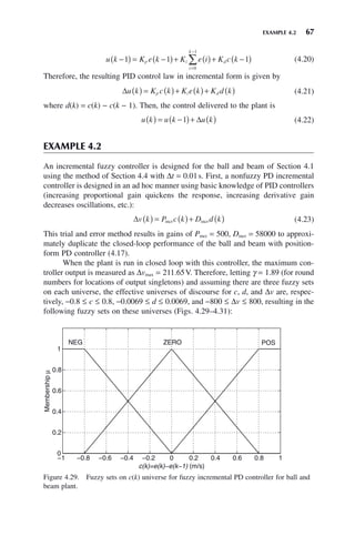
71. 4.2 TUNING FOR IMPROVED PERFORMANCE BY ADJUSTING SCALING GAINS 53
4.1.4 Defuzzification: Ball and Beam Plant
Since the output memberships are singletons (see Section 3.6.5), the crisp output of
the fuzzy controller at time t, which is the voltage input to the motor at time t, is
calculated using center average defuzzification as
v t
q e t e t
e t e t
q q
i i
i
i
i
( ) =
( ) ( )
( )
( ) ( )
( )
=
+
=
=
∑
∑
μ
μ
μ μ
,
,
1
25
1
25
9 9 10 10 14 14 15 15
9 10 14 15
+ +
+ + +
q q
μ μ
μ μ μ μ
(4.6)
where qi is the location of the membership function characterizing the singleton
fuzzy set specified in the consequent of Rule i. The crisp output of the fuzzy control-
ler for the inputs [e(t), ė(t)] = (−0.0625, 3) is
v t
( ) =
( )+ ( )+ ( )+ ( )
+ +
0 0 125 5 0 125 5 0 375 10 0 375
0 125 0 125 0 375
. . . .
. . . +
+
=
0 375
6 25
.
. V (4.7)
Thus the controller commands a clockwise rotation in order to stop the ball’s left-
ward motion. Note that the denominator in (4.7) is unity due to the partitions of
unity on the e and ė universes (Figs. 4.3 and 4.4).
4.2 TUNING FOR IMPROVED PERFORMANCE BY
ADJUSTING SCALING GAINS
As is done in many control systems both fuzzy and nonfuzzy, let us add adjustable
scaling gains g0 and g1 for inputs e and ė, respectively, and adjustable scaling gain
h for output v. These gains are used to tune the compensator to achieve better per-
formance. The closed-loop system is shown in Figure 4.9, where the contents of the
fuzzy compensator block are shown in Figure 4.10.
Figure 4.9. Closed-loop controller for ball and beam.
r(t) e(t) v(t) x(t)
Figure 4.10. Fuzzy compensator block of Figure 4.9.
e g0
g1
d
dt
g0e
g1c
h v
When the closed-loop system is simulated using a fourth-order Runge–Kutta
integration routine with a step size of Δt = 0.001s and an initial ball position of

72. 54 CHAPTER 4 FUZZY CONTROL WITH MAMDANI SYSTEMS
x(0) = −0.4m, the resulting ball movement is shown in Figure 4.11. The ball moves
toward zero, however, the response is very oscillatory. The fuzzy controller is doing
its job, but must be tuned to quicken the response and get rid of the oscillations.
This can be done by adjusting the gains g0, g1, and h.
In some cases, the fuzzy controller originally designed with all scaling gains
equaling unity may not produce a stable closed-loop system, even though the con-
troller is correctly designed according to our best judgment. In such cases, the
problem is likely that the universes of discourse are incorrectly sized for the problem.
Then it may be necessary to adjust the scaling gains initially to produce a stable
closed-loop system before the gains are further adjusted to improve the response.
Figure 4.11. Ball travel, scaling gains g0 = 1, g1 = 1, h = 1.
0 2 4 6 8 10 12 14 16 18 20
−0.4
−0.3
−0.2
−0.1
0
0.1
0.2
0.3
0.4
Time t (s)
Ball
position
(m)
Figure 4.12. Ball travel, scaling gains g0 = 1, g1 = 18, h = 1.
0 1 2 3 4 5 6 7 8 9 10
−0.4
−0.35
−0.3
−0.25
−0.2
−0.15
−0.1
−0.05
0
0.05
Time t (s)
Ball
position
(m)

73. 4.2 TUNING FOR IMPROVED PERFORMANCE BY ADJUSTING SCALING GAINS 55
When the output scaling gain h is increased to 7 while keeping g0 and g1
unchanged, the response of Figure 4.14 results.
Figure 4.13. Ball travel, scaling gains g0 = 3, g1 = 18, h = 1.
0 1 2 3 4 5 6 7 8 9 10
−0.4
−0.35
−0.3
−0.25
−0.2
−0.15
−0.1
−0.05
0
0.05
0.1
Time t (s)
Ball
position
(m)
When g1 is increased to 18 to get rid of the oscillations, the behavior shown
in Figure 4.12 results. This reduces the oscillations significantly, but the ball takes
6s to settle motionless at the center of the beam, which is too slow.
In order to quicken the response, g0 is increased to 3 while keeping g1 = 18. The
resulting response is shown in Figure 4.13. The time taken by the ball to reach the
center of the beam is significantly decreased, however, the ball overshoots its target.
Figure 4.14. Ball travel, scaling gains g0 = 3, g1 = 18, h = 7.
0 2 4 6 8 10 12
−0.4
−0.35
−0.3
−0.25
−0.2
−0.15
−0.1
−0.05
0
0.05
Time t (s)
Ball
position
(m)

74. 56 CHAPTER 4 FUZZY CONTROL WITH MAMDANI SYSTEMS
Figure 4.15. Ball travel (m) and corresponding beam angle (rad), g0 = 3, g1 = 18, h = 7.
0 0.2 0.4 0.6 0.8 1 1.2 1.4 1.6 1.8 2
−0.8
−0.6
−0.4
−0.2
0
0.2
0.4
0.6
0.8
Time t (s)
Ball position (m)
Beam angle
(rad)
This is a satisfactory response; the ball settles at the center of the beam within 1s
with no overshoot. However, note that, with h = 7, the controller now requires that
the voltage source be able to supply voltages in the range −70 ≤ v ≤ 70V at currents
demanded by the motor. If a sufficiently powerful supply is not available, it may be
necessary to accept a slower response. The control effort necessary to accomplish a
control task is always a concern in the implementation of every practical control
system.
The beam angle producing the response of Figure 4.14 is shown in
Figure 4.15. It is seen that the beam angle jumps instantaneously to an angle of
40° to achieve the rapid ball response of Figure 4.14. This may be a problem: Such
a quick movement may throw the ball off the beam! The output gain h = 7 was
chosen because values of h less then 7 result in a slower response with overshoot,
while values greater than 7 produce no significant improvement in the 1s settling
time seen in Figure 4.14.
4.3 EFFECT OF INPUT MEMBERSHIP
FUNCTION SHAPES
Let us repeat the above controller design using Gaussian input membership functions
rather than triangular. Therefore, the e and ė fuzzy sets are characterized by the
memberships in Figures 4.16 and 4.17. Note that, similar to triangular membership
functions, adjacent Gaussians may cross wherever desired. The spreads of the
Gaussians of Figures 4.16 and 4.17 have been chosen so that adjacent memberships
cross each other at 0.5.

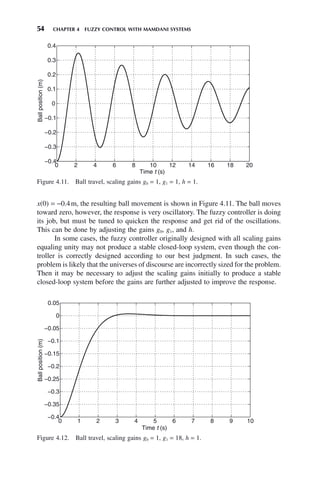
75. 4.3 EFFECT OF INPUT MEMBERSHIP FUNCTION SHAPES 57
Figure 4.16. Gaussian fuzzy sets on e universe.
−0.5 −0.25 0 0.25 0.5
0
0.2
0.4
0.6
0.8
1
e (m)
Membership
μ
NS
NL Z PS PL
Figure 4.17. Gaussian fuzzy sets on ė universe.
−4 −2 0 2 4
0
0.2
0.4
0.6
0.8
1
de/dt (m/s)
Membership
μ
NL NS Z PS PL
The rule base of Section 4.1.2 has not changed. However, the inference cal-
culation is different due to the different membership function shapes. As above,
consider a particular time t at which [e(t), ė(t)] = (−0.0625m, 3m/s). Referring to
Figure 4.16, a tracking error of e = −0.0625m is considered NL, NS, Z, PS, and PL
all to nonzero extents. Specifically, we have the following:
μe
NL
−
( ) = × −
0 0625 2 0530 10 4
. . (4.8a)
μe
NS
−
( ) =
0 0625 0 2102
. . (4.8b)
μe
Z
−
( ) =
0 0625 0 8409
. . (4.8c)

76. 58 CHAPTER 4 FUZZY CONTROL WITH MAMDANI SYSTEMS
μe
PS
−
( ) =
0 0625 0 0131
. . (4.8d)
μe
PL
−
( ) = × −
0 0625 8 0194 10 7
. . (4.8e)
Similarly, referring to Figure 4.17, ė = 3m/s is considered NL, NS, Z, PS, and
PL all to nonzero extents. Specifically, we have the following:
μ
e
NL
3 1 7764 10 15
( ) = × −
. (4.9a)
μ
e
NS
3 2 9802 10 8
( ) = × −
. (4.9b)
μ
e
Z
3 0 0020
( ) = . (4.9c)
μ
e
PS
3 0 5
( ) = . (4.9d)
μ
e
PL
3 0 5
( ) = . (4.9e)
Because all input memberships are nonzero, all 25 rules are fired to some extent.
However, the degrees of firing of most rules are very small. To avoid calculating
the degrees of firing for rules that are minimally fired, let us consider a quantity to
be in a fuzzy set only if its degree of membership in that set is at least 0.1. That is,
we consider a quantity to be in a fuzzy set only if it is in the 0.1-cut of that set.
Using this criterion, the ball position e(t) = −0.0625m qualifies as Z to an extent
0.8409, as NS to an extent 0.2102, and not as any other linguistic value on the e
universe. Similarly, the ball velocity ė(t) = 3m/s qualifies as PS to an extent 0.5, as
PL to an extent 0.5, and not as any other linguistic value on the ė universe.
Once again, rules 9, 10, 14, and 15 are on, and the rest are not fired. The
premise values of the fired rules are
μ μ μ
9 0 0625 3 0 0625 3 0 2102 0 5 0 1051
−
( ) = −
( ) ( ) = ( ) =
. , . . . .
e e
NS PS
(4.10a)
μ μ μ
10 0 0625 3 0 0625 3 0 2102 0 5 0 1051
−
( ) = −
( ) ( ) = ( ) =
. , . . . .
e e
NS PL
(4.10b)
μ μ μ
14 0 0625 3 0 0625 3 0 8409 0 5 0 4204
−
( ) = −
( ) ( ) = ( ) =
. , . . . .
e e
Z PS
(4.10c)
μ μ μ
15 0 0625 3 0 0625 3 0 8409 0 5 0 4204
−
( ) = −
( ) ( ) = ( ) =
. , . . . .
e e
Z PL
(4.10d)
The crisp output is calculated as in (4.6):
v =
( )+ ( )+ ( )+ ( )
+ +
0 0 1051 5 0 1051 5 0 4204 10 0 4204
0 1051 0 1051 0
. . . .
. . .4
4204 0 4204
6 5
+
=
.
. V (4.11)
This is similar to the crisp output calculated in (4.7) for triangular memberships. In
fact, the closed-loop behavior of the plant with Gaussian controller is very close to
that of the plant with triangular controller. This is not surprising, because the shape
of Gaussian memberships is similar to that of triangular memberships. Neither
controller is “better.” The difference is analogous to the difference that occurs when
two different people try to balance the ball on the beam by hand.
The input–output characteristic of the fuzzy controller with triangular mem-
berships is shown in Figure 4.18, and that of the controller with Gaussian member-
ships is shown in Figure 4.19. The two characteristics are essentially the same,
except for the local waves and undulations in the characteristic of Figure 4.19. These
were discussed in Section 3.6.1. These local waves are due to the curvature of the
Gaussians; they have nothing to do with the controller itself.

77. 4.4 CONVERSION OF PID CONTROLLERS INTO FUZZY CONTROLLERS 59
Figure 4.18. Input–output characteristic of fuzzy controller with triangular input
memberships, product T-norm, and singleton output fuzzy sets.
−0.5
0
0.5 −4
−2
0
2
4
−10
−5
0
5
10
de/dt
e
v
Figure 4.19. Input–output characteristic of fuzzy controller with Gaussian input
memberships, product T-norm, and singleton output fuzzy sets.
−0.5
0
0.5 −4
−2
0
2
4
−10
−5
0
5
10
de/dt
e
v
4.4 CONVERSION OF PID CONTROLLERS INTO
FUZZY CONTROLLERS
There is an exact correspondence between PID controllers and certain fuzzy control-
lers. This makes it possible to derive a fuzzy controller from a PID controller. It is
very useful to be able to do this because designing a fuzzy controller can be initially
difficult (as was seen in Sections 4.1 and 4.2). However, there exist well-known
methods of designing PID controllers (e.g., Ziegler–Nichols tuning [3]).
Even when these methods are not used, an expert can often manually adjust
a PID controller to achieve stable performance. For instance, in many applications
if the response is too sluggish, it can be quickened by increasing the proportional

78. 60 CHAPTER 4 FUZZY CONTROL WITH MAMDANI SYSTEMS
gain. Similarly, an effective strategy if the response is too oscillatory is often to
increase the derivative gain. If the steady-state error is too large, it can be reduced
by adjusting the integral gain. Using these and similar rules of thumb, an effective
PID controller can be designed for a plant relatively easily (see Section 4.2, where
these rules were used to tune the scaling gains g0 and g1). If this PID controller can
then be converted into a fuzzy controller, it may be easier to adjust the fuzzy con-
troller in a nonlinear manner to enhance robustness.
Consider a fuzzy PD controller with inputs e(t) and ė(t) and output u(t) (the
development for PI controllers and PID controllers is similar). Let the e universe of
discourse contain n symmetrical triangular fuzzy sets forming a partition of unity,
where n is odd, such that the middle triangle is centered at e = 0. Similarly, let the
ė universe contain n symmetrical triangular fuzzy sets forming a partition of unity
such that the middle triangle is centered at ė = 0. Let the u universe contain 2n − 1
equally spaced singleton fuzzy sets Q1
, … , Q2n−1
, such that the middle singleton Qn
is located at u = 0. Finally, let the rule base of the controller be specified by the
n × n rule matrix [see (4.2)]
U
Q Q Q Q
Q Q Q Q
Q Q Q Q
Q Q Q Q
ee
n
n
n
n n n n
=
⎡
⎣
+
+
+ + −
1 2 3
2 3 4 1
3 4 5 2
1 2 2 1
⎢
⎢
⎢
⎢
⎢
⎢
⎢
⎤
⎦
⎥
⎥
⎥
⎥
⎥
⎥
(4.12)
When product T-norm and center-average defuzzification are used, a fuzzy
system constructed as above exhibits a linear input–output characteristic within its
effective universe of discourse (see, e.g., Fig. 4.18). Let the effective universes of
discourse for e, ė, and u be [−emax emax], [−ėmax ėmax], and [−umax umax], respectively.
Then, the fuzzy PD controller is equivalent to the following nonfuzzy PD controller
within the fuzzy controller’s effective universe (i.e., within the linear portion of the
controller’s input–output characteristic):
u t
u
e
e t
u
e
e t
( ) = ( )+ ( )
max
max
max
max
(4.13)
Therefore, the fuzzy controller whose characteristic is shown in Figure 4.18 is
equivalent to the nonfuzzy PD controller
u t e t e t e t e t
( ) = ( )+ ( ) = ( )+ ( )
10
0 5
10
4
20 2 5
.
.
(4.14)
This suggests a method for deriving a fuzzy controller from a nonfuzzy PD
controller. Assume that we have a nonfuzzy PD controller that gives satisfactory
closed-loop behavior. In order for the equivalent fuzzy controller to be exactly equal
to the nonfuzzy PD, it is necessary that the system trajectory always remain within
the linear part of the characteristic. Therefore, with the nonfuzzy PD in operation,
measure the maximum control effort necessary to accomplish the control task. This
is the maximum absolute value of u(t) that is output by the PD in controlling the
plant. Call this umax. Then if the nonfuzzy PD controller is given by
u t K e t K e t
p d
( ) = ( )+ ( )
(4.15)

79. EXAMPLE 4.1 61
the equivalent fuzzy controller has inputs e(t), ė(t), and output u(t) with effective
universes −
⎡
⎣
⎢
⎤
⎦
⎥
γ γ
u
K
u
K
p p
max max
, , −
⎡
⎣
⎢
⎤
⎦
⎥
γ γ
u
K
u
K
d d
max max
, , and [−2γumax 2γumax], respectively.
The constant γ 1 is to guarantee the system trajectories remain within the linear
portion of the fuzzy system’s input–output characteristic. Usually γ = 2 will suffice,
but any sufficiently large γ will produce identical closed-loop behavior to the non-
fuzzy PD compensator. After the equivalent fuzzy controller has been constructed,
it can be easily altered to improve performance.
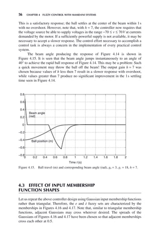
EXAMPLE 4.1
Consider the inverted pendulum plant of Figure 1.2. For simulation purposes, its
mathematical model is given by
ψ
ψ ψ ψ ψ
ψ
=
− +
( )
−
⎛
⎝
⎜
⎞
⎠
⎟
9 81
2
3
0 25
0 5
4
3
1
3
2
2
. sin cos . sin
. cos
F
(4.16)
The error e is defined as e = r(t) − ψ(t), where ψ(t) is the angle of the rod from
vertical and r(t) is a reference trajectory. Suppose it has been determined that the
PD controller
F t e t e t
( ) = − ( )+ ( )
( )
30 5 (4.17)
quickly balances the pendulum in the vertical-up position with no overshoot. Figures
4.20 and 4.21 show the rod angle response and corresponding PD controller output,
respectively for an initial rod angle of −0.1rad.
Figure 4.20. Rod angle response under nonfuzzy PD control (4.17).
0 0.2 0.4 0.6 0.8 1 1.2 1.4 1.6 1.8 2
−0.12
−0.1
−0.08
−0.06
−0.04
−0.02
0
0.02
Time t (s)
Rod
angle
ψ
(rad)

80. 62 CHAPTER 4 FUZZY CONTROL WITH MAMDANI SYSTEMS
Figure 4.21. Control effort [output of nonfuzzy PD controller (4.17)] producing response
of Figure 4.20.
0 0.2 0.4 0.6 0.8 1 1.2 1.4 1.6 1.8 2
−3
−2.5
−2
−1.5
−1
−0.5
0
0.5
Time t (s)
Control
effort
F
(N)
Figure 4.22. Fuzzy sets on e universe for equivalent fuzzy PD controller for inverted
pendulum.
−0.2 −0.1 0 0.1 0.2
0
0.2
0.4
0.6
0.8
1
e (rad)
Membership
μ
NL NS Z PS PL
From Figure 4.21, the maximum absolute value of the control effort is 3N. If
we use n = 5 fuzzy sets for e(t) and ė(t), the input and output universes given in
Figures 4.22–4.24 result.

81. EXAMPLE 4.1 63
TABLE 4.2 Tabulated Rule Base for Inverted Pendulum Controller
F
ė
NL NS Z PS PL
e
NL Q1
Q2
Q3
Q4
Q5
NS Q2
Q3
Q4
Q5
Q6
Z Q3
Q4
Q5
Q6
Q7
PS Q4
Q5
Q6
Q7
Q8
PL Q5
Q6
Q7
Q8
Q9
Figure 4.23. Fuzzy sets on ė universe for equivalent fuzzy PD controller for inverted
pendulum.
−1.2 −0.6 0 1.2
0
0.2
0.4
0.6
0.8
1
de/dt (rad/s)
Membership
μ
NL NS Z PS PL
0.6
The tabulated rule base of the controller is, from (4.12),
Figure 4.24. Fuzzy sets on F universe for equivalent fuzzy PD controller for inverted
pendulum.
−15 −10 −5 0 5 10 15
0
0.2
0.4
0.6
0.8
1
Controller output F (N)
Membership
μ
Q1 Q2
Q3
Q4
Q5
Q6
Q7
Q8
Q9

82. 64 CHAPTER 4 FUZZY CONTROL WITH MAMDANI SYSTEMS
Figure 4.25. Rod angle, 50N impulsive disturbance at t = 1.5s.
0 0.2 0.4 0.6 0.8 1 1.2 1.4 1.6 1.8 2
−5
−4
−3
−2
−1
0
1
Time t (s)
Rod
angle
ψ
(rad)
Since the nonfuzzy PD control law (4.17) is negated, the crisp output of the
fuzzy compensator should be negated as well. The performance of the inverted
pendulum in closed loop with this fuzzy PD compensator is identical to Figures 4.20
and 4.21 because the fuzzy compensator is identical to the nonfuzzy PD (4.17)
initially designed for this plant.
䊐
4.4.1 Redesign for Increased Robustness
Let the rod be balanced in the vertical-up position with the above fuzzy PD control-
ler. If the cart is bumped with an impulsive force of 50N, this disturbance is enough
to cause the rod to fall with this controller. Figure 4.25 shows this situation, where
a 50N force is applied between 1.5 and 1.55s.
The fuzzy PD can easily be redesigned on the basis of expert knowledge
so that the rod’s balance will not be destroyed by such impulsive disturbances.
The redesign consists of repositioning the output singletons so that the controller
delivers greater force when e and ė are large, but when e and ė are small the
control is unchanged. Therefore, let the new output singletons be as in Figure
4.26.
The input–output characteristic of the redesigned nonlinear fuzzy PD
controller is shown in Figure 4.27. In this figure, the characteristic of the redesigned
nonlinear fuzzy PD is the same as that of the linear controller when small control

83. EXAMPLE 4.1 65
Figure 4.26. Redesigned output singletons for fuzzy PD controller for inverted pendulum.
−40 −30 −20 −10 0 10 20 30 40
0
0.2
0.4
0.6
0.8
1
Control effort F (N)
Membership
μ
Q1
Q2
Q3
Q4
Q5
Q6
Q7
Q8
Q9
Figure 4.27. Input–output characteristics of linear PD and redesigned nonlinear fuzzy
controllers.
−0.2
−0.1
0
0.1
0.2 −2
−1
0
1
2
−30
−20
−10
0
10
20
30
de/dt (rad/s)
e (rad)
Control
effort
F
(N)
PD
controller
Fuzzy
controller
effort is required, but for cases when large control effort is required the redesigned
fuzzy controller differs significantly from the linear controller.
The response of the inverted pendulum under closed-loop control with the
redesigned nonlinear fuzzy controller is shown in Figure 4.28. In this figure, we see
that now the cart catches the rod before it falls, unlike Figure 4.25. Note that the
fuzzy PD was easily redesigned using expert knowledge to handle the impulsive
disturbance. The original nonfuzzy PD (4.17) may not be so easily redesigned to
increase robustness.

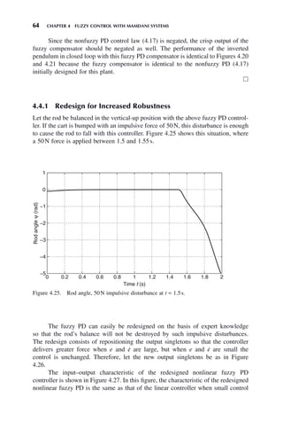
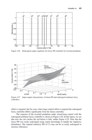
84. 66 CHAPTER 4 FUZZY CONTROL WITH MAMDANI SYSTEMS
Figure 4.28. Rod angle with 50 N impulsive disturbance at t = 1.5s, controlled with
redesigned (nonlinear) fuzzy PD controller.
0 0.5 1 1.5 2 2.5 3 3.5 4
−0.5
−0.4
−0.3
−0.2
−0.1
0
0.1
Time t (s)
Rod
angle
ψ
(radi)
The reader is reminded that all designs of fuzzy controllers done in this chapter
were done using only expert knowledge, that is, our common sense and experience
with the processes, not any control theory or knowledge of mathematical models of
the plants, which were needed only for purposes of simulation.
4.5 INCREMENTAL FUZZY CONTROL [13]
Consider the plant in Figure 4.1 with input u(t) and output y(t). So far, we have
considered only position form control laws. Position form control laws prescribe
what the control u(t) should be (i.e., u(t) = …).
An example of a position form control law is the well-known continuous-time
PID control law given by
u t K e t
T
e d T
de t
dt
i
t
d
( ) = ( )+ ( ) +
( )
⎡
⎣
⎢
⎤
⎦
⎥
∫
1
0
τ τ (4.18)
where e(t) is the summer output and K, Ti, and Td are constants chosen by the
designer. Let r(t) = r, a constant. If we sample e(t) every Δt seconds, we obtain the
discrete-time position form PID control law given by
u k K e k
t
T
e i
T
t
c k Ke k
K t
T
e i
i i
k
d
i i
( ) = ( )+ ( )+ ( )
⎡
⎣
⎢
⎤
⎦
⎥ = ( )+ ( )
= =
∑
Δ
Δ
Δ
0 0
k
k
d
p i
i
k
d
KT
t
c k
K e k K e i K c k
∑
∑
+ ( )
= ( )+ ( )+ ( )
=
Δ
0
(4.19)
where c(k) = e(k) − e(k − 1).
In incremental form control laws, the change in plant input, rather than the
inputitself,isprescribedbythecontroller.ThechangeininputisgivenbyΔu(k) = u(k) −
u(k − 1). To formulate an incremental PID control law, we need [from (4.19)]

85. EXAMPLE 4.2 67
u k K e k K e i K c k
p i
i
k
d
−
( ) = −
( )+ ( )+ −
( )
=
−
∑
1 1 1
0
1
(4.20)
Therefore, the resulting PID control law in incremental form is given by
Δu k K c k K e k K d k
p i d
( ) = ( )+ ( )+ ( ) (4.21)
where d(k) = c(k) − c(k − 1). Then, the control delivered to the plant is
u k u k u k
( ) = −
( )+ ( )
1 Δ (4.22)
EXAMPLE 4.2
An incremental fuzzy controller is designed for the ball and beam of Section 4.1
using the method of Section 4.4 with Δt = 0.01s. First, a nonfuzzy PD incremental
controller is designed in an ad hoc manner using basic knowledge of PID controllers
(increasing proportional gain quickens the response, increasing derivative gain
decreases oscillations, etc.):
Δv k P c k D d k
( ) = ( )+ ( )
incr incr (4.23)
This trial and error method results in gains of Pincr = 500, Dincr = 58000 to approxi-
mately duplicate the closed-loop performance of the ball and beam with position-
form PD controller (4.17).
When the plant is run in closed loop with this controller, the maximum con-
troller output is measured as Δvmax = 211.65V. Therefore, letting γ = 1.89 (for round
numbers for locations of output singletons) and assuming there are three fuzzy sets
on each universe, the effective universes of discourse for c, d, and Δv are, respec-
tively, −0.8 ≤ c ≤ 0.8, −0.0069 ≤ d ≤ 0.0069, and −800 ≤ Δv ≤ 800, resulting in the
following fuzzy sets on these universes (Figs. 4.29–4.31):
Figure 4.29. Fuzzy sets on c(k) universe for fuzzy incremental PD controller for ball and
beam plant.
−1 −0.8 −0.6 −0.4 −0.2 0 0.2 0.4 0.6 0.8 1
0
0.2
0.4
0.6
0.8
1
c(k)=e(k)−e(k−1) (m/s)
Membership
μ
NEG ZERO POS

86. 68 CHAPTER 4 FUZZY CONTROL WITH MAMDANI SYSTEMS
Figure 4.30. Fuzzy sets on d(k) universe for fuzzy incremental PD controller for
ball and beam plant.
−8 −6 −4 −2 0 2 4 6 8
x 10−3
0
0.2
0.4
0.6
0.8
1
d(k)=c(k)−c(k−1) (m/s2
)
Membership
μ
NEG ZERO POS
Figure 4.31. Fuzzy sets on Δv(k) universe for fuzzy incremental PD controller for
ball and beam plant.
−1000 −800 −600 −400 −200 0 200 400 600 800 1000
0
0.2
0.4
0.6
0.8
1
Δv(k) (V)
Membership
μ
NL NS Z PS PL
The rule base of the fuzzy incremental PD controller is given in tabulated form
in Table 4.3.
䊐
TABLE 4.3 Tabulated Rule Base for Incremental PD Ball and
Beam Controller
Δv
d
N Z P
c
N NL NS Z
Z NS Z PS
P Z PS PL

87. EXERCISES 69
4.6 SUMMARY
Mamdani fuzzy systems have fuzzy sets in their rule consequents, as opposed to
Takagi–Sugeno fuzzy systems (see Chapter 6), which have mathematical expres-
sions in their rule consequents. We consider the most common interconnection for
tracking: unity feedback with a fuzzy controller in casacade with the plant. Fuzzy
control is not model based, that is, its design does not depend on a mathematical
model of the plant, but on the designer’s common sense and past experience with
the process being controlled.
For the ball and beam controller (Sections 4.1–4.3), we first decide on the
inputs that would be needed (e and ė), then determine proper universes of discourse
for all inputs and outputs. These are based on our best common sense about the
system, but scaling gains are included in the design to improve performance.
Section 4.4 introduces a method for conversion of PID controllers into fuzzy
controllers. The equivalent fuzzy controller is exactly equal to the PID within its
effective universe. This technique is useful because nonfuzzy PID controllers can
be readily designed using well-known techniques. Once the equivalent fuzzy con-
troller has been obtained, it can be easily adjusted in a nonlinear manner using
heuristic knowledge to improve performance. Example 4.1 shows how this can be
done. In this example, a nonfuzzy PD controller for an inverted pendulum plant is
converted to a fuzzy controller. This fuzzy controller is then adjusted in a nonlinear
manner to increase robustness of the system to impulsive disturbances.
Section 4.5 introduces incremental fuzzy control, which prescribes the
change in input rather than the input itself. A fuzzy incremental PID is derived,
requiring inputs c(k), e(k), and d(k) where e(k) = r − y(k), c(k) = e(k) − e(k − 1), and
d(k) = c(k) − c(k − 1). In Example 4.2, the method of Section 4.4 is used to derive
an incremental fuzzy PD controller for the ball and beam plant. This controller
approximately duplicates the closed-loop performance of the position-form control-
ler derived in Section 4.1.
EXERCISES
4.1 In the fuzzy controller of Section 4.1, calculate the crisp output for an input
of (a) (e, ė) = (−0.3, 0.25); (b) (e, ė) = (−0.0625, 0.25).
4.2 Design a fuzzy controller for the ball and beam similar to the one in Section
4.1, but use 7 triangular fuzzy sets on each universe instead of 5.
4.3 Repeat Problem 4.1 for the controller of Section 4.3.
4.4 Design a fuzzy controller for the ball and beam similar to the one in Section
4.3, but use three Gaussian fuzzy sets on each universe instead of 5.
4.5 Derive a fuzzy controller equivalent to the PID controller (4.18) with K = 10,
Ti = 1, and Td = 5. The maximum control effort from the PID is 3.
4.6 Derive (4.13).
4.7 Plot the input–output characteristic of the PD controller u(t) = Kpe(t) + Kdė(t)
where Kp = Kd = 1.

88. 70 CHAPTER 4 FUZZY CONTROL WITH MAMDANI SYSTEMS
4.8 Derive the relationship between a PID and a fuzzy controller in Section
4.4, that is, that the nonfuzzy PD controller (4.15) is equivalent to a
fuzzy controller with inputs e(t) and ė(t) such that the effective
universe for e(t) is −
⎡
⎣
⎢
⎤
⎦
⎥
γ γ
u
K
u
K
p p
max max
, , the effective universe for ė(t) is
−
⎡
⎣
⎢
⎤
⎦
⎥
γ γ
u
K
u
K
d d
max max
, , and the effective universe for u(t) is [−2γumax 2γumax]
where umax is the maximum control effort required for the control task and γ
is a positive constant.
4.9 Using simulation, find a fuzzy incremental controller that balances the rod
for the inverted pendulum (Hint: Initially designing a nonfuzzy incremental
PD, then converting to fuzzy may help).
4.10 Consider the robotic link of Section 1.4 with mathematical model
ψ ψ ψ
= − − +
64 5 4
sin i
where i is the current delivered to the motor.
Design a fuzzy controller to make the link angle ψ(t) track a reference
angle r(t). Let the inputs to the controller be ψ,
ψ and the output be the
motor current i(t). (a) Define three fuzzy sets Negative (N), Zero (Z),
and Positive (P) on each universe. (b) Write the rule base for your controller.
(c) Simulate the closed-loop system for an initial condition of
ψ ψ
π
, ,
[ ]=
⎡
⎣
⎢
⎤
⎦
⎥
2
0 and a reference signal of
r t t
( ) = +
π
π
2
sin
Use a fourth order Runge–Kutta integration routine with a step size of 0.001s.

89. 71
Fuzzy Control and Identification, By John H. Lilly
Copyright © 2010 John Wiley Sons, Inc.
Basic fuzzy control, unlike most control methods, is not based on a mathematical
model of the process being controlled. This is one of the strengths of fuzzy control.
However, more advanced fuzzy control methods, such as some types of parallel
distributed compensation and fuzzy adaptive control, as well as fuzzy system
identification, do require at least an assumption of some particular structure of the
model. Some methods assume continuous-time linear or nonlinear state-space model
structures while others assume discrete-time state space or input–output difference
equation model structures.
We emphasize that a particular dynamic system can be modeled with any of
these model structures, as will be demonstrated below. The particular structure used
depends on the one required by the control or identification method. Therefore, we
give a brief summary of several well-known model structures for dynamic systems.
5.1 CONTINUOUS-TIME MODEL FORMS
The four most common methods for describing continuous-time dynamic systems
are the transfer function (for time-invariant linear systems), the impulse response
(for time-varying or time-invariant linear systems), the input–output ordinary dif-
ferential equation (for any type of continuous-time system), and the state-space
description (for any type of system). Of these, only the linear or nonlinear time-
invariant state-space descriptions are useful for fuzzy identification and control. Now
we give brief summaries of these model structures.
5.1.1 Nonlinear Time-Invariant Continuous-Time
State-Space Models
Let x(t) = [x1, x2, … , xn] be the vector of states of a time-invariant continuous-time
nth order single-input, single-output nonlinear system with input u(t) and output y(t).
A very general form for the system model is
MODELING AND CONTROL
METHODS USEFUL FOR
FUZZY CONTROL
CHAPTER 5

90. 72 CHAPTER 5 MODELING AND CONTROL METHODS USEFUL FOR FUZZY CONTROL
x F x u
= ( )
, (5.1a)
y H x u
= ( )
, (5.1b)
where F(x, u) and H(x, u) are continuously differentiable functions of their
arguments.
If (5.1) can be put in the form
x f x g x u
= ( )+ ( ) (5.2a)
y h x
= ( ) (5.2b)
it is said to be feedback linearizable (a mathematically rigorous definition of
feedback linearizability is more involved [1]. This means that it can be linearized
by an appropriately designed feedback law. Under certain assumptions, by differen-
tiating the output it is possible to transform (5.2) into the so-called companion
form [21]:
y x x u
m
( )
= ( )+ ( )
δ η (5.3)
where y(m)
= dm
y/dtm
. The integer m is known as the relative degree of the system.
If m n, there can be zero dynamics ([1,21,22]), which are assumed stable in this
book.
Models of the form (5.3) are used in indirect adaptive fuzzy control algorithms.
In such algorithms, the system model is not known in advance; rather it is identified
in this form using one of several fuzzy identification schemes (gradient, least squares,
etc.) (see Chapter 9).
EXAMPLE 5.1
Consider the forced rigid pendulum shown in Figure 5.1. It has a massless shaft of
length L with a mass M concentrated at the end, and a coefficient of friction B at
the attach point. The external torque applied to the shaft at the attach point is τ. This
is a version of the motor-driven robotic link of Section 1.4.
Figure 5.1. Forced rigid pendulum.
B
L
M

91. EXAMPLE 5.1 73
The rotational version of Newton’s second law gives ϒ = I
ψ , where ψ is the
angle of the shaft from vertical, I is the moment of inertia of the pendulum about
the attach point, and ϒ is the sum of all torques acting on the shaft. Thus, the math-
ematical model of this system is
τ ψ ψ ψ
− − =
B MgL I
sin
where I = ML2
and g is the acceleration of gravity. Let M = 1kg, L = 1m, B =
1kg-m/s2
and g = 9.81m/s2
. If we define the states x1 = ψ and x2 =
ψ , the output
y = ψ, and the input u = τ, the following state and output equations result:
x x
1 2
= (5.4a)
x x x u
2 1 2
9 8
= − − +
. sin (5.4b)
y x
= 1 (5.4c)
This is in the form of (5.1) with x = [x1 x2]T
,
F x u
F
F
x
x x u
,
. sin
( ) =
⎡
⎣
⎢
⎤
⎦
⎥ =
− − +
⎡
⎣
⎢
⎤
⎦
⎥
1
2
2
1 2
9 8
(5.5)
and
H x u x
,
( ) = 1
The right-hand sides of (5.4a) and (5.4b) can be rewritten to give
x
x
x
x x
u
1
2
2
1 2
9 8
0
1
⎡
⎣
⎢
⎤
⎦
⎥ =
− −
⎡
⎣
⎢
⎤
⎦
⎥ +
⎡
⎣
⎢
⎤
⎦
⎥
. sin
(5.6a)
y x
= 1 (5.6b)
Since this is the form of (5.2) with f x
x
x x
( ) =
− −
⎡
⎣
⎢
⎤
⎦
⎥
2
1 2
9 8
. sin
, g x
( ) =
⎡
⎣
⎢
⎤
⎦
⎥
0
1
, and
h(x) = x1, the system is feedback linearizable.
Differentiating (5.6b) once, we have ẏ = ẋ1(= x2). This is not in the form of
(5.3) because there is no u term present. Differentiating the output once again, we
have ÿ = ẋ2. Then, the model can be expressed in the form of (5.3) with relative
degree m = 2, δ(x) = −9.8sinx1 − x2 and η(x) = 1:
y x x u
= − − +
9 8 1 2
. sin (5.7)
The Matlab code to simulate the pendulum model (5.4) forced with an input
torque of
u
t t
t
=
( ) ≤
⎧
⎨
⎩
2 2 2
0 2
sin ,
,
π s
s
(5.8)
is in the Appendix . The resulting pendulum angle is shown in Figure 5.2.

92. 74 CHAPTER 5 MODELING AND CONTROL METHODS USEFUL FOR FUZZY CONTROL
5.1.2 Linear Time-Invariant Continuous-Time
State-Space Models
Let the nonlinear system be modeled as in (5.1). Assume x = 0, u = 0 is an equilib-
rium point of the system [i.e., F(0, 0) = 0]. Then expanding F(x, u) in a Taylor series
about x = 0, u = 0, we have
F x u F
F
x
x
F
u
u
x
u
x
u
, ,
( ) = ( )+
∂
∂
+
∂
∂
+
=
=
=
=
0 0
0
0
0
0
…
In this series, the higher-order terms (i.e., those involving higher than first powers
of x or u or cross-products between these) can be ignored in the vicinity of the
equilibrium point because these terms are vanishingly small in this region. Therefore,
in the vicinity of x = 0, u = 0, the system is approximately described by the linear
model
x t Ax t bu t
( ) = ( )+ ( ) (5.9a)
y t cx t
( ) = ( ) (5.9b)
where A
F
x x
u
=
∂
∂ =
=
0
0
, b
F
u x
u
=
∂
∂ =
=
0
0
, and c
H
x x
u
=
∂
∂ =
=
0
0
EXAMPLE 5.2
The model of the forced pendulum of Example 5.1 can be expressed as (5.1) with
F(x, u) as in (5.5). Then,
Figure 5.2. Pendulum angle, full nonlinear model (5.1).
0 1 2 3 4 5 6 7 8 9 10
−0.1
−0.05
0
0.05
0.1
0.15
−0.15
Time (s)
Pendulum
angle
ψ
(rad)

93. 5.2 MODEL FORMS FOR DISCRETE-TIME SYSTEMS 75
∂
∂
=
∂
∂
∂
∂
∂
∂
∂
∂
⎡
⎣
⎢
⎢
⎢
⎢
⎤
⎦
⎥
⎥
⎥
⎥
=
−
=
=
=
=
F
x
F
x
F
x
F
x
F
x
x
u
x
u
0
0
1
1
1
2
2
1
2
2 0
0
0 1
9. cos .
8 1
0 1
9 8 1
1 0
0
x x
u
−
⎡
⎣
⎢
⎤
⎦
⎥ =
− −
⎡
⎣
⎢
⎤
⎦
⎥
=
=
∂
∂
=
∂
∂
∂
∂
⎡
⎣
⎢
⎢
⎢
⎢
⎤
⎦
⎥
⎥
⎥
⎥
=
⎡
⎣
⎢
⎤
⎦
⎥
=
=
=
=
F
u
F
u
F
u
x
u
x
u
0
0
1
2
0
0
0
1
This gives the model (5.9) linearized about the equilibrium point x1 = 0, x2 = 0,
u = 0:
x t x t u t
( ) =
− −
⎡
⎣
⎢
⎤
⎦
⎥ ( )+
⎡
⎣
⎢
⎤
⎦
⎥ ( )
0 1
9 8 1
0
1
.
(5.10a)
y t x t
( ) = [ ] ( )
1 0 (5.10b)
When (5.10) is simulated with the input torque of (5.8), the behavior of
the linearized system is almost identical to that of the original nonlinear system
(5.4). This occurs because ψ(t) and
ψ t
( ) remain close to their equilibrium
values of ψ = 0,
ψ = 0 , hence higher-order terms in the Taylor series are negligibly
small.
5.2 MODEL FORMS FOR DISCRETE-TIME SYSTEMS
Most systems to be controlled are continuous-time systems. If such a system is to
be controlled by connecting it to a digital computer, which is virtually always the
case with fuzzy control, the control input must eventually be represented in discrete-
time form, necessitating some type of method that approximates continuous-time
signals by discrete-time signals. This could be done by calculating the continuous-
time control signal from a continuous-time model in the form of (5.1), (5.3), or
(5.9) and then discretizing it, or by calculating a discrete-time control signal from
a discrete-time model of the system. In the former case, the approximation error
is the result of discretizing a continuous-time control signal. In the latter case, the
error is the result of approximating a continuous-time system by a discrete-time
system.
If the system is discrete time, either inherently or through sampling, all signals
are considered as existing only at discrete time instants, kΔt, where k = 0, 1, 2, …
and Δt is the sampling interval for sampled continuous-time systems. If the
system is inherently discrete, Δt = 1. For sampled continuous-time systems, the
sampling interval Δt is usually supressed, that is, x(kΔt) is written x(k).
In this section, we give two forms of discrete-time models for linear
systems.

94. 76 CHAPTER 5 MODELING AND CONTROL METHODS USEFUL FOR FUZZY CONTROL
5.2.1 Input–Output Difference Equation Model for Linear
Discrete-Time Systems
One common method of describing the input–output behavior of a discrete-time
linear system is by an input–output difference equation involving present and past
inputs and outputs. This is known as an autoregressive moving average (ARMA)
model. The general form of ARMA model used in this book is
y k q y k q u k
+
( ) = ( ) ( )+ ( ) ( )
− −
1 1 1
α β (5.11)
with
α q a a q a q
n
n
− − − −
( )
( ) = + + +
1
1 2
1 1
(5.12a)
β q b b q b q
m
m
− − −
( ) = + + +
1
0 1
1
(5.12b)
where k is an integer representing time, u(k) is the system input at time k, y(k) is the
system output at time k, ai, i = 1, 2, … , n and bj, j = 0, 1, … , m are constants, and
q−1
is the backward-shift operator defined by
q y k y k
−
( ) = −
( )
1
1 (5.13)
By incrementing the time index in (5.11) by n − 1, the following model results:
y k n a y k n a y k n a y k
b u k n b u k n
n
+
( )− + −
( )− + −
( )− − ( )
= + −
( )+ + −
(
1 2
0 1
1 2
1 2
)
)+ + + − −
( )
b u k n m
m 1 (5.14)
Implementing the forward-shift operator q in (5.13) results in
q y k a q y k a q y k a y k
b q u k b q u k
n n n
n
n n
( )− ( )− ( )− − ( )
= ( )+ (
− −
− −
1
1
2
2
0
1
1
2
)
)+ + ( )
− −
b q u k
m
n m 1
from which we can write the system pulse transfer function:
y k
u k
b q b q b q
q a q a q a
n n
m
n m
n n n
n
( )
( )
=
+ + +
− − − −
− − − −
− −
0
1
1
2 1
1
1
2
2
(5.15)
5.2.2 Linear Time-Invariant Discrete-Time
State-Space Models
If we define the states x1(k) = y(k), x2(k) = y(k + 1), x3(k) = y(k + 2), … ,
xn(k) = y(k + n − 1) in (5.14), the following state equations result
x k Ax k bu k
+
( ) = ( )+ ( )
1 (5.16a)
y k cx k
( ) = ( ) (5.16b)
where x(k) = [x1(k) x2(k) … xn(k)]T
and

95. EXAMPLE 5.3 77
A
a a a a
b
n n n
=
⎡
⎣
⎢
⎢
⎢
⎢
⎢
⎢
⎤
⎦
⎥
⎥
⎥
⎥
⎥
⎥
=
− −
0 1 0 0
0 0 1 0
0 0 0
1
0
0
0
1 2 1
,
1
1
0
0
⎡
⎣
⎢
⎢
⎢
⎢
⎢
⎢
⎤
⎦
⎥
⎥
⎥
⎥
⎥
⎥
=
⎡
⎣
⎢
⎢
⎢
⎢
⎢
⎢
⎤
⎦
⎥
⎥
⎥
⎥
⎥
⎥
, c b
b
T
m
The above gives a method for converting from input–output difference equa-
tion form to linear discrete-time state-space form. It is also possible to convert to
linear discrete-time state-space form directly from linear continuous-time state space
form (5.9). To do this, discretize time and define x(k) = x(kΔt), where Δt is the
sample time and k is an integer. Approximate ẋ as
x
x k x k
t
≈
+
( )− ( )
1
Δ
Then (5.9) becomes
x k x k
t
Ax k bu k
+
( )− ( )
≈ ( )+ ( )
1
Δ
y k cx k
( ) = ( )
which yields
x k I A t x t b tu k
+
( ) = +
( ) ( )+ ( )
1 Δ Δ
y k cx k
( ) = ( )
EXAMPLE 5.3
Consider the linearized continuous-time model of the forced pendulum (5.10).
If the sampling time Δt is 0.01s, the discrete-time linearized model of the forced
pendulum is
x k x k u k
+
( ) =
−
⎡
⎣
⎢
⎤
⎦
⎥ ( )+
⎡
⎣
⎢
⎤
⎦
⎥ ( )
1
1 0 01
0 098 0 99
0
0 01
.
. . .
(5.17a)
y k x k
( ) = [ ] ( )
1 0 (5.17b)
䊐
The Matlab code to simulate the pendulum model (5.17) forced with the input
torque of (5.8) is given in the Appendix. The behavior of the linearized discrete-time
system is nearly identical to that of the original nonlinear system. This is because
the sampling time Δt = 0.01s is small enough that all signals are essentially constant
over one sampling interval.

96. 78 CHAPTER 5 MODELING AND CONTROL METHODS USEFUL FOR FUZZY CONTROL
EXAMPLE 5.4
Applying the forward shift operator (5.13) to (5.17) yields
qx k x k u k
( ) =
−
⎡
⎣
⎢
⎤
⎦
⎥ ( )+
⎡
⎣
⎢
⎤
⎦
⎥ ( )
1 0 01
0 098 0 99
0
0 01
.
. . .
y k x k
( ) = [ ] ( )
1 0
Solving for x(k) in the first equation and substituting this into the second equation
yields
y k qI u k
( ) = [ ] −
−
⎡
⎣
⎢
⎤
⎦
⎥
⎛
⎝
⎜
⎞
⎠
⎟
⎡
⎣
⎢
⎤
⎦
⎥ ( )
−
1 0
1 0 01
0 098 0 99
0
0 01
1
.
. . .
Therefore, the pulse transfer function of the forced pendulum is
y k
u k q q
( )
( )
=
− +
0 0001
1 99 0 991
2
.
. .
which gives rise to the linear input–output difference equation in the form of (5.11)
describing the forced pendulum:
y k y k y k u k
+
( ) = ( )− −
( )+ −
( )
1 1 99 0 991 1 0 0001 1
. . . (5.18)
The Matlab code to simulate the pendulum model (5.18)) forced with the input
torque of (5.8) is given in the Appendix . The behavior of the system (5.18) is
essentially identical to that of the original nonlinear system.
It should be emphasized that the models (5.4), (5.7), (5.10), (5.17), and (5.18)
all describe the forced pendulum under certain conditions. Each is inaccurate in its
own way. The original nonlinear model (5.4) is perhaps the least inaccurate, but
even it is still only an approximation of the true physical pendulum. This is due to
several reasons: (1) Equation (5.4) assumes the pendulum shaft is massless and that
the mass M is concentrated at one point at the end of the shaft. This is not true for
an actual pendulum. (2) Equation (5.4) assumes that the shaft is absolutely rigid. In
an actual pendulum, the shaft is flexible to some extent. (3) Equation (5.4) assumes
that the quantities M, B, and L are precisely known. In reality, they are only approxi-
mately known, and B may change over time. (4) The input torque τ is not known
with precision. If the difficulties (1–4) listed above were not present, that is, if an
absolutely accurate model were used to describe the pendulum, it would be impos-
sibly complex. This gives support for using the various models above, since all
mathematical models are inaccurate to some extent.
5.3 SOME CONVENTIONAL CONTROL METHODS
USEFUL IN FUZZY CONTROL
The advent of Takagi–Sugeno (T–S) fuzzy systems ([8,9,11,12,23–25]) has enabled
the use of some well-known conventional control methods for control of nonlinear

97. 5.3 SOME CONVENTIONAL CONTROL METHODS USEFUL IN FUZZY CONTROL 79
systems with unknown models. Below we give the methods that will be used in later
chapters in conjunction with T–S fuzzy systems.
5.3.1 Pole Placement Control [26]
If the system model is of the linear time-invariant state-space form [(5.9) for
continuous-time systems or (5.16) for discrete-time systems], properties like stabil-
ity, rise time, settling time, overshoot, and so on, of the system depend on the sys-
tem’s poles, which are the eigenvalues of the dynamic matrix A. If the eigenvalues
are not as desired, they can be moved to desired locations via full state feedback if
the system is controllable, that is, if
C = [ ]
−
b Ab A b A b
n
2 1
(5.19)
is nonsingular. The matrix C is called the controllability matrix.
Let the characteristic polynomial of A be
λ λ λ λ
I A d d d
n
n
n
− = + + + +
−
−
1
1
1 0
(5.20)
The eigenvalues of A are the roots of this polynomial. The full-state feedback control
law is
u t kx t
( ) = − ( ) (5.21)
When this input is applied to system (5.9), the resulting closed-loop system is
x t A bk x t
( ) = −
( ) ( ) (5.22)
Let the desired closed-loop eigenvalues be μ1, μ2, … , μn. These are the desired
eigenvalues of A − bk. Then the desired characteristic polynomial of A − bk is
λ μ λ μ λ μ λ δ λ δ λ δ
−
( ) −
( ) −
( ) = + + + +
−
−
1 2 1
1
1 0
n
n
n
n
(5.23)
Define
W
d d d
d d
d
n
n
=
⎡
⎣
⎢
⎢
⎢
⎢
⎢
⎢
⎤
⎦
⎥
⎥
⎥
⎥
⎥
⎥
−
−
1 2 1
2 3
1
1
1 0
1 0 0
1 0 0 0
(5.24)
Then the full-state feedback control law that places the closed-loop poles at μ1,
μ2, … , μn is given by (5.21), where
k d d d d T
n n n n
= − − − −
[ ]
− − − −
−
δ δ δ δ
0 0 1 1 2 2 1 1
1
, , , ,
(5.25)
with
T W
= C (5.26)
Note that this method applies for discrete-time systems like (5.16) as well.

98. 80 CHAPTER 5 MODELING AND CONTROL METHODS USEFUL FOR FUZZY CONTROL
EXAMPLE 5.5
Consider the linear continuous-time time-invariant system given by (5.9) with
A b
=
−
−
−
⎡
⎣
⎢
⎢
⎢
⎢
⎤
⎦
⎥
⎥
⎥
⎥
=
−
⎡
⎣
⎢
⎢
⎢
⎢
⎤
⎦
⎥
⎥
⎥
⎥
1 0 1 0
0 2 1 1
0 0 0 1
0 1 1 0
1
0
0
1
,
Design a linear state feedback control law u = −kx such that the poles of the closed-
loop system are −1, −1 + j, −1 − j, −2.
Solution: The characteristic polynomial of A is
λ λ λ λ λ
I A
− = − − + +
4 3 2
4 3
This can also be found using the Matlab command poly. Then, we have d0 = 3,
d1 = 1, d2 = −4, d3 = −1 and
W =
− −
− −
−
⎡
⎣
⎢
⎢
⎢
⎢
⎤
⎦
⎥
⎥
⎥
⎥
1 4 1 1
4 1 1 0
1 1 0 0
1 0 0 0
The controllability matrix of the system is
C = [ ]=
−
− −
− − −
⎡
⎣
⎢
⎢
⎢
⎢
⎤
⎦
⎥
⎥
⎥
⎥
b Ab A b A b
2 3
1 1 0 0
0 1 1 4
0 1 0 2
1 0 2 1
Therefore,
T W
= =
− −
−
−
−
⎡
⎣
⎢
⎢
⎢
⎢
⎤
⎦
⎥
⎥
⎥
⎥
C
5 3 2 1
1 0 1 0
2 1 1 0
0 2 1 1
The desired closed-loop characteristic polynomial is
λ λ λ λ λ λ λ λ
+
( ) + −
( ) + +
( ) +
( ) = + + + +
1 1 1 2 5 10 10 4
4 3 2
j j
This can also be found using the Matlab command poly. Then we have δ0 = 4,
δ1 = 10, δ2 = 10, δ3 = 5. Then, from (5.25), the feedback matrix k is
k T
= [ ] = −
[ ]
−
1 9 14 6 0 41 21 6
1

99. EXAMPLE 5.6 81
and the feedback control law is
u kx x x x
= − = − − +
41 21 6
2 3 4 (5.27)
To check, verify that the eigenvalues of A − bk are −1, −1 + j, −1 − j, −2 as desired.
䊐
If the number of states is small (say n ≤ 3), it may be easier to calculate k by
simply calculating the characteristic polynomial of A − bk with variable k and equat-
ing this to the desired closed-loop characteristic polynomial.
EXAMPLE 5.6
Consider the discrete-time linear time-invariant system given by (5.16) with
A b
=
−
⎡
⎣
⎢
⎤
⎦
⎥ =
⎡
⎣
⎢
⎤
⎦
⎥
0 1 1 5
1 2 0
0
1
. .
.
,
Design a linear state feedback control law u = −kx such that the poles of the closed-
loop system are 0.8 ± j0.2.
Solution: Since this is only a two-state system, we can find k by calculating
the characteristic polynomial of A − bk with variable k and equating this to the
desired closed-loop characteristic polynomial. The desired characteristic polyno-
mial is
λ λ λ λ
− −
( ) − +
( ) = − +
0 8 0 2 0 8 0 2 1 6 0 68
2
. . . . . .
j j (5.28)
If k = [k1 k2], the closed-loop characteristic polynomial is
λ
λ
λ
λ λ
I A bk
k k
k k k
− + =
−
− + +
= + −
( ) + − − +
(
0 1 1 5
1 2
0 1 1 5 0 1 1 8
1 2
2
2 1 2
. .
.
. . . . )
) (5.29)
Equating coefficients in (5.28) and (5.29) yields k2 − 0.1 = −1.6 and
−1.5k1 − 0.1k2 + 1.8 = 0.68, from which k1 = 0.8467 and k2 = −1.5. Thus the feed-
back control law that places the closed-loop eigenvalues at 0.8 ± j0.2 is
u kx x x
= − = − +
0 8467 1 5
1 2
. . (5.30)
5.3.2 Tracking Control [27]
Assume that an nth-order SISO linear discrete-time system has unit delay (a similar
development applies for systems with delays 1). Then it has an input–output
ARMA model as in (5.11) and (5.12).
The one-step-ahead tracking control problem is to find a control u(k) that
brings the output at time k + 1(y(k + 1)) to some desired bounded value r(k + 1) and
is such that y(k) = r(k) thereafter. It is easy to verify that the control that accom-
plishes this satisfies

100. 82 CHAPTER 5 MODELING AND CONTROL METHODS USEFUL FOR FUZZY CONTROL
β α
q u k r k q y k
− −
( ) ( ) = +
( )− ( ) ( )
1 1
1 (5.31)
To see this, substitute (5.31) into (5.11). The resulting closed-loop system has
bounded inputs and outputs provided that the poles of the inverse model (i.e., the
zeros of the polynomial qm
β(q−1
) lie inside the unit circle. This design procedure
applies to n-step-ahead tracking problems with obvious modifications.
EXAMPLE 5.7
Consider a linear time-invariant discrete-time system described by the second-order
input–output difference equation:
y k y k k u k u k
+
( ) = ( )− −
( )+ ( )+ −
( )
1 1 5 0 4 1 0 6 1
. . . (5.32)
Find a control u(k) that brings the output at time k + 1 to the desired reference signal
r(k) = 0.1sin(0.1πk).
Solution: The system can be rewritten as (5.11) with α(q−1
) = 1.5 − 0.4q−1
and
β(q−1
) = 1 + 0.6q−1
. Note that this system is unstable because the polynomial
q2
[1 − q−1
α(q−1
)] = q2
− 1.5q + 0.4 has roots outside the unit circle. Also, we are
assured the tracking objective can be accomplished with a bounded control because
the poles of the inverse model [i.e., the zeros of the polynomial qβ(q−1
)] are inside
the unit circle.
The control law (5.31) yields the one-step-ahead tracking controller:
u k u k y k y k k
( ) = − −
( )− ( )+ −
( )+ +
( )
( )
0 6 1 1 5 0 4 1 0 1 0 1 1
. . . . sin . π (5.33)
5.3.3 Model Reference Control [27]
The objective of model reference control is to find a plant input such that the output
of the controlled system tracks that of a reference model. The following development
is a generalization of the tracking controller above. Let the plant be described by
the input–output ARMA model (5.11) and (5.12). A similar development applies for
systems with delays greater than 1.
Assume, without loss of generality, that the desired output y*(k) satisfies
the following reference model:
E q y k q gH q r k
− − −
( ) ( ) = ( ) ( )
1 1 1
* (5.34)
where g is a constant gain, r(k) is an arbitrary bounded input, and
H q h q h q
l
l
− − −
( )= + + +
1
1
1
1 (5.35a)
E q e q e q
l
l
− − −
( )= + + +
1
1
1
1 (5.35b)
The associated pulse transfer function of the reference model is

101. EXAMPLE 5.8 83
G q
y k
r k
q gH q
E q
−
− −
−
( )=
( )
( )
=
( )
( )
1
1 1
1
*
(5.36)
The model reference control problem is to find a control u(k) that brings the plant
output y(k) to the output y*(k) of the reference model (5.34) excited by a known
bounded signal r(k).
The control u(k) that accomplishes y(k) = y*(k) satisfies
γ β
q y k q u k gH q r k
− − −
( ) ( )+ ( ) ( ) = ( ) ( )
1 1 1
(5.37)
where γ(q−1
) is the unique polynomial of order n − 1 satisfying
E q q q q
− − − −
( )= + ( )− ( )
[ ]
1 1 1 1
1 γ α (5.38)
To see this, realize that from (5.38) we have
γ α
q q E q q
− − −
( )= ( )−
[ ]+ ( )
1 1 1
1
Substituting this in (5.37) yields
qE q y k y k q y k q u k gH q r k
− − − −
( ) ( )− +
( )+ ( ) ( )+ ( ) ( ) = ( ) ( )
1 1 1 1
1 α β
Since the plant model is given by (5.11), this reduces to (5.34).
EXAMPLE 5.8
Consider a system described by the ARMA model:
y k y k y k u k u k
+
( ) = ( )− −
( )+ ( )+ −
( )
1 0 4 1 8 1 1 2 1
. . .
Let the desired reference signal obey (5.36) with g = 2 and
H q q
− −
( )= +
1 1
1 0 3
.
E q q q
− − −
( )= + +
1 1 2
1 0 5 0 5
. .
Find a control u(k) that brings the plant output to the output of the reference model
(5.36) excited by a known bounded signal r(k).
Solution: This system is in the form of (5.11) with α(q−1
) = 0.4 − 1.8q−1
and
β(q−1
) = 1.2 + q−1
. Note that the system is unstable because the polynomial
q2
[1 − q−1
α(q−1
)] = q2
− 0.4q + 1.8 has roots outside the unit circle. Also, we are
assured that the tracking objective can be accomplished with a bounded control
because the poles of the inverse model (i.e., the zeros of the polynomial qβ(q−1
))
are inside the unit circle.
The model pulse transfer function is
G q
q q
q q
−
− −
− −
( )=
+
+ +
1
1 2
1 2
2 0 6
1 0 5 0 5
.
. .

102. 84 CHAPTER 5 MODELING AND CONTROL METHODS USEFUL FOR FUZZY CONTROL
The identity (5.38) is given by
1 0 5 0 5 1 0 4 1 8
1 2 1 2 1
0 1
1
+ +
( )= − + + +
( )
− − − − − −
. . . .
q q q q q q
γ γ
Therefore, we have
γ γ γ
q q q
− − −
( )= + = −
1
0 1
1 1
0 9 1 3
. .
and control u(k) that accomplishes model following obeys (5.37):
0 9 1 3 1 2 2 1 0 3
1 1 1
. . . .
−
( ) ( )+ +
( ) ( ) = +
( ) ( )
− − −
q y k q u k q r k
This yields the model reference control law:
u k u k y k y k r k r k
( ) = − −
( )− ( )+ −
( )+ ( )+ −
( )
[ ]
1
1 2
1 0 9 1 3 1 2 0 6 1
.
. . .
䊐
5.3.4 Feedback Linearization
Let the plant be modeled as in (5.3). Assume further that η(x(t)) ≥ η0 0, so that
the system is controllable for all t. Let the control law be
u t
x t
x t v t
( ) =
( )
( )
− ( )
( )+ ( )
( )
1
η
δ (5.39)
where v(t) is an arbitrary function of t chosen to produce a stable closed-loop system
with desired characteristics.
Then, combining (5.3) and (5.39), the closed-loop system is given by:
y x t x t
x t
x t v t
m
( )
= ( )
( )+ ( )
( )
( )
( )
− ( )
( )+ ( )
( )
⎡
⎣
⎢
⎤
⎦
⎥
δ η
η
δ
1
or
y v t
m
( )
= ( ) (5.40)
This is a linear system with input v(t). Thus the nonlinear system has been linearized
by the feedback (5.39).
EXAMPLE 5.9
For the system (5.3), let the input be given by (5.39) with
v t a y a y a y b r b r b r
m m
m
m m
m
( ) = − − − − + + + +
−
( ) −
( ) −
( ) −
( )
1
1
2
2
1
1
2
2
(5.41)
where a1 … am and b1 … bm are arbitrary constants chosen by the designer and r(t)
is an external input. Then the closed-loop system is linear with transfer function:

103. 5.4 SUMMARY 85
Y s
R s
b s b s b
s a s a s a
m m
m
m m m
m
( )
( )
=
+ + +
+ + + +
− −
− −
1
1
2
2
1
1
2
2
Thus by choice of a1 … am and b1 … bm, any desired closed-loop performance
(overshoot, rise time, steady-state response, etc.) may be obtained.
EXAMPLE 5.10
Consider the forced pendulum (5.4). Find a feedback control law so that the closed-
loop system is linear with unity zero-frequency gain and poles at s = −1 ± j.
Solution: The desired transfer function (unity zero-frequency gain, poles at
s = −1 ± j) is
ψ
τ
s
s s s
( )
( )
=
+ +
2
2 2
2
Considering the model (5.7), which is equivalent to (5.4), we have
δ ψ ψ ψ ψ
, . sin
( ) = − −
9 8 and η ψ ψ
,
( ) = 1.
Then by (5.39) and (5.41) the necessary control law is
τ ψ ψ ψ ψ ψ ψ ψ
= + − − + = − − +
9 8 2 2 2 9 8 2 2
. sin . sin
r r (5.42)
where r(t) is the external input to the system. The block diagram of the closed-loop
system is shown in Figure 5.3.
Figure 5.3. Block diagram of forced pendulum (5.4) with feedback linearizing control
(5.42).
2
2
9.8 sin
Forced
pendulum
r(t) t
y
y
5.4 SUMMARY
This chapter contains model forms and control methodologies that are useful for
fuzzy control. All of these will be used in various fuzzy control strategies imple-
mented with T–S fuzzy systems in the following chapters. The presentation is brief,
that is, some familiarity with controls is assumed. However, the theory has been

104. 86 CHAPTER 5 MODELING AND CONTROL METHODS USEFUL FOR FUZZY CONTROL
kept to a minimum, with the assumption that if more detail is desired, the reader can
consult one of the references given in the chapter.
The model forms considered for continuous-time systems are the continuous-
time nonlinear state equations (5.1), continuous-time linear state equations
(5.9), and the feedback-linearization form (5.3). The model forms considered for
discrete-time systems are the discrete-time linear state equations (5.16) and
input–output difference equation, or ARMA model (5.11).
Continuous-time nonlinear state equations are not used directly for fuzzy
control, but are used to derive models in feedback-linearizeable form. Feedback-
linearizable model forms are used in indirect adaptive control schemes for adaptive
model following (Section 5.3.4). Continuous- and discrete-time linear state equation
model forms are used in parallel distributed compensators for pole placement
(Section 5.3.1). Input–output difference equation models are used in tracking and
model reference controllers (Sections 5.3.2 and 5.3.3).
EXERCISES
5.1 Put the inverted pendulum of Example 4.1 in feedback linearizable form (5.3).
Consider the output to be the rod angle ψ.
5.2 Put the inverted pendulum of Example 4.1 in linearized continuous-time
state-space form (5.9).
5.3 Consider the linear continuous-time state-space system (5.9) with
A b c
=
− − −
⎡
⎣
⎢
⎢
⎢
⎤
⎦
⎥
⎥
⎥
=
⎡
⎣
⎢
⎢
⎢
⎤
⎦
⎥
⎥
⎥
= −
[ ]
0 1 0
0 0 1
1 3 2
0
0
1
1 1 0
, ,
Put the system in discrete-time state-space form (5.16). Let the sample time
be Δt = 0.01s.
5.4 Consider the linear discrete-time system (5.16) with
A b c
=
− −
⎡
⎣
⎢
⎢
⎢
⎤
⎦
⎥
⎥
⎥
=
⎡
⎣
⎢
⎢
⎢
⎤
⎦
⎥
⎥
⎥
= −
[ ]
0 1 0
0 0 1
0 1 0 0 2
0
0
1
1 1 0
. .
, ,
Put the system in input–output difference equation form (5.11).
5.5 Consider a system described by the input–output difference equation
y k y k y k u k u k
+
( ) = ( )− −
( )+ ( )+ −
( )
1 0 3 0 6 1 1 5 1
. . .
Put the system in discrete-time state-space form (5.16).
5.6 Consider the system described by the linear continuous-time state-space
equations given in Problem 5.3. Find a linear state feedback law (5.21)
to place the closed-loop poles at −1, −1 + j, and −1 − j. Use the method of
Example 5.5.

105. EXERCISES 87
5.7 Repeat Problem 6 using the method of Example 5.6.
5.8 Consider a system described by the input–output difference equation
y k y k y k u k u k
+
( ) = ( )− −
( )+ ( )+ −
( )
1 0 4 1 8 1 1 2 1
. . .
Design a one-step-ahead tracking controller to make the system’s output track
the reference signal r(k) = 0.1(1 − cos(0.3k)).
5.9 For the system of Problem 5.8, design a model reference controller to
make the system’s output track the output of the model whose transfer func-
tion is
G q
q q
q q
−
− −
− −
( )=
+
+ +
1
1 2
1 2
0 2
1 0 6 0 7
.
. .
with the input r(k) = 0.1(1 − cos(0.3k)).
5.10 Consider the system in feedback-linearizeable form
y x x x x u
= + + +
( )
1
2
2 3
2
2
1 sin
Design a feedback control law for this system so that the closed-loop system
is linear with transfer function
Y s
R s
s
s s s
( )
( )
=
+
+ + +
2
3 2
1
2 2 1
where r(t) is an external input.

106. 88
Fuzzy Control and Identification, By John H. Lilly
Copyright © 2010 John Wiley Sons, Inc.
Takagi–Sugeno (T–S) fuzzy systems are more general than the Mamdani fuzzy
systems discussed in Chapters 3 and 4. In fact, it can be shown that Mamdani
systems are special cases of T–S fuzzy systems. The T–S systems are important
because they enable a kind of control called parallel distributed control, they facili-
tate fuzzy identification of dynamic systems and adaptive fuzzy control, and they
enable stability proofs for certain closed-loop systems involving fuzzy controllers.
Their drawback is that they are less intuitive than Mamdani systems.
In T–S systems, the consequents of the rules do not involve fuzzy sets as do
Mamdani systems, but instead are mathematical expressions. The mathematical
expressions can be any linear functions of any variables. In this book, we consider only
consequents that are either memoryless affine functions of the fuzzy system’s inputs,
or one of the linear dynamic system model forms discussed in Sections 5.1 or 5.2. In
the former case, the T–S fuzzy system performs an interpolation between memoryless
functions. In the latter case, the T–S system performs an interpolation between
dynamic systems. The latter case is useful for fuzzy identification and control.
6.1 TAKAGI–SUGENO FUZZY SYSTEMS AS
INTERPOLATORS BETWEEN MEMORYLESS
FUNCTIONS
Consider a T–S fuzzy system with R rules of the form:
R x P x P x P q f
i
K L
n n
M i
i
If is and is and and is then
1 1 2 2 i
, = ( ) (6.1)
The input universes X1, X2, … , Xn are as before, with various fuzzy sets defined on
them, but now the consequents are memoryless functions fi (•). The crisp output of
this system is
y
q x
x
i
i
i
R
i
i
R
crisp
=
( )
( )
=
=
∑
∑
μ
μ
1
1
(6.2)
TAKAGI–SUGENO FUZZY
SYSTEMS
CHAPTER 6

107. EXAMPLE 6.1 89
where μi(x) is the premise membership value of Rule i. The crisp output can be
expressed as
y q t q t q t
R
R
crisp
= ( )+ ( )+ + ( )
1
1
2
2
ξ ξ ξ
(6.3)
where
ξ
μ
μ
i
i
j
j
R
t
x t
x t
i R
( ) =
( )
( )
( )
( )
=
=
∑
1
1, ,
…
(6.4)
are called fuzzy basis functions [28].
In this section, we assume the functions fi(•) are affine functions of the
inputs:
f a a x a x a x
i
i i i
n
i
n
i
( ) = + + + +
0 1 1 2 2 (6.5)
where the coefficients aj
i
are constants. The output ycrisp
is a nonlinear function of
the inputs x1, … , xn.
EXAMPLE 6.1
Consider a two-input T–S fuzzy system with rules
1. If x1 is P1
1
and x2 is P2
1
, then q1
= 1 + x1 + x2.
2. If x1 is P1
1
and x2 is P2
2
, then q2
= 2x1 + x2.
3. If x1 is P1
2
and x2 is P2
1
, then q3
= −1 + x1 − 2x2.
4. If x1 is P1
2
and x2 is P2
2
, then q4
= −2 − x1 + 0.5x2.
Inside the effective universe of discourse the fuzzy sets P1
1
, P1
2
, P2
1
, and P2
2
are char-
acterized by the following membership functions:
μ1
1
1
1
2
1
2
1
0 8493
x
x
( ) = −
+
⎛
⎝
⎜
⎞
⎠
⎟
⎡
⎣
⎢
⎤
⎦
⎥
exp
.
μ1
2
1
1
2
1
2
1
0 8493
x
x
( ) = −
−
⎛
⎝
⎜
⎞
⎠
⎟
⎡
⎣
⎢
⎤
⎦
⎥
exp
.
μ2
1
2
2
2
1
2
1
0 8493
x
x
( ) = −
+
⎛
⎝
⎜
⎞
⎠
⎟
⎡
⎣
⎢
⎤
⎦
⎥
exp
.
μ2
2
2
2
2
1
2
1
0 8493
x
x
( ) = −
−
⎛
⎝
⎜
⎞
⎠
⎟
⎡
⎣
⎢
⎤
⎦
⎥
exp
.
These are shown in Figures 6.1 and 6.2.

108. 90 CHAPTER 6 TAKAGI–SUGENO FUZZY SYSTEMS
Given the crisp input (x1, x2), the crisp output of this system is [see (6.3), (6.4)]:
y x x q x x x x
i
i
i
crisp
1 2 1 2 1 2
1
4
, , ,
( ) = ( ) ( )
=
∑ ξ
where ξ μ μ
i i j
j
x x x x x x
1 2 1 2 1 2
1
4
, , ,
( ) = ( ) ( )
=
∑ , i = 1, 2, 3, 4 and, assuming product
T-norm,
μ1 1 2
1
2
2
1
2
1
0 8493
1
2
1
0 8493
x x
x x
, exp
.
exp
.
( ) = −
+
⎛
⎝
⎜
⎞
⎠
⎟
⎡
⎣
⎢
⎤
⎦
⎥ −
+
⎛
⎝
⎜
⎞
⎞
⎠
⎟
⎡
⎣
⎢
⎤
⎦
⎥
2
(6.6a)
Figure 6.2. Memberships for x2 input.
−1.5 −1 −0.5 0 0.5 1 1.5
0
0.2
0.4
0.6
0.8
1
x2
μ
P2
1
P2
2
Figure 6.1. Memberships for x1 input.
−1.5 −1 −0.5 0 0.5 1 1.5
0
0.2
0.4
0.6
0.8
1
x1
μ
P1
1
P1
2

109. 6.1 TAKAGI–SUGENO FUZZY SYSTEMS AS INTERPOLATORS BETWEEN MEMORYLESS FUNCTIONS 91
μ2 1 2
1
2
2
1
2
1
0 8493
1
2
1
0 8493
x x
x x
, exp
.
exp
.
( ) = −
+
⎛
⎝
⎜
⎞
⎠
⎟
⎡
⎣
⎢
⎤
⎦
⎥ −
−
⎛
⎝
⎜
⎞
⎞
⎠
⎟
⎡
⎣
⎢
⎤
⎦
⎥
2
(6.6b)
μ3 1 2
1
2
2
1
2
1
0 8493
1
2
1
0 8493
x x
x x
, exp
.
exp
.
( ) = −
−
⎛
⎝
⎜
⎞
⎠
⎟
⎡
⎣
⎢
⎤
⎦
⎥ −
+
⎛
⎝
⎜
⎞
⎞
⎠
⎟
⎡
⎣
⎢
⎤
⎦
⎥
2
(6.6c)
μ4 1 2
1
2
2
1
2
1
0 8493
1
2
1
0 8493
x x
x x
, exp
.
exp
.
( ) = −
−
⎛
⎝
⎜
⎞
⎠
⎟
⎡
⎣
⎢
⎤
⎦
⎥ −
−
⎛
⎝
⎜
⎞
⎞
⎠
⎟
⎡
⎣
⎢
⎤
⎦
⎥
2
(6.6d)
For the particular crisp input (x1, x2) = (0.6, −0.3), we calculate μ1(0.6,
−0.3) = 0.1207, μ2(0.6, −0.3) = 0.0525, μ3(0.6, −0.3) = 0.6373, and μ4(0.6,
−0.3) = 0.2774. These values yield the following fuzzy basis function values:
ξ1 0 6 0 3 0 1207 0 1207 0 0525 0 6373 0 2774 0 1110
. , . . . . . . .
−
( ) = + + +
( ) =
ξ2 0 6 0 3 0 0525 0 1207 0 0525 0 6373 0 2774 0 0483
. , . . . . . . .
−
( ) = + + +
( ) =
ξ3 0 6 0 3 0 6373 0 1207 0 0525 0 6373 0 2774 0 5858
. , . . . . . . .
−
( ) = + + +
( ) =
ξ4 0 6 0 3 0 2774 0 1207 0 0525 0 6373 0 2774 0 2550
. , . . . . . . .
−
( ) = + + +
( ) =
The consequent functions are evaluated for (x1, x2) = (0.6, −0.3) as
q1
0 6 0 3 1 0 6 0 3 1 3
. , . . . .
−
( ) = + − =
q2
0 6 0 3 2 0 6 0 3 0 9
. , . . . .
−
( ) = ( )− =
q3
0 6 0 3 1 0 6 2 0 3 0 2
. , . . . .
−
( ) = − + − −
( ) =
q4
0 6 0 3 2 0 6 5 0 3 2 75
. , . . . . .
−
( ) = − − + −
( ) = −
Therefore, the crisp output of the T–S fuzzy system corresponding to the input
(x1, x2) = (0.6, −0.3) is
ycrisp
0 6 0 3 1 3 0 1110 0 9 0 0483 0 2 0 5858 2 75 0
. , . . . . . . . .
−
( ) = ( )+ ( )+ ( )− .
.
2550
0 3962
( )
= −
The characteristic surface of the fuzzy system is shown in Figure 6.3. This
was found by evaluating the crisp output corresponding to numerous points in the
domain −2 ≤ x1 2, −2 ≤ x2 2. The surface is an interpolation between the four
affine planar functions q1
(x1, x2), q2
(x1, x2), q3
(x1, x2), and q4
(x1, x2). Small portions
of these planes are shown on the corresponding edges of the characteristic surface
of Figure 6.3. It is seen that on the appropriate edges of the surface, the planes match
well with the surface. For instance, if x1 and x2 are both large negative numbers (i.e.,
x1 −1, x2 −1), Rule 1 would be fired with certainty, while Rules 2, 3, and 4 would
be fired very little. Therefore, the crisp output of the fuzzy system would be essen-
tially q1
.
Referring to Figure 6.3, in the area of the surface where both x1 and x2 are
between −1 and −2, the surface is indeed essentially equal to q1
. Inside the effective
universe of discourse (i.e., −1 ≤ x1 1, −1 ≤ x2 1), the fuzzy system interpolates
between the planes.

110. 92 CHAPTER 6 TAKAGI–SUGENO FUZZY SYSTEMS
6.2 TAKAGI–SUGENO FUZZY SYSTEMS AS
INTERPOLATORS BETWEEN CONTINUOUS-TIME
LINEAR STATE-SPACE DYNAMIC SYSTEMS
Consider a T–S fuzzy system with R rules of the form:
Ri: If x1(t) is PK
1 and x2(t) is PL
2 and … and xn(t) is Pn
M
, then
x t A x t b u t
i
i i
( ) = ( )+ ( ) (6.7)
The contents of the n × 1 vector x(t) = [x1(t), x2(t), … , xn(t)]T
are the system states
that vary continuously with time t. The input universes X1, X2, … , Xn are as before,
with various fuzzy sets defined on them, but now the consequents are continuous-
time linear constant-coefficient dynamic systems involving the states. The quantities
Ai and bi are n × n and n × 1 constant-coefficient matrices, respectively, for i = 1,
2, … , n. This fuzzy system does not have a single crisp output, rather it produces
a time-varying system described by the differential equation:
x t
x t A x t b u t
x t
i i i
i
R
i
i
R
( ) =
( )
( ) ( )+ ( )
( )
( )
( )
=
=
∑
∑
μ
μ
1
1
(6.8)
or
x t A t x t b t u t
( ) = ( ) ( )+ ( ) ( ) (6.9)
where A(t) = ξ1(t)A1 + ξ2(t)A2 + … + ξR(t)AR and b(t) = ξ1(t)b1 + ξ2(t)b2 + … +
ξR(t)bR and ξi(t), i = 1, … , R are the fuzzy basis functions described in (6.4).
Matrices A(t) and b(t) contain functions of the system states, making the system
(6.9) a nonlinear time-varying system.
Figure 6.3. Characteristic surface of the T–S fuzzy system with individual consequents
plotted at appropriate corners.
−2
−1
0
1
2
−2
−1
0
1
2
−5
0
5
x1
x2
y
crisp
q1
q4
q
3
q2

111. EXAMPLE 6.2 93
Figure 6.4. Memberships for fuzzy sets on x1 universe.
−1.5 −1 −0.5 0 0.5 1 1.5
0
0.2
0.4
0.6
0.8
1
x1
μ
P1
1
P1
2
EXAMPLE 6.2
Consider a two-input T–S fuzzy system with rules
1. If x1(t) is P1
1
and x2(t) is P2
1
, then ẋ1
(t) = A1x(t) + b1u(t).
2. If x1(t) is P1
1
and x2(t) is P2
2
, then ẋ2
(t) = A2x(t) + b2u(t).
3. If x1(t) is P1
2
and x2(t) is P2
1
, then ẋ3
(t) = A3x(t) + b3u(t).
4. If x1(t) is P1
2
and x2(t) is P2
2
, then ẋ4
(t) = A4x(t) + b4u(t).
where A1
0 1
2 2
=
− −
⎡
⎣
⎢
⎤
⎦
⎥ , b1
0
2
=
⎡
⎣
⎢
⎤
⎦
⎥ , A2
0 1
1 2
=
− −
⎡
⎣
⎢
⎤
⎦
⎥ , b2
2
2
=
⎡
⎣
⎢
⎤
⎦
⎥
A b A b
3 3 4 4
0 1
3 2
2
2
1 1
2 2
0
2
=
− −
⎡
⎣
⎢
⎤
⎦
⎥ =
−
⎡
⎣
⎢
⎤
⎦
⎥ =
− −
⎡
⎣
⎢
⎤
⎦
⎥ =
−
⎡
⎣
⎢
⎤
⎦
⎥
, , ,
The fuzzy sets P1
1
, P1
2
, P2
1
, and P2
2
are characterized by the membership functions
shown in Figures 6.4 and 6.5.
For an arbitrary input (x1, x2) inside the effective universe of discourse
(i.e., −1 ≤ x1 1, −1 ≤ x2 1), the premise values for the above four rules are
calculated as:
μ1 1 2
0 5 0 5 0 25 0 5
t x t x t
( ) = − ( )+
( ) − ( )+
( )
. . . . (6.10a)
μ2 1 2
0 5 0 5 0 25 0 5
t x t x t
( ) = − ( )+
( ) ( )+
( )
. . . . (6.10b)
μ3 1 2
0 5 0 5 0 25 0 5
t x t x t
( ) = ( )+
( ) − ( )+
( )
. . . . (6.10c)
μ4 1 2
0 5 0 5 0 25 0 5
t x t x t
( ) = ( )+
( ) ( )+
( )
. . . . (6.10d)
where we have used the equations of the membership functions in Figures 6.4 and
6.5 inside the effective universes and product T-norm.

112. 94 CHAPTER 6 TAKAGI–SUGENO FUZZY SYSTEMS
If we consider a particular instant of time t1 at which x1(t1) = 0.4 and
x2(t1) = −0.8, we have the following premise values for the rules: μ1(t1) = 0.21,
μ2(t1) = 0.09, μ3(t1) = 0.49, and μ4(t1) = 0.21. These yield the following basis func-
tion values:
ξ1 1 0 21 0 21 0 09 0 49 0 21 0 21
t
( ) = + + +
( ) =
. . . . . .
ξ2 1 0 09 0 21 0 09 0 49 0 21 0 09
t
( ) = + + +
( ) =
. . . . . .
ξ3 1 0 49 0 21 0 09 0 49 0 21 0 49
t
( ) = + + +
( ) =
. . . . . .
ξ4 1 0 21 0 21 0 09 0 49 0 21 0 21
t
( ) = + + +
( ) =
. . . . . .
Here we see the advantage of partitions of unity on the input universes combined
with product T-norms: in the calculation of ycrisp
, the denominator, which is the sum
of the premise values of all rules, always equals unity. As a result, the basis func-
tions ξi are merely the premise values μi, saving computer resources to calculate
them.
The system at time t1 is described by the state-space differential equation
x t A t x t b t u t
( ) = ( ) ( )+ ( ) ( )
1 1
where
A t t A t A t A t A
( ) = ( ) + ( ) + ( ) + ( )
=
− −
⎡
⎣
⎢
⎤
⎦
⎥ +
ξ ξ ξ ξ
1 1 1 2 1 2 3 1 3 4 1 4
0 21
0 1
2 2
. 0 09
0 1
1 2
0 49
0 1
3 2
0 21
1 1
2 2
0 21 1
. . .
.
− −
⎡
⎣
⎢
⎤
⎦
⎥ +
− −
⎡
⎣
⎢
⎤
⎦
⎥ +
− −
⎡
⎣
⎢
⎤
⎦
⎥
=
−2 4 2
. −
⎡
⎣
⎢
⎤
⎦
⎥
Figure 6.5. Memberships for fuzzy sets on x2 universe.
−2 −1 0 1 2
0
0.2
0.4
0.6
0.8
1
x2
μ
P2
1
P2
2

113. 6.3 DISCRETE-TIME LINEAR STATE-SPACE DYNAMIC SYSTEMS 95
Figure 6.6 State trajectories of T–S fuzzy system that interpolates four linear continuous-
time constant-coefficient state-space systems, Example 6.2.
0 1 2 3 4 5 6 7 8
−4
−3
−2
−1
0
1
2
3
Time t (s)
States
x1
(t)
x2
(t)
and
b t t b t b t b t b
1 1 1 1 2 1 2 3 1 3 4 1 4
0 21
0
2
0 0
( ) = ( ) + ( ) + ( ) + ( )
=
⎡
⎣
⎢
⎤
⎦
⎥ +
ξ ξ ξ ξ
. . 9
2
2
0 49
2
2
0 21
0
2
0 8
1 16
⎡
⎣
⎢
⎤
⎦
⎥ +
−
⎡
⎣
⎢
⎤
⎦
⎥ +
−
⎡
⎣
⎢
⎤
⎦
⎥ =
−
⎡
⎣
⎢
⎤
⎦
⎥
. .
.
.
To summarize, the system at time t1 is described by
x
x
x
x
u
1
2
1
2
0 21 1
2 4 2
0 8
1 16
⎡
⎣
⎢
⎤
⎦
⎥ =
− −
⎡
⎣
⎢
⎤
⎦
⎥
⎡
⎣
⎢
⎤
⎦
⎥ +
−
⎡
⎣
⎢
⎤
⎦
⎥
.
.
.
.
Note that this describes the system at only one time t1. As t changes, A(t) and b(t)
change.
A simulation of this system was carried out using fourth-order Runge–Kutta
integration with a step size of Δt = 0.01s. An input of u(t) = 3sin(πt) with initial
condition x1(0) = x2(0) = 0 yields the state trajectories shown in Figure 6.6. The
nonlinear nature of the system can be seen in this response. The Matlab simulation
program producing Figure 6.6 is given in the Appendix.
6.3 TAKAGI–SUGENO FUZZY SYSTEMS AS
INTERPOLATORS BETWEEN DISCRETE-TIME LINEAR
STATE-SPACE DYNAMIC SYSTEMS
T–S fuzzy systems can be used to create time-varying discrete-time state-space
dynamic systems. Consider a T–S fuzzy system with R rules of the form:

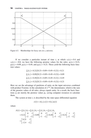
114. 96 CHAPTER 6 TAKAGI–SUGENO FUZZY SYSTEMS
Ri: If x1(k) is PK
1 and x2(k) is PL
2 and … and xn(k) is Pn
M
, then
x k A x k b x k
i
i i
+
( ) = ( )+ ( )
1 . (6.11)
The contents of the n × 1 vector x(k) = [x1(k), x2(k), … , xn(k)]T
are the system
states that vary with the discrete time k ∈ {0, 1, 2, 3, …}. The input universes X1,
X2, … , Xn are as before, with various fuzzy sets defined on them, but now the
consequents are discrete-time linear constant-coefficient state-space systems. This
fuzzy system does not have a single crisp output, rather it produces a time-varying
system described by the state-space difference equation:
x k
k A x k b x k
k
i i i
i
R
i
i
R
+
( ) =
( ) ( )+ ( )
( )
( )
=
=
∑
∑
1 1
1
μ
μ
(6.12)
or
x k A k x k b k u k
+
( ) = ( ) ( )+ ( ) ( )
1 (6.13)
where A(k) = ξ1(k)A1 + ξ2(k)A2 + … + ξR(k)AR and b(k) = ξ1(k)b1 + ξ2(k)b2 + … +
ξR(k)bR with fuzzy basis functions
ξ
μ
μ
i
i
j
j
R
k
k
k
( ) =
( )
( )
=
∑
1
(6.14)
As k varies, the states x(k) also vary. Therefore, the fuzzy basis functions and the
matrices A(k) and b(k) vary with time. Matrices A(k) and b(k) contain functions of
the system states, making the system (6.13) a nonlinear time-varying system.
EXAMPLE 6.3
Consider a two-input T–S fuzzy system with rules
1. If x1(k) is P1
1
and x2(k) is P2
1
, then x1
(k + 1) = A1x(k) + b1u(k).
2. If x1(k) is P1
1
and x2(k) is P2
2
, then x2
(k + 1) = A2 x(k) + b2u(k).
3. If x1(k) is P1
2
and x2(k) is P2
1
, then x3
(k + 1) = A3 x(k) + b3u(k).
4. If x1(k) is P1
2
and x2(k) is P2
2
, then x4
(k + 1) = A4 x(k) + b4u(k).
where A1
0 1 0
0 2 0 2
=
−
⎡
⎣
⎢
⎤
⎦
⎥
.
. .
, b1
0
1
=
⎡
⎣
⎢
⎤
⎦
⎥ , A2
0 0 1
1 0 2
=
−
⎡
⎣
⎢
⎤
⎦
⎥
.
.
, b2
0 1
1
=
⎡
⎣
⎢
⎤
⎦
⎥
.
A b A b
3 3 4 4
0 3 1
0 0 2
0 1
1
0 1 1
0 2 0 5
0
=
−
⎡
⎣
⎢
⎤
⎦
⎥ =
−
⎡
⎣
⎢
⎤
⎦
⎥ =
⎡
⎣
⎢
⎤
⎦
⎥ =
.
.
,
.
,
.
. .
,
−
−
⎡
⎣
⎢
⎤
⎦
⎥
1
Let the fuzzy sets P1
1
, P1
2
, P2
1
, and P2
2
be characterized by the Gaussian membership
functions shown in Figures 6.1 and 6.2. Then for an arbitrary input (x1, x2) and

115. EXAMPLE 6.3 97
product T-norm, the premise values for the above four rules are calculated as
in (6.6).
If we consider a particular instant of time k1 at which x1(k1) = 0.4 and
x2(k1) = −0.8, the instantaneous fuzzy basis function values are
ξ
μ
μ
1 1
1 1
1
1
4
0 25
0 25 0 0272 0 7578 0 0825
0 2
k
k
k
i
i
( ) =
( )
( )
=
+ + +
=
=
∑
.
. . . .
. 237
ξ
μ
μ
2 1
2 1
1
1
4
0 0272
0 25 0 0272 0 7578 0 0825
0
k
k
k
i
i
( ) =
( )
( )
=
+ + +
=
=
∑
.
. . . .
.
.0243
ξ
μ
μ
3 1
3 1
1
1
4
0 7578
0 25 0 0272 0 7578 0 0825
0
k
k
k
i
i
( ) =
( )
( )
=
+ + +
=
=
∑
.
. . . .
.
.6782
ξ
μ
μ
4 1
4 1
1
1
4
0 0825
0 25 0 0272 0 7578 0 0825
0
k
k
k
i
i
( ) =
( )
( )
=
+ + +
=
=
∑
.
. . . .
.
.0738
Then the system at time k1 is described by the difference equation
x k A k x k b k u k
+
( ) = ( ) ( )+ ( ) ( )
1 1 1
where
A k k A k A k A k A
1 1 1 1 2 1 2 3 1 3 4 1 4
0 2237
0 1 0
0 2 0
( ) = ( ) + ( ) + ( ) + ( )
=
−
ξ ξ ξ ξ
.
.
. .2
0 0243
0 0 1
1 0 2
0 6782
0 3 1
0 0 2
0 073
⎡
⎣
⎢
⎤
⎦
⎥ +
−
⎡
⎣
⎢
⎤
⎦
⎥ +
−
⎡
⎣
⎢
⎤
⎦
⎥
+
.
.
.
.
.
.
. 8
0 1 1
0 2 0 5
0 1737 0 7544
0 0056 0 2124
.
. .
. .
. .
⎡
⎣
⎢
⎤
⎦
⎥ =
−
−
⎡
⎣
⎢
⎤
⎦
⎥
and
b k k b k b k b k b
1 1 1 1 2 1 2 3 1 3 4 1 4
0 2237
0
1
0
( ) = ( ) + ( ) + ( ) + ( )
=
⎡
⎣
⎢
⎤
⎦
⎥ +
ξ ξ ξ ξ
. . . .
.
.
0243
1
1
0 6782
1
1
0 0738
0
1
0 06538
0 8
⎡
⎣
⎢
⎤
⎦
⎥ +
−
⎡
⎣
⎢
⎤
⎦
⎥ +
−
⎡
⎣
⎢
⎤
⎦
⎥ =
−
5
524
⎡
⎣
⎢
⎤
⎦
⎥
To summarize, the system at time k1 is described by
x k
x k
x k
1
2
1
1
1
0 1737 0 7544
0 0056 0 2124
+
( )
+
( )
⎡
⎣
⎢
⎤
⎦
⎥ =
−
−
⎡
⎣
⎢
⎤
⎦
⎥
( )
. .
. . x k
u k
2
0 06538
0 8524
( )
⎡
⎣
⎢
⎤
⎦
⎥ +
−
⎡
⎣
⎢
⎤
⎦
⎥ ( )
.
.
Note that this describes the system at only one time k1. As k changes, A(k) and b(k)
change.
This system was simulated with x1(0) = x2(0) = 0, a sampling time of Δt = 0.2s,
and u(t) = 3sin(πt), where t = kΔt and k is an integer. The resulting state trajectories

116. 98 CHAPTER 6 TAKAGI–SUGENO FUZZY SYSTEMS
are shown in Figure 6.7. The nonlinear nature of the system can be seen in this
response. The Matlab simulation program producing Figure 6.7 is given in the
Appendix.
6.4 TAKAGI–SUGENO FUZZY SYSTEMS AS
INTERPOLATORS BETWEEN DISCRETE-TIME DYNAMIC
SYSTEMS DESCRIBED BY INPUT–OUTPUT DIFFERENCE
EQUATIONS
The above method can be used to create a nonlnear time-varying discrete-time
dynamic system described by an input–output difference equation. This form of
system model is particularly useful when system identification techniques are being
used because an unknown system is often identified in the form of a discrete-time
input–output difference equation rather than state-space equations as above. If state-
space equations are desired (e.g., for parallel distributed pole placement), they can
always be obtained from input–output difference equations via well-known canoni-
cal forms.
Consider a T–S fuzzy system with R rules of the form:
R y k P y k P y k n P
y k
i
K L
n
M
i
: ,
If is and is and and is then
( ) −
( ) − +
( )
+
1 2
1 1
1
…
(
( ) = ( )+ −
( )+ + − +
( )+
( )+ −
( )
α α α
β β
i i i n
i i
y k y k y k n
u k u k
, , ,
, ,
1 2
1 2
1 1
1
+ + − +
( )
βi mu k m
, 1
(6.15)
where y(k), … , y(k − n + 1), are present and past plant outputs and u(k), … ,
u(k − m + 1) are present and past plant inputs. This way of describing a discrete-
time system is commonly used in system identification techniques.
Figure 6.7. Input and corresponding states for discrete-time system created by a four-rule
T–S fuzzy system.
0 1 2 3 4 5 6 7 8 9
−1
−0.8
−0.6
−0.4
−0.2
0
0.2
0.4
Time t (s)
States
x1(t)
x2(t)

117. EXAMPLE 6.4 99
This fuzzy system produces a time-varying discrete-time system described by
the difference equation:
y k
y k y k n y k
y k y k n
i
i
i
R
i
i
+
( ) =
( ) − +
( )
( ) +
( )
( ) − +
( )
( )
=
∑
1
1 1
1
1
μ
μ
, ,
, ,
…
…
=
=
∑
1
R
(6.16)
where μi(y(k), … , y(k − n + 1)) is the premise membership value of Rule i.Therefore,
the discrete-time system produced by the T–S fuzzy system is
y k y k y k y k n
u k u k u k
n
m
+
( ) = ( )+ −
( )+ + − +
( )+
( )+ −
( )+ +
1 1 1
1
1 2
1 2
α α α
β β β
− +
( )
m 1
(6.17)
where
α α ξ α ξ α ξ
1 1 1 1 2 1 2 1
= ( )+ ( )+ + ( )
, , ,
k k k
R R
α α ξ α ξ α ξ
2 1 2 1 2 2 2 2
= ( )+ ( )+ + ( )
, , ,
k k k
R R
α α ξ α ξ α ξ
n n n R n R
k k k
= ( )+ ( )+ + ( )
1 1 2 2
, , ,
β β ξ β ξ β ξ
1 1 1 1 2 1 2 1
= ( )+ ( )+ + ( )
, , ,
k k k
R R
β β ξ β ξ β ξ
2 1 2 1 2 2 2 2
= ( )+ ( )+ + ( )
, , ,
k k k
R R
β β ξ β ξ β ξ
m m m R m R
k k k
= ( )+ ( )+ + ( )
1 1 2 2
, , ,
and the fuzzy basis functions are given by
ξ
μ
μ
j
j
i
i
R
k
k
k
j R
( ) =
( )
( )
=
=
∑
1
1
, , ,
…
EXAMPLE 6.4
Consider a two-input T–S fuzzy system with rules
1. If y(k) is P1
1
and y(k − 1) is P2
1
, then
y k y k y k u k u k
1
1 0 5 0 5 1 0 6 1
+
( ) = ( )− −
( )+ ( )+ −
( )
. . . .
2. If y(k) is P1
1
and y(k − 1) is P2
2
, then
y k y k y k u k u k
2
1 0 4 0 8 1 1 2 1
+
( ) = ( )− −
( )+ ( )− −
( )
. . . .
3. If y(k) is P1
2
and y(k − 1) is P2
1
, then
y k y k y k u k u k
3
1 0 2 0 5 1 1 5 0 7 1
+
( ) = ( )+ −
( )+ ( )− −
( )
. . . . .
4. If y(k) is P1
2
and y(k − 1) is P2
2
, then
y k y k y k u k u k
4
1 0 8 0 6 1 1 5 1
+
( ) = ( )− −
( )− ( )+ −
( )
. . . .

118. 100 CHAPTER 6 TAKAGI–SUGENO FUZZY SYSTEMS
Let the fuzzy sets P1
1
, P1
2
, P2
1
, and P2
2
be characterized by the Gaussian
membership functions shown in Figures 6.1 and 6.2. Then for an arbitrary input
(x1, x2) the premise values for the above four rules (μi, i = 1, … , 4) are calculated
as in (6.6).
If we consider a particular instant of time k1 at which y(k1) = 0.4 and
y(k1 − 1) = −0.8, the instantaneous fuzzy basis function values are the same as in
Example 6.3. Then the system at time k1 is described by the input-output difference
equation
y k k y k k y k k u k k u k
+
( ) = ( ) ( )+ ( ) −
( )+ ( ) ( )+ ( ) −
( )
1 1 1
1 1 2 1 1 1 2 1
α α β β
where
α ξ ξ ξ ξ
1 1 1 1 2 1 3 1 4 1
0 5 0 4 0 2 0 8 0 3163
k k k k k
( ) = ( )+ ( )+ ( )+ ( ) =
. . . . .
α ξ ξ ξ ξ
2 1 1 1 2 1 3 1 4 1
0 5 0 8 0 5 0 6 0 1635
k k k k k
( ) = − ( )− ( )+ ( )− ( ) =
. . . . .
β ξ ξ ξ ξ
1 1 1 1 2 1 3 1 4 1
1 1 2 1 5 1 5 1 1595
k k k k k
( ) = ( )+ ( )+ ( )− ( ) =
. . . .
β ξ ξ ξ ξ
2 1 1 1 2 1 3 1 4 1
0 6 1 0 7 1 0 2911
k k k k k
( ) = ( )− ( )− ( )+ ( ) = −
. . .
To summarize, the system at time k1 is described by
y k y k y k u k u k
+
( ) = ( )+ −
( )+ ( )− −
( )
1 0 3163 0 1635 1 1 1595 0 2911 1
. . . .
Note that this describes the system at only one time k1. As k changes, α1, α2, β1, and
β2 also change. A simulation of this system with a sampling time of Δt = 1s,
y(0) = y(−1) = 0, and u(t) = sin(0.05πt), where t = kΔt yields the trajectory shown
in Figure 6.8. The nonlinear nature of the system can be seen in this response. The
Matlab program producing Figure 6.8 is given in the Appendix.
Figure 6.8. Output of T–S fuzzy system that interpolates four linear constant-coefficient
discrete-time dynamic systems to produce a nonlinear discrete-time dynamic system.
0 10 20 30 40 50 60
−2
−1.5
−1
−0.5
0
0.5
1
Time t (s)
Input
u(t)
and
output
y
(t)
u(t)
y(t)

119. EXERCISES 101
6.5 SUMMARY
This chapter introduces Takagi–Sugeno (T–S) fuzzy systems, which are generaliza-
tions of Mamdani fuzzy systems (Chapter 3). The consequents of T–S systems are
general mathematical functions rather than fuzzy sets. T–S fuzzy systems make
identification of nonlinear systems (Chapter 9) possible, as well as adaptive fuzzy
control (Chapter 10). They also enable stability proofs for closed-loop systems
controlled by T–S fuzzy controllers (Chapter 7).
The three types of T–S fuzzy systems considered in this book are those with
consequents that are (1) affine functions, (2) normal form state-space models, or (3)
input–output difference equation models.
If the consequents are affine functions, the T–S fuzzy system realizes a static
nonlinear function, as in Example 6.1 and Figure 6.3. It was seen that this type of
fuzzy system interpolates the hyperplanes in the individual consequents inside the
effective universe of discourse. This type of fuzzy system will be utilized in Chapters
9 and 10 to identify nonlinear plants in the form of (5.3) for use in adaptive fuzzy
controllers.
If the consequents are normal form state-space models, the T–S
fuzzy system realizes a nonlinear time-varying state-space system, as in Sections
6.2, 6.3, and Examples 6.2 and 6.3. This type of fuzzy system will be utilized in
Chapter 7 to design parallel distributed state-feedback controllers for nonlinear
systems.
If the consequents are input–output difference equation models, the T–S
fuzzy system realizes a nonlinear/time-varying system described by an input–output
difference equation. This type of fuzzy system is utilized in Chapter 7 for parallel
distributed tracking and model reference control, and again in Chapter 10 for adap-
tive versions of these.
EXERCISES
6.1 In Example 6.1, let x1 = −0.5, x2 = −0.5 and determine ycrisp
.
6.2 Consider the T–S fuzzy system with rule base
1. If x1 is P1
1
and x2 is P2
1
, then q x
1
1
2
1
= + .
2. If x1 is P1
1
and x2 is P2
2
, then q2
= x1 − x2.
3. If x1 is P1
1
and x2 is P2
3
, then q3
= cosx1 − 2x2.
4. If x1 is P1
2
and x2 is P2
1
, then q4
= −2 − x1.
5. If x1 is P1
2
and x2 is P2
2
, then q5
= x2.
6. If x1 is P1
2
and x2 is P2
3
, then q6
= 2x1 + x2.
7. If x1 is P1
3
and x2 is P2
1
, then q7
= −1 − 2x1x2.
8. If x1 is P1
3
and x2 is P2
2
, then q8
= −2 − x1 + 0.5x2.

120. 102 CHAPTER 6 TAKAGI–SUGENO FUZZY SYSTEMS
9. If x1 is P1
3
and x2 is P2
3
, then q9
= 1 − sinx1.
and input fuzzy sets characterized by the memberships in Figure 6.9.
(a) Find the crisp output if x1 = −0.75, x2 = 0.2 using product T-norm.
(b) Repeat part (a) using minimum T-norm.
Figure 6.9. Input fuzzy sets for Problems 6.2 and 6.5, j = 1, 2.
−1.5 −1 −0.5 0 0.5 1 1.5
0
0.2
0.4
0.6
0.8
1
xj
Membership
μ
P
1
j
P
2
j
P
3
j
6.3 Plot the characteristic input–output surface of the system of Problem 6.2 in
the range −1 ≤ x1 ≤ 1, −1 ≤ x2 ≤ 1.
6.4 Consider the T–S fuzzy system with rule base
1. If x1 is P1
1
and x2 is P2
1
, then q1
= 1 + x1 + x2.
2. If x1 is P1
1
and x2 is P2
2
, then q2
= x1 − x2.
3. If x1 is P1
1
and x2 is P2
3
, then q3
= x1 − 2x2.
4. If x1 is P1
2
and x2 is P2
1
, then q4
= −2 − x1.
5. If x1 is P1
2
and x2 is P2
2
, then q5
= x2.
6. If x1 is P1
2
and x2 is P2
3
, then q6
= 2x1 + x2.
7. If x1 is P1
3
and x2 is P2
1
, then q7
= −1 − 2x2.
8. If x1 is P1
3
and x2 is P2
2
, then q8
= −2 − x1 + 0.5x2.
9. If x1 is P1
3
and x2 is P2
3
, then q9
= 1 − x1.
and input fuzzy sets characterized by the memberships in Figure 6.10.
(a) Find the crisp output if x1 = 3.5, x2 = 0.5 using product T-norm.
(b) Plot the characteristic input–output surface of the system in the range
−0.5 ≤ x1 ≤ 4.5, −0.5 ≤ x2 ≤ 4.5.
6.5 In Example 6.2, let x1(t1) = −0.5, x2(t1) = −0.5 and determine the continuous-
time state-space differential equation that describes the fuzzy system at
time t1.

121. EXERCISES 103
6.6 Consider the T–S fuzzy system with rule base
1. If x1 is P1
1
and x2 is P2
1
, then ẋ1
(t) = A1x(t) + b1u(t).
2. If x1 is P1
1
and x2 is P2
2
, then ẋ2
(t) = A2 x(t) + b2u(t).
3. If x1 is P1
1
and x2 is P2
3
, then ẋ3
(t) = A3x(t) + b3u(t).
4. If x1 is P1
2
and x2 is P2
1
, then ẋ4
(t) = A4 x(t) + b4u(t).
5. If x1 is P1
2
and x2 is P2
2
, then ẋ5
(t) = A5 x(t) + b5u(t).
6. If x1 is P1
2
and x2 is P2
3
, then ẋ6
(t) = A6 x(t) + b6u(t).
7. If x1 is P1
3
and x2 is P2
1
, then ẋ7
(t) = A7 x(t) + b7u(t).
8. If x1 is P1
3
and x2 is P2
2
, then ẋ8
(t) = A8 x(t) + b8u(t).
9. If x1 is P1
3
and x2 is P2
3
, then ẋ9
(t) = A9 x(t) + b9u(t).
with A1
0 1
2 2
=
− −
⎡
⎣
⎢
⎤
⎦
⎥, b1
0
2
=
⎡
⎣
⎢
⎤
⎦
⎥, A2
0 1
1 2
=
− −
⎡
⎣
⎢
⎤
⎦
⎥, b2
2
2
=
⎡
⎣
⎢
⎤
⎦
⎥
A b A b
3 3 4 4
0 1
3 2
2
2
1 1
2 2
0
2
=
− −
⎡
⎣
⎢
⎤
⎦
⎥ =
−
⎡
⎣
⎢
⎤
⎦
⎥ =
− −
⎡
⎣
⎢
⎤
⎦
⎥ =
−
⎡
⎣
⎢
⎤
⎦
⎥
, , ,
A b A b
5 5 6 6
0 1
2 1
0
1
0 1
1 2
1
1
=
− −
⎡
⎣
⎢
⎤
⎦
⎥ =
⎡
⎣
⎢
⎤
⎦
⎥ =
− −
⎡
⎣
⎢
⎤
⎦
⎥ =
⎡
⎣
⎢
⎤
⎦
⎥
, , ,
A b A b
7 7 8 8
0 1
2 2
1
1
1 1
1 0
0
1
=
− −
⎡
⎣
⎢
⎤
⎦
⎥ =
−
⎡
⎣
⎢
⎤
⎦
⎥ =
− −
⎡
⎣
⎢
⎤
⎦
⎥ =
−
⎡
⎣
⎢
⎤
⎦
⎥
, , , , A b
9 9
0 1
2 2
0
1
=
−
⎡
⎣
⎢
⎤
⎦
⎥ =
⎡
⎣
⎢
⎤
⎦
⎥
,
and u(t) = 3sin(πt). Let the input fuzzy sets be characterized by the member-
ships in Figure 6.9. Simulate the system and plot x1(t), x2(t), 0 ≤ t 8 as in
Figure 6.6.
Figure 6.10. Input fuzzy sets for Problem 6.3, j = 1, 2.
−0.5 0 0.5 1 1.5 2 2.5 3 3.5 4 4.5
0
0.2
0.4
0.6
0.8
1
xj
μ
Pj
1
Pj
2
Pj
3

122. 104 CHAPTER 6 TAKAGI–SUGENO FUZZY SYSTEMS
6.7 In Example 6.3, let x1(k1) = −0.5, x2(k1) = −0.5 and determine the discrete-
time state-space difference equation that describes the fuzzy system at
time k1.
6.8 Consider the T–S fuzzy system with rule base
1. If x1 is P1
1
and x2 is P2
1
, then x1
(k + 1) = A1x(k) + b1u(k).
2. If x1 is P1
1
and x2 is P2
2
, then x2
(k + 1) = A2 x(k) + b2u(k).
3. If x1 is P1
1
and x2 is P2
3
, then x3
(k + 1) = A3 x(k) + b3u(k).
4. If x1 is P1
2
and x2 is P2
1
, then x4
(k + 1) = A4 x(k) + b4u(k).
5. If x1 is P1
2
and x2 is P2
2
, then x5
(k + 1) = A5x(k) + b5u(k).
6. If x1 is P1
2
and x2 is P2
3
, then x6
(k + 1) = A6 x(k) + b6u(k).
7. If x1 is P1
3
and x2 is P2
1
, then x7
(k + 1) = A7 x(k) + b7u(k).
8. If x1 is P1
3
and x2 is P2
2
, then x8
(k + 1) = A8x(k) + b8u(k).
9. If x1 is P1
3
and x2 is P2
3
, then x9
(k + 1) = A9x(k) + b9u(k).
with
A1
0 1 0
0 2 0 2
=
−
⎡
⎣
⎢
⎤
⎦
⎥
.
. .
, b1
0
1
=
⎡
⎣
⎢
⎤
⎦
⎥, A2
0 0 1
1 0 2
=
−
⎡
⎣
⎢
⎤
⎦
⎥
.
.
, b2
0 1
1
=
⎡
⎣
⎢
⎤
⎦
⎥
.
A b A b
3 3 4 4
0 3 1
0 0 2
0 1
1
0 1 1
0 2 0 5
0
=
−
⎡
⎣
⎢
⎤
⎦
⎥ =
−
⎡
⎣
⎢
⎤
⎦
⎥ =
⎡
⎣
⎢
⎤
⎦
⎥ =
.
.
,
.
,
.
. .
,
−
−
⎡
⎣
⎢
⎤
⎦
⎥
1
A b A b
5 5 6 6
0 1 0
0 1 0 2
0
1
0 0 1
1 0 2
0
=
− −
⎡
⎣
⎢
⎤
⎦
⎥ =
⎡
⎣
⎢
⎤
⎦
⎥ =
−
⎡
⎣
⎢
⎤
⎦
⎥ =
.
. .
, ,
.
.
,
.1
1
1
⎡
⎣
⎢
⎤
⎦
⎥
A b A b
7 7 8 8
0 3 1
0 0 2
0 1
1
0 1 1
0 2 0
0
1
=
⎡
⎣
⎢
⎤
⎦
⎥ =
⎡
⎣
⎢
⎤
⎦
⎥ =
−
⎡
⎣
⎢
⎤
⎦
⎥ =
⎡
⎣
.
.
,
.
,
.
.
, ⎢
⎢
⎤
⎦
⎥ =
−
⎡
⎣
⎢
⎤
⎦
⎥ =
⎡
⎣
⎢
⎤
⎦
⎥
,
.
. .
,
.
A b
9 9
0 1 0
0 2 0 2
1
0 1
and u(t) = 3sin(πt) where t = kΔt and k is an integer. Let Δt = 0.5s. Let the
input fuzzy sets be characterized by the memberships in Figure 6.9. Simulate
the system and plot x1(t), x2(t), 0 ≤ t 9 as in Figure 6.7.
6.9 In Example 6.4, let y(k1) = −0.5, y(k1 − 1) = −0.5 and determine the discrete-
time input–output difference equation that describes the fuzzy system at
time k1.
6.10 Consider the T–S fuzzy system with rule base
1. If y(k) is P1
1
and y(k − 1) is P2
1
, then y1
(k + 1) = α1
(q−1
)y(k) + β1
(q−1
)u(k).
2. If y(k) is P1
1
and y(k − 1) is P2
2
, then y2
(k + 1) = α2
(q−1
)y(k) + β2
(q−1
)u(k).
3. If y(k) is P1
1
and y(k − 1) is P2
3
, then y3
(k + 1) = α3
(q−1
)y(k) + β3
(q−1
)u(k).
4. If y(k) is P1
2
and y(k − 1) is P2
1
, then y4
(k + 1) = α4
(q−1
)y(k) + β4
(q−1
)u(k).
5. If y(k) is P1
2
and y(k − 1) is P2
2
, then y5
(k + 1) = α5
(q−1
)y(k) + β5
(q−1
)u(k).
6. If y(k) is P1
2
and y(k − 1) is P2
3
, then y6
(k + 1) = α6
(q−1
)y(k) + β6
(q−1
)u(k).

123. EXERCISES 105
7. If y(k) is P1
3
and y(k − 1) is P2
1
, then y7
(k + 1) = α7
(q−1
)y(k) + β7
(q−1
)u(k).
8. If y(k) is P1
3
and y(k − 1) is P2
2
, then y8
(k + 1) = α8
(q−1
)y(k) + β8
(q−1
)u(k).
9. If y(k) is P1
3
and y(k − 1) is P2
3
, then y9
(k + 1) = α9
(q−1
)y(k) + β9
(q−1
)u(k).
where
α β
α β
1 1 1 1 1 1
2 1 1 2 1
0 5 0 5 1 0 6
0 4 0 8
q q q q
q q q
− − − −
− − −
( ) = − ( ) = +
( ) = − (
. . .
. . )
) = −
( ) = + ( ) = −
( ) = −
−
− − − −
−
1 2
0 2 0 5 1 5 0 7
0 8
1
3 1 1 3 1 1
4 1
.
. . . .
.
q
q q q q
q
α β
α 0 6 1 5
0 5 0 2 1 0 2
1 4 1 1
5 1 1 5 1 1
. .
. . .
q q q
q q q q
− − −
− − − −
( ) = − +
( ) = − − ( ) = +
β
α β
α β
α β
6 1 1 6 1 1
7 1 1 7
0 8 0 5 0 5 0 3
0 9 0 3
q q q q
q q q
− − − −
− −
( ) = + ( ) = +
( ) = −
. . . .
. . − −
− − − −
−
( ) = +
( ) = − ( ) = +
( ) =
1 1
8 1 1 8 1 1
9 1
1 0 7
0 7 0 5 1 0 8
0
.
. . .
.
q
q q q q
q
α β
α 5 0 4 1 0 3
1 9 1 1
+ ( ) = +
− − −
. .
q q q
β
Let u(t) = sin(0.05πt), where t = kΔt and k is an integer. Let Δt = 1s and
y(0) = y(−1) = 0. Let the input fuzzy sets be characterized by the member-
ships in Figure 6.11 (note that adjacent memberships cross at 0.3). Simulate
the system and plot y(t), 0 ≤ t 60 as in Figure 6.8.
Figure 6.11. Input fuzzy sets for Problem 6.10.
−1.5 −1 −0.5 0 0.5 1 1.5
0
0.2
0.4
0.6
0.8
1
y(k) and y(k−1)
μ
P1
P2
P3

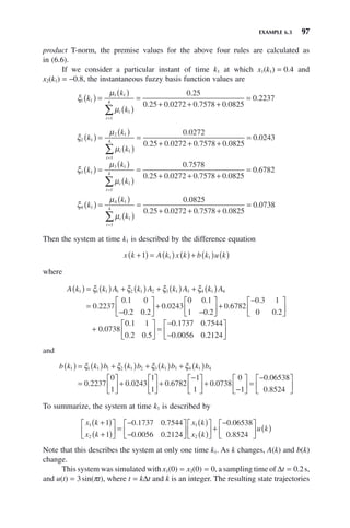
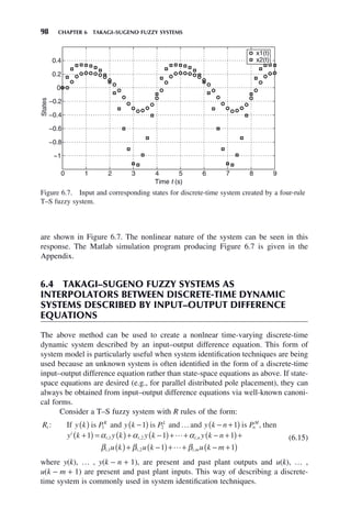
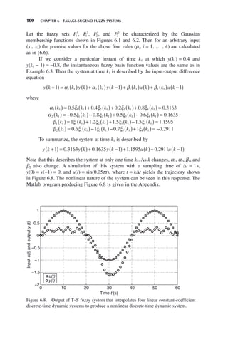
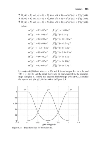
124. 106
Fuzzy Control and Identification, By John H. Lilly
Copyright © 2010 John Wiley Sons, Inc.
If a plant has a model in the form of a Takagi–Sugeno (T–S) fuzzy system that inter-
polates linear dynamic systems, which we call the plant fuzzy system, one approach
to stabilizing it is called parallel distributed control (PDC) [9,17,29]. The basic phi-
losophy of PDC is to create a controller fuzzy system with rule premises identical to
those of the plant fuzzy system. In the controller fuzzy system, each rule’s consequent
is a control law designed to control the linear system in the corresponding consequent
of the plant fuzzy system. The overall control law is thus a weighted average of the
individual control laws, just as the overall nonlinear system is a weighted average of
the linear systems in each consequent of the plant fuzzy system.
Parallel distributed control is important because it constitutes a method of
controlling nonlinear systems. Furthermore, as will be seen in Chapter 10, a nonlin-
ear system can sometimes be identified online as a T–S fuzzy system. If a parallel
distributed controller can then be designed based on this identification, a type of
real-time control known as adaptive control can be effected for nonlinear systems.
The control methods utilized in this book in parallel distributed control
schemes are the ones contained in Chapter 5, that is pole placement, tracking, and
model reference. Pole placement via parallel distributed control has the distinct
advantage that there exist mathematical tools to prove closed-loop stability, as dis-
cussed in Theorems 7.1 and 7.2. Such tools are lacking for control via Mamdani
fuzzy systems.
7.1 CONTINUOUS-TIME SYSTEMS
Let the plant fuzzy system rule base consist of R rules of the form:
R x t P x t P x t P
x t A
i
K L
n n
M
i
: ,
If is and is and and is then
1 1 2 2
( ) ( ) ( )
( ) =
i i
x t b u t
( )+ ( )
(7.1)
Then the system is given by the nonlinear/time-varying model given by (6.8) and
(6.9).
PARALLEL DISTRIBUTED
CONTROL WITH TAKAGI–
SUGENO FUZZY SYSTEMS
CHAPTER 7

125. EXAMPLE 7.1 107
The parallel distributed pole placement controller for this system is another
fuzzy system with R rules of the form:
R x t P x t P x t P
u t k
i
K L
n n
M
i
i
If is and is and and is then
1 1 2 2
( ) ( ) ( )
( ) = −
,
x t
( )
(7.2)
where the eigenvalues of Ai − biki are as desired in the left half-plane (see Section
5.3.1). The resulting control law is
u t k t x t
i i
i
R
( ) = − ( )
⎡
⎣
⎢
⎤
⎦
⎥ ( )
=
∑ ξ
1
(7.3)
where ξi(t) are the fuzzy basis functions defined in (6.4).
Not every PDC controller produces a stable closed-loop system, despite the
fact that each consequent system in the plant fuzzy system is stabilized by the control
law in the corresponding consequent of the controller fuzzy system. Nevertheless,
we have the following stability result for pole placement via parallel distributed
control.
THEOREM 7.1 (CONTINUOUS-TIME PARALLEL
DISTRIBUTED POLE PLACEMENT)
In the parallel distributed pole placement scheme described by (7.1)–(7.3), assume
each consequent system of the plant fuzzy system is controllable. Then, x = 0 is
globally asymptotically stable if there exists a positive definite symmetric matrix G
such that for all i = 1 , … , R and j = 1, … , R,
G A b k A b k G
i i j i i j
−
( )+ −
( )
T
0 (7.4)
where M 0 means that the matrix M is negative definite.
The proof follows directly from Lyapunov stability theory. Note that the
inequality (7.4) must be satisfied by one matrix G for all combinations of i and j.
The inequality (7.4) is called a continuous-time linear matrix inequality (LMI)
[29–31]. LMIs, such as (7.4), are difficult to solve by hand. Therefore, there are
various computational tools to solve them.
EXAMPLE 7.1
Consider a nonlinear two-state dynamic system described by the T–S fuzzy system
1. If x1 is P1
1
and x2 is P2
1
, then ẋ1
(t) = A1x(t) + b1u(t).
2. If x1 is P1
1
and x2 is P2
2
, then ẋ2
(t) = A2 x(t) + b2u(t).
3. If x1 is P1
2
and x2 is P2
1
, then ẋ3
(t) = A3 x(t) + b3u(t).
4. If x1 is P1
2
and x2 is P2
2
, then ẋ4
(t) = A4x(t) + b4u(t).

126. 108 CHAPTER 7 PARALLEL DISTRIBUTED CONTROL WITH TAKAGI–SUGENO FUZZY SYSTEMS
where
A b A b
1 1 2 2
0 1
2 2
0
1
0 1
3 2
0
1
=
−
⎡
⎣
⎢
⎤
⎦
⎥
= ⎡
⎣
⎢
⎤
⎦
⎥
=
−
⎡
⎣
⎢
⎤
⎦
⎥
= ⎡
⎣
⎢
⎤
⎦
⎥
, , ,
A b A b
3 3 4 4
0 1
2 1
0
1
0 1
3 1
0
1
=
−
⎡
⎣
⎢
⎤
⎦
⎥
= ⎡
⎣
⎢
⎤
⎦
⎥
=
−
⎡
⎣
⎢
⎤
⎦
⎥
= ⎡
⎣
⎢
⎤
⎦
⎥
, , ,
Notice that each consequent system is controllable and unstable. The eigen-
values of A1 are 1 ± j, those of A2 are 1 2
± j , those of A3 are 0.5 ± j1.32, and those
of A4 are 0.5 ± j1.66. Therefore, this T–S fuzzy system is nonlinear and unstable.
To stabilize it, we design a parallel distributed pole placement controller with state
feedback control laws to place the closed-loop eigenvalues of each system at −1 ± j.
The parallel distributed controller is given by
1. If x1(t) is P1
1
and x2(t) is P2
1
, then u1
(t) = −k1x(t).
2. If x1(t) is P1
1
and x2(t) is P2
2
, then u2
(t) = −k2x(t).
3. If x1(t) is P1
2
and x2(t) is P2
1
, then u3
(t) = −k3x(t).
4. If x1(t) is P1
2
and x2(t) is P2
2
, then u4
(t) = −k4x(t).
where k1 = [0 4], k2 = [−1 4], k3 = [0 3], and k4 = [−1 3]. Then the control
law applied to the plant is
u t k t k t k t k t x t
( ) = − ( )+ ( )+ ( )+ ( )
[ ] ( )
1 1 2 2 3 3 4 4
ξ ξ ξ ξ (7.5)
The requirement (7.4) for stability amounts to 16 inequalities for this particular
problem. These are
G A b k A b k G
1 1 1 1 1 1 0
−
( )+ −
( )
T
G A b k A b k G
1 1 2 1 1 2 0
−
( )+ −
( )
T
G A b k A b k G
1 1 3 1 1 3 0
−
( )+ −
( )
T
G A b k A b k G
1 1 4 1 1 4 0
−
( )+ −
( )
T
G A b k A b k G
2 2 1 2 2 1 0
−
( )+ −
( )
T
G A b k A b k G
2 2 2 2 2 2 0
−
( )+ −
( )
T
G A b k A b k G
2 2 3 2 2 3 0
−
( )+ −
( )
T
G A b k A b k G
2 2 4 2 2 4 0
−
( )+ −
( )
T
G A b k A b k G
3 3 1 3 3 1 0
−
( )+ −
( )
T
G A b k A b k G
3 3 2 3 3 2 0
−
( )+ −
( )
T
G A b k A b k G
3 3 3 3 3 3 0
−
( )+ −
( )
T
G A b k A b k G
3 3 4 3 3 4 0
−
( )+ −
( )
T
G A b k A b k G
4 4 1 4 4 1 0
−
( )+ −
( )
T
G A b k A b k G
4 4 2 4 4 2 0
−
( )+ −
( )
T
G A b k A b k G
4 4 3 4 4 3 0
−
( )+ −
( )
T
G A b k A b k G
4 4 4 4 4 4 0
−
( )+ −
( )
T

127. 7.2 DISCRETE-TIME SYSTEMS 109
As stated above, all 16 of these inequalities must be satisfied by one positive definite
symmetric matrix G.
It may be verified that the matrix
G =
⎡
⎣
⎢
⎤
⎦
⎥
1509 347
347 653
satisfies these 16 LMIs. This G was found with the aid of the Matlab LMI Control
Toolbox. Therefore, we are assured that the above parallel distributed controller
renders the point x = 0 globally asymptotically stable in the above closed-loop
system.
Let the fuzzy sets P1
1
, P1
2
, P2
1
, and P2
2
be characterized by the membership
functions shown in Figures 6.1 and 6.2. With initial conditions x1(0) = 1, x2(0) = −1,
and with no feedback, the state trajectories of Figure 7.1 result. The trajectories
increase unboundedly because the open-loop system is unstable. With the same
initial conditions and parallel distributed pole placement feedback control law (7.5),
the trajectories of Figure 7.2 result, indicating a stable closed-loop system. The
Matlab program producing Figures 7.1 and 7.2 is given in the Appendix.
Figure 7.1. State trajectories of open-loop continuous-time T–S plant.
0 1 2 3 4 5 6
−300
−250
−200
−150
−100
−50
0
50
100
Time t (s)
States
x
1
,
x
2
7.2 DISCRETE-TIME SYSTEMS
Let the plant fuzzy system rule base consist of R rules of the form:
R x k P x k P x k P
x k
i
K L
n n
M
i
: ,
If is and is and and is then
1 1 2 2
1
( ) ( ) ( )
+
( ) =
A x k b u k
i i
( )+ ( ) (7.6)
Then the system obeys the nonlinear/time-varying model given by (6.12)
and (6.13).

128. 110 CHAPTER 7 PARALLEL DISTRIBUTED CONTROL WITH TAKAGI–SUGENO FUZZY SYSTEMS
The parallel distributed pole-placement controller for this system is another
fuzzy system with R rules of the form:
R x k P x k P x k P
u k k
i
K L
n n
M
i
: ,
If is and is and and is then
1 1 2 2
( ) ( ) ( )
( ) = −
i
i x k
( )
(7.7)
where the eigenvalues of Ai − biki are as desired inside the unit circle (see Section
5.3.1). The resulting control law is
u k k k x k
i i
i
R
( ) = − ( )
⎡
⎣
⎢
⎤
⎦
⎥ ( )
=
∑ ξ
1
(7.8)
where ξi are the fuzzy basis functions defined in (6.14). The stability result for
discrete-time parallel distributed control is as follows.
THEOREM 7.2 (DISCRETE-TIME PARALLEL
DISTRIBUTED POLE PLACEMENT)
In the parallel distributed pole placement scheme described by (7.6)–(7.8), assume
each consequent system of the plant fuzzy system is controllable. Then x = 0 is
globally asymptotically stable if there exists a positive definite symmetric matrix G
such that for all i = 1, … , R and j = 1, … , R,
A b k G A b k G
i i j i i j
−
( ) −
( )−
T
0 (7.9)
The inequality (7.9) is called a discrete-time LMI.
Figure 7.2. State trajectories of continuous-time T–S plant with parallel distributed pole
placement.
0 1 2 3 4 5 6
−1
−0.8
−0.6
−0.4
−0.2
0
0.2
0.4
0.6
0.8
1
Time t (s)
States
x
1
,
x
2

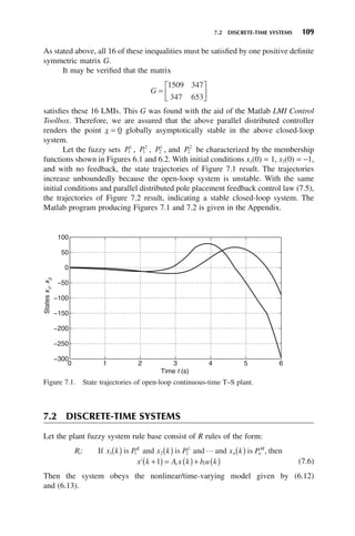
129. EXAMPLE 7.2 111
EXAMPLE 7.2
Consider a nonlinear dynamic system described by the T–S fuzzy system
1. If x1(k) is P1
1
and x2(k) is P2
1
, then x1
(k + 1) = A1x(k) + b1u(k).
2. If x1(k) is P1
1
and x2(k) is P2
2
, then x2
(k + 1) = A2 x(k) + b2u(k).
3. If x1(k) is P1
2
and x2(k) is P2
1
, then x3
(k + 1) = A3 x(k) + b3u(k).
4. If x1(k) is P1
2
and x2(k) is P2
2
, then x4
(k + 1) = A4x(k) + b4u(k).
where
A b A b
1 1 2 2
0 1
1 1
0
1
1 1
1 2
0
1
=
−
⎡
⎣
⎢
⎤
⎦
⎥ =
⎡
⎣
⎢
⎤
⎦
⎥ =
−
⎡
⎣
⎢
⎤
⎦
⎥ =
⎡
⎣
⎢
⎤
⎦
⎥
, , ,
A b A b
3 3 4 4
0 1
0 2 1
0
1
1 1
0 3 1
0
1
=
−
⎡
⎣
⎢
⎤
⎦
⎥ =
⎡
⎣
⎢
⎤
⎦
⎥ =
−
⎡
⎣
⎢
⎤
⎦
⎥ =
⎡
⎣
⎢
⎤
⎦
⎥
.
, ,
.
,
The eigenvalues of A1 are 0.5 ± j0.866, those of A2 are 1.5 ± j0.866, those of
A3 are 0.2764, 0.7236, and those of A4 are 1 ± j0.5477. Therefore, this T–S fuzzy
system is nonlinear and unstable, because the eigenvalues of A1, A2, and A4
have magnitudes that are not less than unity. To stabilize this system, we design a
parallel distributed controller with state feedback control laws to place the closed-
loop eigenvalues of each system at −0.5, 0.5. The parallel distributed controller is
given by
1. If x1(k) is P1
1
and x2(k) is P2
1
, then u1
(k) = −k1x(k).
2. If x1(k) is P1
1
and x2(k) is P2
2
, then u2
(k) = −k2x(k).
3. If x1(k) is P1
2
and x2(k) is P2
1
, then u3
(k) = −k3x(k).
4. If x1(k) is P1
2
and x2(k) is P2
2
, then u4
(k) = −k4x(k).
where
k k k k
1 2 3 4
1 25 1 0 25 3 0 45 1 0 45 2
= −
[ ] = −
[ ] = −
[ ] = [ ]
. , . , . , .
Then the control law applied to the system is
u k k k k k k k k k x k
( ) = − ( )+ ( )+ ( )+ ( )
[ ] ( )
1 1 2 2 3 3 4 4
ξ ξ ξ ξ (7.10)
Let the fuzzy sets P1
1
, P1
2
, P2
1
, and P2
2
be characterized by the membership
functions shown in Figures 6.1 and 6.2. With Δt = 0.1s, initial conditions x1(0) = 1,
x2(0) = −1, and with no feedback, the state trajectories of Figure 7.3 result.
The trajectories increase unboundedly because the open-loop system is unstable.
With the same initial conditions and parallel distributed pole placement feedback
control law (7.10), the trajectories of Figure 7.4 result, indicating a stable closed-
loop system. The Matlab program producing Figures 7.3 and 7.4 is given in the
Appendix.

130. 112 CHAPTER 7 PARALLEL DISTRIBUTED CONTROL WITH TAKAGI–SUGENO FUZZY SYSTEMS
7.3 PARALLEL DISTRIBUTED TRACKING CONTROL
The tracking control problem consists of determining a plant input such that the
plant output tracks a desired reference signal. A parallel distributed-type controller
can be designed to force the output of a nonlinear system modeled as a T–S fuzzy
system to track a desired reference signal. The controller design is explained in
Section 5.3.2 for a single linear plant. The parallel distributed tracking strategy is
to apply this design procedure to every consequent plant in the plant fuzzy system.
For tracking, the consequents in the plant fuzzy system are assumed to be in the
form of (5.11), that is, input–output difference equations.
Figure 7.4. State trajectories of discrete-time T–S plant with parallel distributed pole
placement.
0 0.1 0.2 0.3 0.4 0.5 0.6 0.7 0.8 0.9 1
−1
−0.8
−0.6
−0.4
−0.2
0
0.2
0.4
0.6
0.8
1
Time t
States
x
1
(t),
x
2
(t)
Figure 7.3. State trajectories of open-loop discrete-time T–S plant.
0 0.2 0.4 0.6 0.8 1 1.2 1.4 1.6 1.8 2
−10
−5
0
5
10
15
20
Time t
States
x
1
(t),
x
2
(t)
x1(t)
x2(t)

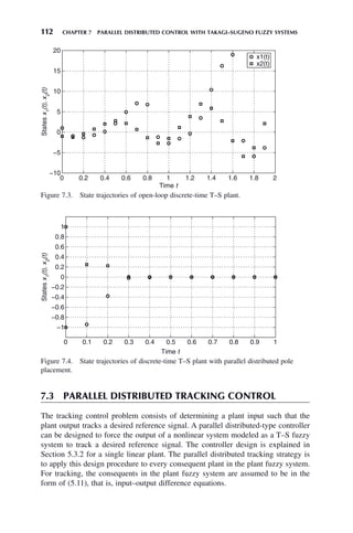
131. EXAMPLE 7.3 113
Let the plant fuzzy system rule base consist of R rules of the form:
R y k P y k P y k n P
y k
i
K L
n
M
i
: ,
If is and is and and is then
( ) −
( ) − +
( )
+
1 2
1 1
1
(
( ) = ( ) ( )+ ( ) ( )
− −
α β
i i
q y k q u k
1 1 (7.11)
where
αi i i i n
n
q a a q a q
− − − −
( )
( )= + + +
1
1 2
1 1
, , ,
(7.12a)
β β
i i i i m
m
i i
q b b q b q b q
− − − −
( )= + + + = + ′( )
1
0 1
1
0
1
, , , ,
(7.12b)
and q−1
is the backward shift operator defined by q−1
y(k) = y(k − 1).
The parallel distributed one-step-ahead tracking controller for this system is
another fuzzy system with R rules of the form:
R y k P y k P y k n P
u k
i
K L
n
M
i
: ,
If is and is and and is then
( ) −
( ) − +
( )
( )
1 2
1 1
= − ′( ) ( )+ +
( )− ( ) ( )
[ ]
− −
1
1
0
1 1
b
q u k r k q y k
i
i i
,
β α
(7.13)
The resulting control law is
u k u k k
i
i
i
R
( ) = ( ) ( )
=
∑ ξ
1
(7.14)
where ξi(k), i = 1, … , R are the fuzzy basis functions defined in (6.14). This design
procedure applies to n-step-ahead tracking problems with obvious modifications.
EXAMPLE 7.3
Consider the T–S fuzzy system with rule base:
1. If y(k) is P1
1
and y(k − 1) is P2
1
, then
y k y k y k u k u k
1
1 1 5 0 4 1 0 6 1
+
( ) = ( )− −
( )+ ( )+ −
( )
. . .
2. If y(k) is P1
1
and y(k − 1) is P2
2
, then
y k y k y k u k u k
2
1 0 4 1 8 1 1 2 1
+
( ) = ( )− −
( )+ ( )+ −
( )
. . .
3. If y(k) is P1
2
and y(k − 1) is P2
1
, then
y k y k y k u k u k
3
1 1 2 0 5 1 1 5 0 7 1
+
( ) = ( )+ −
( )+ ( )+ −
( )
. . . .
4. If y(k) is P1
2
and y(k − 1) is P2
2
, then
y k y k y k u k u k
4
1 0 8 1 6 1 1 5 1
+
( ) = ( )− −
( )+ ( )+ −
( )
. . .
The consequent systems are in the form of the consequent systems of (7.11) with
α α α
1
1 1
2
1 1
3
1 1
1 5 0 4 0 4 1 8 1 2 0 5
q q q q q q
− − − − − −
( )= − ( )= − ( )= +
. . , . . , . .
α β β
4
1 1
1
1 1
2
1 1
0 8 1 6 1 0 6 1 2
q q q q q q
− − − − − −
( )= − ( )= + ( )= +
. . , . , .

132. 114 CHAPTER 7 PARALLEL DISTRIBUTED CONTROL WITH TAKAGI–SUGENO FUZZY SYSTEMS
β β β
3
1 1
4
1 1
1 0 1
1 1
1 5 0 7 1 5 1 0 6
q q q q b q q
− − − − − −
( )= + ( )= + = ′( )=
. . , . , , . ,
, b
b2 0 1 2
, .
=
′( )= = ′( )= = ′( )
− − − − −
β β β
2
1 1
3 0 3
1 1
4 0 4
1
1 5 0 7 1 5
q q b q q b q
, . , . , . ,
, , and =
= −
q 1
Note that each consequent system is unstable because the polynomials
q q q q q q q q q q
2 1
1
1 2 2 1
2
1 2
1 1 5 0 4 1 0 4 1 8
− ( )
[ ]= − + − ( )
[ ]= − +
− − − −
α α
. . , . .
q q q q q q q q q q
2 1
3
1 2 2 1
4
1 2
1 1 2 0 5 1 0 8 1
− ( )
[ ]= − − − ( )
[ ]= − +
− − − −
α α
. . , .
and .
.6
each have roots outside the unit circle.
As an example, consider the third consequent plant above, that is,
y k y k y k u k u k
3
1 1 2 0 5 1 1 5 0 7 1
+
( ) = ( )+ −
( )+ ( )+ −
( )
. . . .
For this plant, we have α3(q−1
) = 1.2 + 0.5q−1
, β3(q−1
) = 1.5 + 0.7q−1
, b3,0 = 1.5, and
′( )=
− −
β3
1 1
0 7
q q
. . Therefore, (5.31) yields
1 5 0 7 1 1 2 0 5
1 3 1
. . . .
+
( ) ( ) = +
( )− +
( ) ( )
− −
q u k r k q y k
to give the tracking control law
u k u k y k y k r k
3 1
1 5
0 7 1 1 2 0 5 1 1
( ) = − −
( )− ( )− −
( )+ +
( )
[ ]
.
. . .
Using this design technique on all four consequent plants yields the parallel
distributed one-step-ahead tracking controller:
1. If y(k) is P1
1
and y(k − 1) is P2
1
, then
u k u k y k y k r k
1
0 6 1 1 5 0 4 1 1
( ) = − −
( )− ( )+ −
( )+ +
( )
. . .
2. If y(k) is P1
1
and y(k − 1) is P2
2
, then
u k u k y k y k r k
2 1
1 2
1 0 4 1 8 1 1
( ) = − −
( )− ( )+ −
( )+ +
( )
[ ]
.
. .
3. If y(k) is P1
2
and y(k − 1) is P2
1
, then
u k u k y k y k r k
3 1
1 5
0 7 1 1 2 0 5 1 1
( ) = − −
( )− ( )− −
( )+ +
( )
[ ]
.
. . .
4. If y(k) is P1
2
and y(k − 1) is P2
2
, then
u k u k y k y k r k
4 1
1 5
1 0 8 1 6 1 1
( ) = − −
( )− ( )+ −
( )+ +
( )
[ ]
.
. .
Let the input fuzzy sets P1
1
, P1
2
, P2
1
, and P2
2
be defined as in Figure 6.4. Let
the desired reference signal be r(k) = 0.5sin(0.2πk). With Δt = 1 second (hence
t = kΔt = k), initial conditions y(0) = 1, y(−1) = −1, a plot of y(t) together with r(t)
is shown in Figure 7.5 and the corresponding tracking error y(t) − r(t) is shown in
Figure 7.6.

133. EXAMPLE 7.3 115
The tracking is not perfect; for this example the tracking error always remains
in the range of ±10−3
because of the interpolation properties of the T–S fuzzy plant
and controller. The tracking would be perfect if each individual control law were
applied to each individual plant. This is not the case, however, with parallel
distributed-type controllers. Instead, we only have a weighted average of controllers
controlling a weighted average of plants. Therefore, the overall control is only an
approximation of the controller needed to effect perfect tracking for the overall plant,
which is in fact nonlinear.
The Matlab code that produced Figures 7.5 and 7.6 is given in the Appendix.
Figure 7.5. Tracking performance y(t) and r(t) of parallel distributed one-step-ahead
tracking controller.
0 2 4 6 8 10 12 14 16 18 20
−0.4
−0.2
0
0.2
0.4
0.6
0.8
1
Time t
Output
y(t)
r(t)
Figure 7.6. Tracking error y(t) − r(t) of parallel distributed one-step-ahead tracking
controller.
0 2 4 6 8 10 12 14 16 18 20
−0.2
0
0.2
0.4
0.6
0.8
1
Time t
Tracking
error
y(t)−r(t)

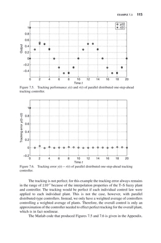
134. 116 CHAPTER 7 PARALLEL DISTRIBUTED CONTROL WITH TAKAGI–SUGENO FUZZY SYSTEMS
7.4 PARALLEL DISTRIBUTED MODEL
REFERENCE CONTROL
The model reference control problem consists of controlling the plant in such a way
that the controlled plant’s input–output behavior duplicates that of a desired refer-
ence model. A parallel distributed-type controller can be designed to control
a nonlinear plant modeled as a T–S fuzzy system to match a desired model. The
controller design is explained in Section 5.3.3 for a single linear plant. The parallel
distributed tracking strategy is to apply this design procedure to every consequent
plant in the plant fuzzy system. For model reference control, the consequents in the
plant fuzzy system are assumed to be in the form of (5.11) (i.e., input–output dif-
ference equations).
Let the plant fuzzy system rule base consist of R rules of the form (7.11) and
(7.12). Assume, without loss of generality, that the reference model is given by
(5.34). Then the parallel distributed model reference controller for this system is
another fuzzy system with R rules of the form:
R y k P y k P y k n P
u k
i
K L
n
M
i
: ,
If is and is and and is then
( ) −
( ) − +
( )
( )
1 2
1 1
= − ′( ) ( )− ( )−
( )+ ( )
[ ] ( )+ ( ) ( )
− − − −
1
1
0
1 1 1 1
b
q u k q E q q y k gH q r k
i
i i
,
β α
{ } (7.15)
The resulting control law is
u k u k k
i
i
i
R
( ) = ( ) ( )
=
∑ ξ
1
(7.16)
EXAMPLE 7.4
Consider the T–S fuzzy system of Example 7.3. Let the reference model have the
pulse transfer function
y k
r k
q q
q q
*( )
( )
=
+
+ +
− −
− −
2 0 6
1 0 5 0 5
1 2
1 2
.
. .
This can be expressed as (5.34) with g = 2, H(q−1
) = 1+ 0.3q−1
, and E(q−1
)
=1 + 0.5q−1
+ 0.5q−2
.
As an example, consider again the third consequent plant above, that is,
y k y k y k u k u k
3
1 1 2 0 5 1 1 5 0 7 1
+
( ) = ( )+ −
( )+ ( )+ −
( )
. . . .
For this plant, we have α3(q−1
) = 1.2 + 0.5q−1
, β3(q−1
) = 1.5 + 0.7q−1
, b3,0 = 1.5,
and ′( )=
− −
β3
1 1
0 7
q q
. . Therefore, (5.37) yields
γ q y k q u k q r k
− − −
( ) ( )+ +
( ) ( ) = +
( ) ( )
1 1 1
1 5 0 7 2 1 0 3
. . .
where γ(q−1
) is the unique polynomial of order 1 satisfying
1 0 5 0 5 1 1 2 0 5
1 2 1 1 1
+ + = + ( )− +
( )
[ ]
− − − − −
. . . .
q q q q q
γ

135. EXAMPLE 7.4 117
It is straightforward to show that γ(q−1
) = γ0 + γ1q−1
= 1.7 + q−1
. Therefore, (5.37)
yields the control law
u k u k y k y k r k r k
3 1
1 5
0 7 1 1 7 1 2 0 6 1
( ) = − −
( )− ( )− −
( )+ ( )+ −
( )
[ ]
.
. . .
Using the model reference control law (5.37) on each consequent plant yields
the parallel distributed model reference controller:
1. If y(k) is P1
1
and y(k − 1) is P2
1
, then
u k u k y k y k r k r k
1
0 6 1 2 0 1 1 2 0 6 1
( ) = − −
( )− ( )− −
( )+ ( )+ −
( )
. . .
2. If y(k) is P1
1
and y(k − 1) is P2
2
, then
u k u k y k y k r k r k
2 1
1 2
1 0 9 1 3 1 2 0 6 1
( ) = − −
( )− ( )+ −
( )+ ( )+ −
( )
[ ]
.
. . .
3. If y(k) is P1
2
and y(k − 1) is P2
1
, then
u k u k y k y k r k r k
3 1
1 5
0 7 1 1 7 1 2 0 6 1
( ) = − −
( )− ( )− −
( )+ ( )+ −
( )
[ ]
.
. . .
4. If y(k) is P1
2
and y(k − 1) is P2
2
, then
u k u k y k y k r k r k
4 1
1 5
1 1 3 1 1 1 2 0 6 1
( ) = − −
( )− ( )+ −
( )+ ( )+ −
( )
[ ]
.
. . .
Let the input fuzzy sets P1
1
, P1
2
, P2
1
, and P2
2
be defined as in Figure 6.4. Let
thedesiredreferencesignalber(k) = 0.5sin(0.2πk).WithΔt = 1s(hence,t = kΔt = k),
initial conditions y(0) = 1, y(−1) = −1, a plot of the output y(t) of the controlled plant
together with the model output ym(t) is shown in Figure 7.7 and the corresponding
error y(t) − ym(t) is shown in Figure 7.8.
Figure 7.7. Model matching performance y(t) and ym(t) of parallel distributed model
reference controller.
0 2 4 6 8 10 12 14 16 18 20
−0.8
−0.6
−0.4
−0.2
0
0.2
0.4
0.6
0.8
1
1.2
Time t
Output
y(t)
ym
(t)

136. 118 CHAPTER 7 PARALLEL DISTRIBUTED CONTROL WITH TAKAGI–SUGENO FUZZY SYSTEMS
The model following is not perfect; the absolute value of the error between
y(t) and ym(t) for this example always remains in the range of 0.025 because of the
interpolation properties of the T–S fuzzy plant and controller.
The Matlab code that produced Figures 7.7 and 7.8 is given in the
Appendix.
7.5 SUMMARY
As shown in Chapter 6, a T–S fuzzy system can be used to model a nonlinear
dynamic plant. We call this the plant fuzzy system. The rules of the plant
fuzzy system have consequents that are dynamic linear systems in continuous- or
discrete-time normal state space form, or linear input–output difference equation
form.
The parallel distributed control (PDC) strategy is to construct a controller
fuzzy system whose rule premises are identical to those of the plant fuzzy system,
and whose consequents are controllers designed for the corresponding plant in the
plant fuzzy system. If the plant fuzzy system consists of plants described by normal
form state equations, the controller fuzzy system’s consequents are linear state
feedback laws. This type of PDC results in nonlinear state regulation. Regulation
can be guaranteed if the feedback law satisfies a series of linear matrix inequalities
(LMI). Such guarantees are rare for closed-loop systems containing fuzzy control-
lers due to the complexity of fuzzy controllers.
If the plant fuzzy system consists of plants described by input–output differ-
ence equations, the controller fuzzy system consequents can be either tracking
control laws or model reference control laws. Remember that in the case of parallel
distributed output tracking or parallel distributed model reference control, there is
Figure 7.8. Model matching performance y(t) − ym(t) of parallel distributed model
reference controller.
0 2 4 6 8 10 12 14 16 18 20
−0.2
0
0.2
0.4
0.6
0.8
1
Time t
y(t)−y
m
(t)

137. EXERCISES 119
no formal proof that the control objective (i.e., output tracking or model following)
will be achieved. Nevertheless, these two approaches will be shown in Chapter 10
to be very useful for adaptive fuzzy control.
EXERCISES
7.1 Consider the system of Example 7.1. Design a parallel distributed controller
that places both closed-loop poles at −1.
7.2 Prove that the controller designed in Problem 7.1 stabilizes the closed-loop
system.
7.3 Simulate the closed-loop system designed in Problem 7.1. Use fourth-order
Runge–Kutta integration with a step size of 0.01s. Let x1(0) = 1, x2(0) = −1,
with fuzzy sets P1
and P2
specified by two triangular membership functions
with midpoints at x = −2, 2 such that they form a partition of unity.
7.4 Consider the system of Example 7.2. Design a parallel distributed controller
that places the closed-loop poles at 0.9 ± j0.1.
7.5 Prove that the controller designed in Problem 7.4 stabilizes the closed-loop
system.
7.6 Simulate the closed-loop system designed in Problem 7.4. Let x1(0) = 1,
x2(0) = −1, with fuzzy sets P1
and P2
specified by two triangular membership
functions with midpoints at x = −2, 2 such that they form a partition of
unity.
7.7 Consider the following T–S system:
1. If y(k) is P1
1
and y(k − 1) is P2
1
, then
y k y k y k u k u k
1
1 1 0 2 0 1 1
+
( ) = ( )− −
( )+ ( )+ −
( )
. .
2. If y(k) is P1
1
and y(k − 1) is P2
2
, then
y k y k y k u k u k
2
1 1 2 0 5 1 1 5 0 7 1
+
( ) = ( )+ −
( )+ ( )+ −
( )
. . . .
3. If y(k) is P1
2
and y(k − 1) is P2
1
, then
y k y k y k u k u k
3
1 0 4 1 8 1 1 2 1
+
( ) = ( )− −
( )+ ( )+ −
( )
. . .
4. If y(k) is P1
2
and y(k − 1) is P2
2
, then
y k y k y k u k u k
4
1 0 3 0 6 1 1 5 1
+
( ) = ( )− −
( )+ ( )+ −
( )
. . .
Design a parallel distributed tracking controller to make this system track the
reference signal r(k).
7.8 Simulate the closed-loop system designed in Problem 7.7. Let x1(0) = 1,
x2(0) = −1, with fuzzy sets P1
and P2
specified by two Gaussian membership
functions with midpoints at x = −2, 2 such that they cross at 0.4. Let
r(k) = 0.1(1 − cos(0.3k)). Plot y(k) − r(k), where y(k) is the output of the
controlled plant.

138. 120 CHAPTER 7 PARALLEL DISTRIBUTED CONTROL WITH TAKAGI–SUGENO FUZZY SYSTEMS
7.9 Consider the system of Problem 7.7. Design a parallel distributed model refer-
ence controller to make the controlled system’s model match the model
whose pulse transfer function is
G q
q q
q q
−
− −
− −
( )=
+
+ +
1
1 2
1 2
0 2
1 0 6 0 7
.
. .
7.10 Simulate the closed-loop system designed in Problem 7.9. Let x1(0) = 1,
x2(0) = −1, with fuzzy sets P1
and P2
specified by two triangular membership
functions with midpoints at x = −2, 2, such that they form a partition of unity.
Let the input to the reference model be r(k) = 0.1(1 − cos(0.3k)). Plot
y(k) − ym(k), where y(k) is the output of the controlled plant and ym(k) is the
output of the reference model.

139. 121
Fuzzy Control and Identification, By John H. Lilly
Copyright © 2010 John Wiley Sons, Inc.
In Chapters 3 and 6, we saw that some fuzzy systems have nonlinear memoryless
input–output characteristic functions. The nonlinear characteristic function of these
fuzzy systems is a result of the rules, T-norm, membership functions, and defuzzi-
fication method chosen by the designer. In these systems, the input and output
membership functions are fixed a priori.
It is also possible, given a particular nonlinear function, to find a fuzzy system
whose input–output characteristic matches it. In the fuzzy system, the output and in
some cases input membership functions are not fixed a priori, but are adjusted so
that the input–output characteristic most closely matches the nonlinear function in
some sense. The determination of a fuzzy system to approximate a given nonlinear
function is done utilizing well-known results from estimation theory. The estimation
methods introduced in this chapter are the least-squares and gradient approaches.
These are introduced because they have direct applications to control.
It will be seen in Chapter 9 that the ability to model static nonlinear functions
as fuzzy systems makes it possible to model dynamic nonlinear systems as fuzzy
systems. The motivation for modeling a dynamic nonlinear system as a fuzzy system
is that with such a model, the parallel distributed control methods of the previous
chapter can be employed to control the system. This enables a very powerful type
of control known as adaptive fuzzy control, introduced in Chapter 10. With adaptive
fuzzy control, tracking and model reference controllers can be designed for unknown
nonlinear systems.
8.1 LEAST-SQUARES ESTIMATION
The basic idea in least-squares estimation is to find parameters that minimize the
square of the difference between the estimated and true nonlinear functions. We first
introduce the batch least-squares approach, which finds the minimum based on a
finite number of stored input–output measurements from the plant. This process is
then made recursive resulting in an algorithm, called recursive least squares, that
updates the parameter estimate at each time step as new measurements are obtained
from the plant.
ESTIMATION OF STATIC
NONLINEAR FUNCTIONS
FROM DATA
CHAPTER 8

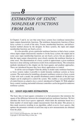
140. 122 CHAPTER 8 ESTIMATION OF STATIC NONLINEAR FUNCTIONS FOM DATA
8.1.1 Batch Least Squares [4,32]
Consider the algebraic system:
y j j j j
R R
( ) = ( ) + ( ) + + ( )
φ θ φ θ φ θ
1 1 2 2 (8.1)
where y(j), φi(j), i = 1, 2, … , R, j = 1, 2, 3, … are known and θ1, … , θR are unknown
constant parameters to be determined.
Defining the vectors
φ φ φ φ
j j j j R
R
T
( ) = ( ) ( ) ( )
[ ] ×
1 2 1
∼
θ θ θ θ
= [ ] ×
1 2 1
∼
R
T
R
the above system can be written as
y j j
T
( ) = ( )
φ θ (8.2)
This is called a regression model and φ(j) is called the regressor. Note that y(j) is
linear in the parameter vector θ.
Let k pairs of observations and corresponding regressors
y j j j k
( ) ( ) =
{ }
, , , , ,
φ 1 2
be obtained from k experiments performed on the system. This is sometimes called
training data. The objective is to estimate the unknown parameter vector θ from the
training data. The estimate will be called θ̂ .
To find the best θ̂, consider the performance measure
V y j j
T
j
k
1
2
1
1
2
ˆ ˆ
θ φ θ
( )= ( )− ( )
⎡
⎣ ⎤
⎦
=
∑ (8.3)
Then the best θ̂ , in a least-squares sense, is the one that minimizes V1 θ̂
( ). Defining
Y k y y y k k
T
( ) = ( ) ( ) ( )
[ ] ×
1 2 1
~
Φ k
k
k R
T
T
T
( ) =
( )
( )
( )
⎡
⎣
⎢
⎢
⎢
⎢
⎤
⎦
⎥
⎥
⎥
⎥
×
φ
φ
φ
1
2
~ (8.4)
then we can write the performance measure (8.3) as
V k Y k k k Y k k k
Y Y Y
T
T T
1
1
2
1
2
ˆ ˆ ˆ
ˆ
θ θ θ
θ
( )
( )= ( )− ( ) ( )
( ) ( )− ( ) ( )
( )
= − −
Φ Φ
Φ ˆ ˆ ˆ
ˆ ˆ ˆ
θ θ θ
θ θ θ
T T T T
T T T T T
Y
Y Y Y
Φ Φ Φ
Φ Φ Φ
+
( )
= − +
( )
1
2
2
(8.5)
where the dependence on k has been dropped for notational simplicity. The perfor-
mance measure V1 θ̂
( ) is quadratic and convex (i.e., bowl shaped with one unique
minimum) in parameter space. Therefore, to minimize V1 θ̂
( ) set

141. 8.1 LEAST-SQUARES ESTIMATION 123
∂ ( )
∂
=
V1
0
ˆ
ˆ
θ
θ
and solve for θ̂ :
∂ ( )
∂
= − + =
V
Y
T T
1
0
ˆ
ˆ
ˆ
θ
θ
θ
Φ Φ Φ
Therefore, θ̂ satisfying
Φ Φ Φ
T T
Y
θ̂ =
minimizes V1 θ̂
( ). If the matrix ΦT
Φ is invertible, the minimum is unique and is
given by
θ̂* k Y
T T
( ) = ( )−
Φ Φ Φ
1
(8.6)
This is the best least-squares estimate of θ based on the k measurements. It is
a batch calculation because we have to wait until k observations are made before
we can obtain θ̂*.
The fact that θ̂* is unique is a result of V1 θ̂
( ) in (8.5) being quadratic and
convex, which is a result of y in (8.2) being linear in the parameter estimates θ̂.
The requirement that ΦT
Φ be nonsingular is a persistent excitation requirement on
the regressor, which often consists of present and past values of the input or a com-
bination of the input and output or functions of these. Persistent excitation of the
regressor means that the regressor contains enough variation to permit accurate,
unique determination of θ̂*. It is always a requirement on the regressor frequency
content in all types of identification and estimation methods, fuzzy or not.
8.1.2 Recursive Least Squares
It is often desirable to make the estimation process recursive rather than batch. This
way, we would have an estimate θ̂ at every time step rather than having to wait k
time steps for one. When the batch least-squares estimation method is made recur-
sive, the parameter estimate at time k, θ̂ k
( ), is expressed in terms of the previous
estimate, θ̂ k −
( )
1 as follows.
Theorem: Let a single-output algebraic system be described by y(k) = φT
(x(k))θ,
where x(k) is the known system input at time k, y(k) is the known system output at
time k, φ(x(k)) ∼ R × 1 is a vector of known functions of the input, and θ ∼ R × 1
is an unknown vector of constants. Given initial conditions θ̂ k0
( ) and P(k0) ∼ R × R
symmetric positive definite, the recursive least-squares estimate θ̂ k
( ) satisfies:
ˆ ˆ ˆ
θ θ φ θ
k k K k y k k k
T
( ) = −
( )+ ( ) ( )− ( ) −
( )
⎡
⎣ ⎤
⎦
1 1 (8.7a)
K k P k k I k P k k
T
( ) = −
( ) ( ) + ( ) −
( ) ( )
[ ]−
1 1
1
φ φ φ (8.7b)
P k I K k k P k
T
( ) = − ( ) ( )
[ ] −
( )
φ 1 (8.7c)
Notice that for a single-output system, the bracketed term in (8.7b) is scalar.
Hence, in this case no matrix inversion is required, significantly reducing the com-
putational load. In (8.7a), the new parameter estimate θ̂ k
( ) is equal to the current

142. 124 CHAPTER 8 ESTIMATION OF STATIC NONLINEAR FUNCTIONS FOM DATA
one θ̂ k −
( )
1 plus a correction term that is a measure of how well the current esti-
mated system approximates the true process. In the term y k k k
T
( )− ( ) −
( )
⎡
⎣ ⎤
⎦
φ θ̂ 1 ,
y(k) is the output of the true process while φ θ
T
k k
( ) −
( )
ˆ 1 is the output of the current
estimated system.
Proof: This can be derived from the batch least-squares estimate (8.6) by writing
θ̂* k
( ) in terms of θ̂* k −
( )
1 , defining P(k) = [ΦT
(k)Φ(k)]−1
, and using the Matrix
Inversion Lemma: [A + BCD]−1
= A−1
− A−1
B(DA−1
B + C−1
)−1
DA−1
[33].
8.2 BATCH LEAST-SQUARES FUZZY ESTIMATION IN
MAMDANI FORM
Assume a fuzzy system with n inputs x = [x1, x2, … , xn], a single output y, and R
rules in the form
R x A x A x A y
i
K L
n n
M
: If is and is and and is , then
1 1 2 2 i
is Bi
(8.8)
Each rule has its own unique consequent fuzzy set Bi
characterized by a singleton
membership function located at y = bi
, i = 1, … , R, which is to be determined.
If the ith rule’s degree of firing (i.e., premise membership function) is μi(x),
the crisp output of the system is
f x
b x
x
b x b x b x
i
i
i
R
i
i
R
R
R
( ) =
( )
( )
= ( )+ ( )+ + ( )
=
=
∑
∑
μ
μ
ξ ξ ξ
1
1
1
1
2
2 (8.9)
where ξi(x) is the fuzzy basis function for the ith rule:
ξ
μ
μ
i
i
i
i
R
x
x
x
( ) =
( )
( )
=
∑
1
(8.10)
Since the input membership functions are fixed, the premise membership func-
tions μi(x) and the fuzzy basis functions ξi(x) are known a priori. Since the output
membership function locations bi
are unknown, the fuzzy system (8.9) is in the form
of (8.2), with φ ξ ξ ξ
T
R
x x x x
( ) = ( ) ( ) ( )
[ ]
1 2 and θ = [ ]
b b bR T
1 2
.
Therefore, batch or recursive least squares can be used to estimate the θ resulting in
the fuzzy system f(x) that best approximates a function g(x) in a least-squares sense.
EXAMPLE 8.1 (SINGLE INPUT FUNCTION)
Consider the function
g x x x x
( ) = − ( )+ ( )
cos . sin .
1 5 0 4 (8.11)

143. EXAMPLE 8.1 (SINGLE INPUT FUNCTION) 125
The output g is a nonlinear function of the input x. We wish to find a fuzzy system
f(x|θ) that approximates the nonlinear function g(x) over the interval 0 ≤ x ≤ 6.
Assume that we do this with a four-rule adjustable Mamdani fuzzy system. Let
the input fuzzy sets be characterized by Gaussian membership functions μi(x) =
exp(−0.5((x − ci
)/σi
)2
), i = 1, 2, 3, 4 with centers c1
= 0, c2
= 2, c3
= 4, c4
= 6
and spreads σ1
= σ2
= σ3
= σ4
= 1.184. The centers are chosen to cover the input
universe of discourse [0 6] evenly. The spreads are chosen so that adjacent mem-
berships cross at 0.7. The input memberships are shown in Figure 8.1.
Figure 8.1. Input membership functions for Example 8.1, σ = 1.184.
0 1 2 3 4 5 6
0
0.2
0.4
0.6
0.8
1
x
Membership
μ
μ1
μ2
μ3
μ4
Using product T-norm, the fuzzy basis functions are
ξ
σ
σ
j
j
j
i
i
x
x c
x c
( ) =
−
−
⎛
⎝
⎜
⎞
⎠
⎟
⎛
⎝
⎜
⎞
⎠
⎟
−
−
⎛
⎝
⎜
⎞
⎠
⎟
⎛
⎝
⎜
⎞
⎠
⎟
exp
exp
1
2
1
2
2
2
i
i=
∑
1
4
(8.12)
for j = 1, 2, 3, 4. These are plotted in Figure 8.2.
Since there are four rules, there are four unknown parameters (i.e., the output
centers b1
, … , b4
). We will estimate these with batch least squares. The input portion
of the training data should sufficiently cover the domain over which we desire a
good estimate of g. Since this domain is 0 ≤ x ≤ 6, let the input portion of the train-
ing data be the seven numbers x = [0 1 2 3 4 5 6]. The output portion
of the training data consists of the seven corresponding values of g, that is,
g = [−1 1.3187 3.7073 4.1428 4.0394 5.5627 7.5866]. Thus, the training
data in input–output pair form is
0 1 1 1 3187 2 3 7073 3 4 1428 4 4 0394 5 5 562
, , , . , , . , , . , , . , , .
−
( ) ( ) ( ) ( ) ( ) 7
7 6 7 5866
( ) ( )
{ }
, , .

144. 126 CHAPTER 8 ESTIMATION OF STATIC NONLINEAR FUNCTIONS FOM DATA
The crisp output of the fuzzy system is given by
y f x x x x x
b
b
b
b
x
T
= ( ) = ( ) ( ) ( ) ( )
[ ]
⎡
⎣
⎢
⎢
⎢
⎢
⎤
⎦
⎥
⎥
⎥
⎥
= ( )
θ ξ ξ ξ ξ φ θ
1 2 3 4
1
2
3
4
Then the batch least-squares estimate of θ is calculated as in (8.6) where
Y
T
= −
[ ]
1 1 3187 3 7073 4 1428 4 0394 5 5627 7 5866
. . . . . .
and
Φ =
( )
( ) ( )
( ) ( )
( ) ( )
( )
( )
( ) ( )
( ) ( )
( )
ξ ξ ξ ξ
ξ ξ ξ
1 2 3 4
1 2 3
1 1 1 1
2 2 2
x x x x
x x x ξ
ξ
ξ ξ ξ ξ
ξ ξ ξ
4
1 2 3 4
1 2
2
3 3 3 3
4 4
x
x x x x
x x
( )
( )
( )
( ) ( )
( ) ( )
( ) ( )
( )
( )
( ) ( )
( ) 3 4
1 2 3 4
1 2
4 4
5 5 5 5
6
x x
x x x x
x
( )
( ) ( )
( )
( )
( ) ( )
( ) ( )
( ) ( )
( )
( )
( )
ξ
ξ ξ ξ ξ
ξ ξ x x x
x x x x
6 6 6
7 7 7 7
3 4
1 2 3 4
( )
( ) ( )
( ) ( )
( )
( )
( ) ( )
( ) ( )
( ) ( )
( )
⎡
⎣
⎢
ξ ξ
ξ ξ ξ ξ
⎢
⎢
⎢
⎢
⎢
⎢
⎢
⎢
⎢
⎤
⎦
⎥
⎥
⎥
⎥
⎥
⎥
⎥
⎥
⎥
=
0 8042 0 1931 0 0027 0 0000
0 4859 0 4859 0
. . . .
. . .
. .
. . . .
. . . .
0280 0 0001
0 1618 0 6741 0 1618 0 0022
0 0273 0 4727 0 4727 0 027
73
0 0022 0 1618 0 6741 0 1618
0 0001 0 0280 0 4859 0 4859
0 0000 0
. . . .
. . . .
. .
. . .
0027 0 1931 0 8042
⎡
⎣
⎢
⎢
⎢
⎢
⎢
⎢
⎢
⎢
⎢
⎤
⎦
⎥
⎥
⎥
⎥
⎥
⎥
⎥
⎥
⎥
Figure 8.2. Fuzzy basis functions for Example 8.1, σ = 1.184.
−1 0 1 2 3 4 5 6 7
0
0.2
0.4
0.6
0.8
1
x
Basis
functions
ξ1
ξ2
ξ3
ξ4

145. EXAMPLE 8.1 (SINGLE INPUT FUNCTION) 127
Note that it is necessary to evaluate the fuzzy basis functions at the inputs of the
data set, that is, at x(1), x(2), … , x(7). Therefore, for example,
ξ2
2
4
1
2
3 2
1 184
0 4727
x( )
( ) =
−
−
⎛
⎝
⎜
⎞
⎠
⎟
⎛
⎝
⎜
⎞
⎠
⎟
=
exp
.
.
Δ
where
Δ = −
−
⎛
⎝
⎜
⎞
⎠
⎟
⎛
⎝
⎜
⎞
⎠
⎟ + −
−
⎛
⎝
⎜
⎞
⎠
⎟
⎛
⎝
⎜
⎞
⎠
⎟ +
exp
.
exp
.
1
2
3 0
1 184
1
2
3 2
1 184
2 2
e
exp
.
exp
.
−
−
⎛
⎝
⎜
⎞
⎠
⎟
⎛
⎝
⎜
⎞
⎠
⎟ + −
−
⎛
⎝
⎜
⎞
⎠
⎟
⎛
⎝
⎜
⎞
⎠
⎟
=
1
2
3 4
1 184
1
2
3 6
1 184
0
2 2
.
. . . .
0404 0 7 0 7 0 0404
+ + +
The batch LS algorithm (8.6) gives the following parameters:
ˆ
.
.
.
.
θ*=
b
b
b
b
1
2
3
4
2 6660
5 4934
2 6386
8 7027
⎡
⎣
⎢
⎢
⎢
⎢
⎤
⎦
⎥
⎥
⎥
⎥
=
−
⎡
⎣
⎢
⎢
⎢
⎢
⎤
⎦
⎥
⎥
⎥
⎥
⎥
This results in the fuzzy characteristic f x θ̂*
( ) shown in Figure 8.3. Even with so
few fuzzy sets and data points, the fit is still quite good.
Figure 8.3. Nonlinear function g(x) and its fuzzy approximation f x θ̂*
( ), σ = 1.184.
0 1 2 3 4 5 6
−2
−1
0
1
2
3
4
5
6
7
8
x
f(x)
g(x)
g(x)
f(x)
To see the effect of varying the spreads of the input membership functions,
let us keep the same centers with smaller spreads, that is, σ = 0.6444, which results
in adjacent Gaussians crossing at 0.3 (see Figs. 8.4 and 8.5).

146. 128 CHAPTER 8 ESTIMATION OF STATIC NONLINEAR FUNCTIONS FOM DATA
Figure 8.4. Input membership functions for Example 8.1, σ = 0.6444.
0 1 2 3 4 5 6
0
0.2
0.4
0.6
0.8
1
x
Membership
μ
μ1
μ2
μ3
μ4
Figure 8.5. Fuzzy basis functions for Example 8.1, σ = 0.6444.
−1 0 1 2 3 4 5 6 7
0
0.2
0.4
0.6
0.8
1
x
Basis
functions
ξ1
ξ2
ξ3
ξ4
When batch least squares is repeated with this σ, the following parameter vector
results:
ˆ
.
.
.
.
θ* =
⎡
⎣
⎢
⎢
⎢
⎢
⎤
⎦
⎥
⎥
⎥
⎥
=
−
⎡
⎣
⎢
⎢
⎢
⎢
⎤
⎦
b
b
b
b
1
2
3
4
1 0700
3 8262
4 0212
7 5119
⎥
⎥
⎥
⎥
⎥
The fuzzy characteristic is shown in Figure 8.6.

147. EXAMPLE 8.1 (SINGLE INPUT FUNCTION) 129
Figure 8.6. Nonlinear function g(x) and its fuzzy approximation f x θ̂*
( ), σ = 0.6444.
0 1 2 3 4 5 6
−2
−1
0
1
2
3
4
5
6
7
8
x
f(x)
g(x)
g(x)
f(x)
Figure 8.7. Input membership functions for Example 8.1, σ = 2.1784.
0 1 2 3 4 5 6
0
0.2
0.4
0.6
0.8
1
x
Membership
μ
μ1
μ2
μ3
μ4
The fit is not so good with σ = 0.6444. The input Gaussians (Fig. 8.4), and hence
the basis functions (Fig. 8.5), vary too quickly to accurately approximate the more
gently sloping function g(x).
If we try larger spreads, that is, σ = 2.1784, this results in adjacent Gaussians
crossing at 0.9 (see Figs. 8.7 and 8.8).

148. 130 CHAPTER 8 ESTIMATION OF STATIC NONLINEAR FUNCTIONS FOM DATA
Figure 8.8. Fuzzy basis functions for Example 8.1, σ = 2.1784.
−1 0 1 2 3 4 5 6 7
0
0.2
0.4
0.6
0.8
1
x
Basis
functions
ξ1
ξ2
ξ3
ξ4
Figure 8.9. Nonlinear function g(x) and its fuzzy approximation f x θ̂*
( ), σ = 2.1784.
0 1 2 3 4 5 6
−2
−1
0
1
2
3
4
5
6
7
8
x
f(x)
g(x)
g(x)
f(x)
When batch least squares is repeated with this σ, the following parameter vector
results:
ˆ
.
.
.
.
θ* =
⎡
⎣
⎢
⎢
⎢
⎢
⎤
⎦
⎥
⎥
⎥
⎥
=
−
−
⎡
⎣
⎢
b
b
b
b
1
2
3
4
18 0655
28 8548
18 9838
21 6675
⎢
⎢
⎢
⎢
⎤
⎦
⎥
⎥
⎥
⎥
The resulting fuzzy characteristic is shown in Figure 8.9.

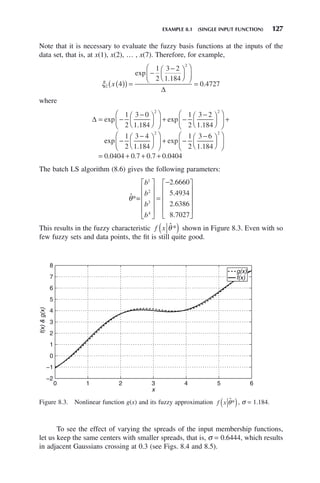
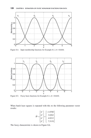
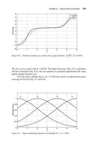
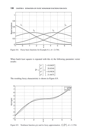
149. EXAMPLE 8.2 (MULTIPLE INPUT FUNCTION) 131
Again, the fit is not so good with σ = 2.1784. The input Gaussians (Fig. 8.7),
and hence the basis functions (Fig. 8.8), vary too slowly to accurately approximate
the more quickly changing function g(x).
This example illustrates the importance of choosing good input membership
functions when using least squares. The Matlab code producing the results for this
example is found in the Appendix .
EXAMPLE 8.2 (MULTIPLE INPUT FUNCTION)
Consider the function
g x x x x
1 2 1
2
2
, sin cos
( ) = (8.13)
The output g is a nonlinear function of the inputs x1 and x2, shown in Figure
8.10.
Figure 8.10. The function g(x1, x2) = sinx1cos2
x2.
−1 −0.5 0 0.5 1
−1
0
1
−1
−0.5
0
0.5
1
x
2
x1
g(x
1
,x
2
)
We wish to find a fuzzy system f((x1, x2)|θ) that approximates the nonlinear
function g(x1, x2) over the domain −1 ≤ x1 ≤ 1, −1 ≤ x2 ≤ 1. Let us do this with an
adjustable Mamdani fuzzy system with two inputs x1 and x2. On each universe, let
there be five Gaussian membership functions with centers [−1 −0.5 0 0.5 1]
and spreads σ = 0.2123 (so adjacent memberships cross at 0.5). For the rule
premises, use all possible combinations of these five fuzzy sets on both universes
resulting in 25 rules, each with its own adjustable consequent singleton fuzzy set
bi
, i = 1, 2, … , 25.
The fuzzy basis function for rule i is
ξ
μ
μ
i
i
j
j
x x
x x
x x
1 2
1 2
1 2
1
25
,
,
,
( ) =
( )
( )
=
∑

150. 132 CHAPTER 8 ESTIMATION OF STATIC NONLINEAR FUNCTIONS FOM DATA
where μi(x1, x2) is the premise value (i.e., degree of firing) of the ith rule.
The crisp output of this system is
f x x x x b
i
i
i
T
1 2 1 2
1
25
, ,
θ ξ φ θ
( ) = ( ) =
=
∑
The input portion of the training data should sufficiently cover the domain
over which we desire a good estimate of g. Since this domain is −1 ≤ x1 ≤ 1,
−1 ≤ x2 ≤ 1, let the input portion of the training data consist of 112
= 121 points
uniformly covering this domain, that is, all combinations of x1 = [−1, −0.8, −0.6,
… , 1], x2 = [−1, −0.8, −0.6, … , 1]. The output portion of the training data consists
of the 121 corresponding values of g(x1, x2) = sinx1cos2
x2.
The batch least-squares estimate of θ is calculated as in (8.6), where
ˆ ~
θ* 25 1
× , Φ ∼ 121 × 25, and Y ∼ 121 × 1. This results in a 2 input, 1 output fuzzy
system whose crisp output f(x1, x2) closely matches g(x1, x2). As a measure of the
closeness, the error surface |f(x1, x2) − g(x1, x2)| is shown in Figure 8.11. The
maximum distance between f(x1, x2|θ) and g(x1, x2) at the 121 data points is 0.0429,
indicating an excellent fit.
The Matlab program used for Example 8.2 is given in the Appendix .
Figure 8.11. Error surface |f − g| for Example 8.2.
−1
−0.5
0
0.5
1
−1
−0.5
0
0.5
1
0
0.01
0.02
0.03
0.04
0.05
x1
x
2
⏐f−g⏐
8.3 RECURSIVE LEAST-SQUARES FUZZY ESTIMATION
IN MAMDANI FORM
Assume a Mamdani fuzzy system with rules in the form of (8.8). The
resulting fuzzy system can again be described by (8.9), where the fuzzy
basis functions ξi(x) are fixed and known. Then the RLS algorithm proceeds
as in (8.7) with ˆ ˆ , ˆ , , ˆ
θ k b k b k b k
R
T
( ) = ( ) ( ) ( )
⎡
⎣ ⎤
⎦
1 2
… , y(k) = g(x(k)), and
φ ξ ξ ξ
T R
k x k x k x k
( ) = ( )
( ) ( )
( ) ( )
( )
[ ]
1 2
.

151. EXAMPLE 8.3 (SINGLE INPUT FUNCTION) 133
EXAMPLE 8.3 (SINGLE INPUT FUNCTION)
Consider again the system of Example 8.1 given by (8.11). This time, we will use
RLS to recursively find a fuzzy system f(x|θ) that approximates the nonlinear func-
tion g(x). Again, assume that we do this with an adjustable Mamdani fuzzy system
with four rules, four input fuzzy sets characterized by Gaussian membership func-
tions, and four adjustable output fuzzy sets characterized by singleton membership
functions. As above, we fix the input membership function centers and spreads. Then
the crisp output of the fuzzy system is given by (8.9).
Then, ˆ ˆ ˆ ˆ ˆ
θ k b k b k b k b k
( ) ( ) ( ) ( ) ( )
⎡
⎣ ⎤
⎦
1 2 3 4
would be recursively estimated as
in (8.7), where y(k) is the measured system output at time k (i.e., g(x(k))), and
φ ξ ξ ξ ξ
T
k x k x k x k x k
( ) = ( )
( ) ( )
( ) ( )
( ) ( )
( )
[ ]
1 2 3 4
is evaluated at each time k.
The time-varying fuzzy system is
f x k k
b k x k
x k
i
i
i
i
i
( ) ( )
( )=
( ) ( )
( )
( )
( )
=
=
∑
∑
ˆ
ˆ
θ
μ
μ
1
4
1
4
This fuzzy system changes for each k, but converges to the fuzzy system that
best approximates g(x) as k → ∞ in a least-squares sense given the chosen input
x(k).
The parameter estimates resulting from the RLS algorithm with x(k) = e(k), a
random variable uniformly distributed in [0 6] for each k, θ(0) = [0 0 0 0]T
,
and P(0) = 105
I are shown in Figure 8.12.
Figure 8.12. Parameter estimates from RLS algorithm.
0 20 40 60 80 100 120 140 160 180 200
−2
0
2
4
6
8
10
12
14
Time k
Parameter
Estimates
b1
b3
b2
b4

152. 134 CHAPTER 8 ESTIMATION OF STATIC NONLINEAR FUNCTIONS FOM DATA
Figure 8.13. Nonlinear function g(x) and its fuzzy approximation f(x|θ) with θ = [b1
, b2
,
b3
, b4
]* = [0.5314 9.0074 9.5993 12.6176].
0 1 2 3 4 5 6
−2
−1
0
1
2
3
4
5
6
7
8
x
f(x)
g(x)
g(x)
f(x)
The parameter estimates start at their initial conditions, transition through time, and
converge after ∼200 steps to the constant values [b1
(200) b2
(200) b3
(200) b4
(20
0)] = [0.5314 9.0074 9.5993 12.6176]. These final parameter values are not
unique, however. They depend on the input x(k), which is a random sequence.
Therefore, the final parameter values will be different every time the algorithm is run.
Figure 8.13 shows the fuzzy characteristic compared with g(x) for the above
parameter values. The fit is quite good; however it could be better if a more complex
fuzzy system (i.e., more rules) were used.
To summarize, the fuzzy system with the above characteristic that approxi-
mates g(x) is completely specified as follows:
Rule Base
1. If x is A1
, then f is b1
.
2. If x is A2
, then f is b2
.
3. If x is A3
, then f is b3
.
4. If x is A4
, then f is b4
.
where [b1
b2
b3
b4
]* = [0.5314 9.0074 9.5993 12.6176].
Input FuzzySets
μ1
2
1
2
1
1
x
x
( ) = −
−
⎛
⎝
⎜
⎞
⎠
⎟
⎡
⎣
⎢
⎤
⎦
⎥
exp
μ2
( ) = −
−
⎛
⎝
⎜
⎞
⎠
⎟
⎡
⎣
⎢
⎤
⎦
⎥
x
x
exp
.
1
2
2 5
1
2

153. 8.4 LEAST-SQUARES FUZZY ESTIMATION IN TAKAGI–SUGENO FORM 135
μ3
2
1
2
4
1
x
x
( ) = −
−
⎛
⎝
⎜
⎞
⎠
⎟
⎡
⎣
⎢
⎤
⎦
⎥
exp
μ4
2
1
2
5 5
1
x
x
( ) = −
−
⎛
⎝
⎜
⎞
⎠
⎟
⎡
⎣
⎢
⎤
⎦
⎥
exp
.
The premise values of the rules are the same as the input membership values because
there is only one input. Therefore, μi(x) = μi
(x). The input fuzzy sets are shown in
Fig. 8.14.
Figure 8.14. Input fuzzy sets (fixed).
−1 0 1 2 3 4 5 6 7
0
0.2
0.4
0.6
0.8
1
x
μ
A1
A2
A3
A4
Crisp Output
y x f x
b x
x
i
i
i
i
i
( ) = ( ) =
( )
( )
=
=
∑
∑
θ
μ
μ
1
4
1
4
In Figure 8.13, the fuzzy characteristic f is the one that results from using θ(200) in
the RLS algorithm.
8.4 LEAST-SQUARES FUZZY ESTIMATION IN
TAKAGI–SUGENO FORM
Assume a T–S fuzzy system with R rules in the form
R x A x A x A
q x a
i
K L
n n
M
i
: If is and is and is , then
1 1 2 2
( ) = 0 1 1 2 2
i i i
n
i
n
a x a x a x
+ + + +
(8.14)

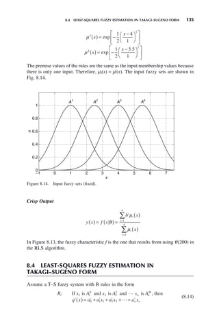
154. 136 CHAPTER 8 ESTIMATION OF STATIC NONLINEAR FUNCTIONS FOM DATA
The consequent qi
(x) is an affine function of the inputs x1, … , xn with the parameters
a a a a i R
i i i
n
i
0 1 2 1 2
, , , , , , , ,
… …
{ } = , unknown. If the premise membership function
for Rule i is μi(x), the output of the fuzzy system is
f x
q x
x
q x q x q x
a
i
i
i
R
i
i
R
R
R
( ) =
( )
( )
= ( )+ ( )+ + ( )
= +
=
=
∑
∑
μ
μ
ξ ξ ξ
1
1
1
1
2
2
0
1
a x a x a x x
a a x a x a x x
n n
n n
1
1
1 2
1
2
1
1
0
2
1
2
1 2
2
2
2
2
+ + +
[ ] ( )+
+ + + +
[ ] ( )
ξ
ξ + +
+ + + +
[ ] ( )
=
a a x a x a x x
R R R
n
R
n R
T
0 1 1 2 2 ξ
φ θ
where
φ ξ ξ ξ ξ ξ ξ ξ ξ ξ
T
R R n n n R
x x x x x x
= [ ]
1 2 1 1 1 2 1 1 2
(8.15a)
θ = [ ]
a a a a a a a a a
R R
n n n
R T
0
1
0
2
0 1
1
1
2
1
1 2
(8.15b)
The T–S fuzzy system is in the form of (8.2) with the unknown parameter
vector given by (8.15b) and the known regressor given by (8.15a). Thus the unknown
parameter vector θ can be estimated as above using either batch or recursive least
squares.
8.5 GRADIENT FUZZY ESTIMATION IN
MAMDANI FORM
It may be desirable to adjust input membership function centers and spreads as
well as output centers. This may be the case, for example, if we are unsure of
what the input fuzzy sets should be. If input memberships are to be adjusted, least-
squares methods cannot be used because it is no longer possible to express
the system as linear in the parameters. The gradient method [33,34] can be used to
adapt both input and output fuzzy sets (although other methods may be used as
well [35]).
The basic idea of the gradient method is to move the parameter estimate in a
direction that is opposite that of the gradient (or slope) of the error surface in param-
eter space. This insures the error always decreases with each new parameter update.
One problem with the gradient method is that the error surface is not convex so it
has many local minima. This means that the converged parameter vector depends
on the initial parameter guesses and may not be the one that produces the absolute
minimum error. Therefore, if the resulting fuzzy system does not approximate the
nonlinear function to sufficient accuracy, it may be beneficial to try different initial
parameter guesses.
Assume an n-input Mamdani fuzzy system with R rules, nR input fuzzy sets
characterized by Gaussian membership functions with adjustable centers cj
i
and

155. 8.5 GRADIENT FUZZY ESTIMATION IN MAMDANI FORM 137
spreads σ j
i
on each input universe (ith rule, jth universe of discourse), and R output
singleton fuzzy sets with adjustable locations bi
. Let the rule base of the system be
given by:
1 1 1
1
2 2
1 1
. ,
If is and is and and is then i
x A x A x A y
n n
s
s
If is and is and and is th
B
x A x A x A
n n
1
1 1
2
2 2
2 2
2
.
. ,
e
en is
R If is and is and and is
y B
x A x A x
R R
n
2
1 1 2 2
.
.
A y B
n
R R
, .
then is
(8.16)
Notice that these rules are in a slightly different form than we have been
considering in that each rule has its own unique premise and consequent fuzzy sets.
For instance, the fuzzy sets Aj
1
, j = 1, 2, … , n and B1
in (8.16) are used only for
the premise and consequent of Rule 1 and not for any other rule (see Fig. 8.15). This
is in contrast to rule bases seen previously in this book, in which a relatively small
number of fuzzy sets are defined on each input universe and a rule is written for
every possible combination of these.
Figure 8.15. Arrangement of inputs and rules corresponding to rule base (8.16). The
fuzzy sets are not necessarily in the order shown, that is, all of Rule 1’s fuzzy sets are not
necessarily leftmost.
Rule 1 Rule 2 Rule R
A1
1
A1
2
A1
R
A2
1
A2
2
A2
R
An
1
An
2
An
R

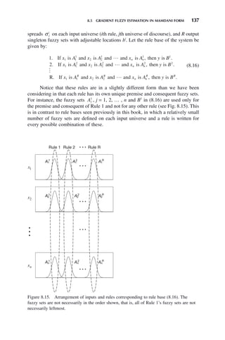
156. 138 CHAPTER 8 ESTIMATION OF STATIC NONLINEAR FUNCTIONS FOM DATA
Note also that the above form (8.16) for the rule base does not exclude rule
bases with rules in the form of (8.8) (e.g., the rule base of the fuzzy controller for
the ball and beam of Section 4.1.2). Rule bases with rules in the form of (8.8) tend
to be more intuitive for heuristic controller design than the form of (8.16). The form
seen in (8.8) can be used when the input fuzzy sets are fixed a priori and are not
adjusted in the estimation process, such as least-squares estimation methods. On the
other hand, rule bases of the form (8.16) must be used in methods where the input
memberships are adjusted, such as gradient-based algorithms.
For the rule base of (8.16), assuming we use Gaussian input membership
functions, the membership function characterizing Aj
i
(ith rule, jth universe) is
given by
μ
σ
j
i
j
j j
i
j
i
x
x c
( ) = −
−
⎛
⎝
⎜
⎞
⎠
⎟
⎛
⎝
⎜
⎞
⎠
⎟
exp
1
2
2
(8.17)
Note that this is a different notation from what we have previously used. In the
previous notation, the superscript denoted a particular fuzzy set on a universe [see
(3.2)]. In this new notation, the superscript denotes the rule number.
Using product T-norm, the premise value of Rule i of rule base (8.16) is
μ
σ
i n
j j
i
j
i
j
n
x x x
x c
1 2
2
1
1
2
, , , exp
( ) = −
−
⎛
⎝
⎜
⎞
⎠
⎟
⎛
⎝
⎜
⎞
⎠
⎟
=
∏ (8.18)
Then, the fuzzy system input–output characteristic is given by
f x
b
x c
x c
i j j
i
j
i
j
n
i
R
j j
i
θ
σ
( ) =
−
−
⎛
⎝
⎜
⎞
⎠
⎟
⎛
⎝
⎜
⎞
⎠
⎟
−
−
=
=
∏
∑ exp
exp
1
2
1
2
2
1
1
σ
σ
μ
μ
j
i
j
n
i
R
i
i
i
R
i
i
R
b x
x
⎛
⎝
⎜
⎞
⎠
⎟
⎛
⎝
⎜
⎞
⎠
⎟
=
( )
( )
=
=
=
=
∏
∑
∑
∑
2
1
1
1
1
(8.19)
Now assume we are given the kth training data pair (x(k), y(k)). Let the instan-
taneous estimation error corresponding to this pair be defined as
e k f x k y k
( ) = ( )
( )− ( )
[ ]
1
2
2
θ (8.20)
We seek to reduce e(k) by choice of parameters θ (i.e., bi
, cj
i
, σ j
i
). Use bi
(k),
c k
j
i
( ), σ j
i
k
( ) to denote these parameters’ values at time k. The basic gradient
method of parameter update is
b k b k
e k
b k
i i
i
+
( ) = ( )−
∂ ( )
∂ ( )
1 1
λ (8.21a)

157. 8.5 GRADIENT FUZZY ESTIMATION IN MAMDANI FORM 139
c k c k
e k
c k
j
i
j
i
j
i
+
( ) = ( )−
∂ ( )
∂ ( )
1 2
λ (8.21b)
σ σ λ
σ
j
i
j
i
j
i
k k
e k
k
+
( ) = ( )−
∂ ( )
∂ ( )
1 3 (8.21c)
Thus, the new value of a parameter equals the current value plus a correction in the
negative direction of the gradient of e(k) with respect to the parameter in parameter
space. The constants λ1, λ2, and λ3 are user-defined and determine the size of the
step taken in the direction of the negative gradient. In this way, it is insured that e(k)
decreases (or at worst does not increase) at every time step.
Note that in this book Gaussian membership functions are always used when
gradient parameter update is used, because it is much more straightforward to take
derivatives of Gaussians with respect to their parameters than it is to take derivatives
of triangulars with respect to theirs.
Calculating the gradients ∂e(k)/∂bi
(k), ∂ ( ) ∂ ( )
e k c k
j
i
, and ∂ ( ) ∂ ( )
e k k
j
i
σ is
done by applying the chain rule for differentiation. The process is similar to calcula-
tion of weight updates via backpropagation for neural networks. To find ∂e(k)/∂bi
(k),
we note from (8.20) that bi
is not mentioned explicitly in e(k), but only implicitly
through f. Therefore, we cannot directly calculate ∂e(k)/∂bi
(k), but instead must do
it implicitly using the chain rule of differentiation. Suppressing the time increment
k for notational simplicity, we have from (8.20):
∂
∂
=
∂
∂
∂
∂
e
b
e
f
f
b
i i
The partial ∂e/∂f can be obtained directly from (8.20) as
∂
∂
= − =
e
f
f y : ε (8.22)
The partial ∂f/∂bi
can be obtained from (8.9), which can be rewritten as
f b b b
j j
R R
j
= + + +
∑ ∑ ∑
1 1 2 2
μ
μ
μ
μ
μ
μ
(8.23)
Therefore, we have
∂
∂
=
=
∑
f
bi
i
j
j
R
μ
μ
1
(8.24)
giving the update law for bi
:
b k b k k
x k
x k
i i i
i
i
R
+
( ) = ( )− ( )
( )
( )
( )
( )
=
∑
1 1
1
λ ε
μ
μ
(8.25)
Similarly, for ∂ ( ) ∂
e k cj
i
we note from (8.20) that cj
i
is not mentioned explic-
itly in e(k) and not explicitly in f (8.23). However, it is an explicit factor in μi which

158. 140 CHAPTER 8 ESTIMATION OF STATIC NONLINEAR FUNCTIONS FOM DATA
is an explicit factor in f, which is an explicit factor in e(k). Therefore, we calculate
∂ ( ) ∂
e k cj
i
using the chain rule as
∂
∂
=
∂
∂
∂
∂
∂
∂
e
c
e
f
f
c
j
i
i
i
j
i
μ
μ
The partial ∂e/∂f is calculated in (8.22). The partial ∂f/∂μi is calculated from
(8.23) as
∂
∂
=
∂
∂
+ + +
+ + +
⎛
⎝
⎜
⎞
⎠
⎟ =
⎛
⎝
⎜
⎞
⎠
⎟
1
1
=
∑
f b b b
b
i i
R
R
R
j
j
R
i
μ μ
μ μ μ
μ μ μ
μ
1 2
2
2
1
−
−
⎛
⎝
⎜
⎞
⎠
⎟ ( )
⎛
⎝
⎜
⎞
⎠
⎟
=
−
=
=
=
∑
∑
∑
b
b f
j
j
j
R
j
j
R
i
j
j
R
μ
μ
μ
1
1
2
1
1
(8.26)
The partial ∂ ∂
μi j
i
c is calculated from (8.18), which can be rewritten as
μ σ σ σ
i
x c x c x c
x e e e
i
i
i
i
n n
i
( ) =
−
−
⎛
⎝
⎜
⎞
⎠
⎟ −
−
⎛
⎝
⎜
⎞
⎠
⎟ −
−
1
2
1
2
1
2
1 1
1
2
2 2
2
2
n
n
i
⎛
⎝
⎜
⎞
⎠
⎟
2
(8.27)
Then
∂
∂
=
⎧
⎨
⎪
⎩
⎪
⎫
⎬
⎪
⎭
⎪
−
−
⎛
⎝
⎜
⎞
⎠
⎟
=
− −
−
∏
μ σ σ
i
j
i
x c
k
j
x c
c
e e
k k
i
k
i
k k
i
k
i
1
2
2
1
2
1
1
⎛
⎛
⎝
⎜
⎞
⎠
⎟
= +
−
−
⎛
⎝
⎜
⎜
⎞
⎠
⎟
⎟
∏
⎧
⎨
⎪
⎩
⎪
⎫
⎬
⎪
⎭
⎪
−
−
⎛
2
1
2
2
1
k j
n
x c
j j
i
j
i
e
x c
j j
i
j
i
σ
σ
⎝
⎝
⎜
⎞
⎠
⎟
⎛
⎝
⎜
⎞
⎠
⎟ −
⎛
⎝
⎜
⎞
⎠
⎟
=
−
( )
1
2
σ
μ
σ
j
i
i
j j
i
j
i
x c
(8.28)
Combining these we obtain the update law for cj
i
:
c k c k k
b k f x k k
x k
j
i
j
i
i
i
i
R
+
( ) = ( )− ( )
( )− ( ) ( )
( )
( )
( )
⎡
⎣
⎢
⎢
⎢
⎢
=
∑
1 2
1
λ ε
θ
μ
⎤
⎤
⎦
⎥
⎥
⎥
⎥
( )
( )
( )− ( )
( )
( )
⎛
⎝
⎜
⎞
⎠
⎟
μ
σ
i
j j
i
j
i
x k
x k c k
k
2
(8.29)
For ∂ ( ) ∂
e k j
i
σ , we note from (8.20) that σ j
i
is not mentioned explicitly in
e(k) and not explicitly in f. However, it is an explicit factor in μi which is an explicit
factor in f, which is an explicit factor in e(k). Therefore, we calculate ∂ ( ) ∂
e k j
i
σ
using the chain rule as
∂
∂
=
∂
∂
∂
∂
∂
∂
e e
f
f
j
i
i
i
j
i
σ μ
μ
σ
The partials ∂e/∂f and ∂f/∂μi are the same as above (8.22) and (8.26). The partial
∂ ∂
μ σ
i j
i
is calculated similarly to ∂ ∂
μi j
i
c from (8.27) as follows:

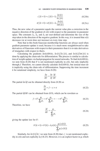
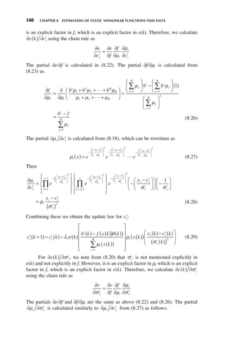
159. EXAMPLE 8.4 141
∂
∂
=
⎧
⎨
⎪
⎩
⎪
⎫
⎬
⎪
⎭
⎪
−
−
⎛
⎝
⎜
⎞
⎠
⎟
=
− −
−
∏
μ
σ
σ σ
i
j
i
x c
k
j
x c
e e
k k
i
k
i
k k
i
k
i
1
2
2
1
2
1
1
⎛
⎛
⎝
⎜
⎞
⎠
⎟
= +
−
−
⎛
⎝
⎜
⎜
⎞
⎠
⎟
⎟
∏
⎧
⎨
⎪
⎩
⎪
⎫
⎬
⎪
⎭
⎪
−
−
⎛
2
1
2
2
1
k j
n
x c
j j
i
j
i
e
x c
j j
i
j
i
σ
σ
⎝
⎝
⎜
⎞
⎠
⎟
⎛
⎝
⎜
⎞
⎠
⎟ −
−
( )
⎛
⎝
⎜
⎞
⎠
⎟
=
−
( )
( )
x c
x c
j j
i
j
i
i
j j
i
j
i
σ
μ
σ
2
2
3
By combining these, we obtain the update law for σ j
i
as
σ σ λ ε
θ
μ
j
i
j
i
i
i
i
R
k k k
b k f x k k
x k
+
( ) = ( )− ( )
( )− ( ) ( )
( )
( )
( )
⎛
⎝
⎜
⎜
⎜
⎜
=
∑
1 3
1
⎞
⎞
⎠
⎟
⎟
⎟
⎟
( )
( )
( )− ( )
( )
( )
( )
μ
σ
i
j j
i
j
i
x k
x k c k
k
2
3
(8.30)
Equations (8.25), (8.29) and (8.30) give the update laws for the parameters bi
, cj
i
,
and σ j
i
of the fuzzy system.
In these update laws, the magnitude of the correction is proportional to the
constant λi, which is user-selected. If λi is small, the rate of convergence is slow,
and if λi is large, the rate of convergence is fast. Note, however, that if λi is too
small, convergence may take too long. If λi is too large, convergence may not occur
at all because each update step in the vicinity of the local minimum is too large to
find the minimum.
The gradients in the update laws depend on the training data pairs (x(k), y(k))
taken from the system. If several pairs of training data are available, which is
usually the case, the above algorithm could be run over and over for the first pair
of data until convergence occurs, then iterate again using the second pair of data
with the converged parameters of the first set as initial conditions, and so on.
Alternatively, we could run through the entire set of training data once for each
pair, then iterate over the entire set repeatedly until convergence is obtained. The
latter method is used in this text for test data consisting of a finite number of pairs.
In adaptive identifiers and controllers, the new data is fed to the algorithm as it
occurs.
EXAMPLE 8.4
Consider again the function (8.11). Let 200 data pairs be taken, that is, {(x(1), y(1)),
(x(2), y(2)), … , (x(200), y(200))}, where x(k) is a random variable uniformly dis-
tributed in [0 6] for each k. Let there be five rules and five Gaussian input fuzzy
sets, one for each rule. Therefore, we have 15 parameters to adjust: five input centers,
five input spreads, and five output singleton locations. The initial parameter values
are chosen randomly within the range of the training data. Since the input ranges
between 0 and 6, we choose five values randomly in this range for initial values of
ci
, i = 1, … , 5. Similarly, we choose five values randomly in [0 15] for initial
values of bi
, i = 1, … , 5. The initial values of σi
, i = 1, … , 5, are randomly chosen

160. 142 CHAPTER 8 ESTIMATION OF STATIC NONLINEAR FUNCTIONS FOM DATA
Figure 8.17. Estimates of output membership function centers.
0 50 100 150 200 250 300 350 400
0
2
4
6
8
10
12
Training step k
Parameter
estimates
b1
b2
b3
b4
b5
from [0 2]. Note that if we have some idea of the correct parameter values, we
should use these as initial conditions for the gradient algorithm. The step sizes are
chosen as λ1 = λ2 = λ3 = 0.001.
The characteristic of the converged fuzzy system after 400 training steps (i.e.,
twice through the training data) is shown in Figure 8.16. The fit is not good after so
few training steps. The evolution of the parameter estimates is shown in Figures
8.17–8.19. From these figures, it is evident that convergence has not occurred after
400 training steps.
Figure 8.16. Comparison of f and g, twice through training data.
0 1 2 3 4 5 6
−1
0
1
2
3
4
5
6
7
8
x
f(x)
g(x)
g(x)
f(x)

161. EXAMPLE 8.4 143
Figure 8.18. Estimates of input membership function centers.
0 50 100 150 200 250 300 350 400
0
1
2
3
4
5
6
7
8
Training Step
Parameter
Estimates
c1
c2
c3
c4
c5
Figure 8.19. Estimates of input membership function spreads.
0 50 100 150 200 250 300 350 400
−2
−1.5
−1
−0.5
0
0.5
1
1.5
2
Training step k
Parameter
Estimates
σ1
σ2
σ4
σ3
σ5
If we perform 105
training steps (i.e., 500 times through the training data), the
estimates have converged and the fuzzy characteristic f(x) is indistinguishable from
g(x), that is, the approximation is excellent.
After 105
training steps, the input centers and spreads have converged to
c* = [5.8952 2.4475 4.0362 2.2839 1.0931] and σ* = [1.4974 0.7503
0.8877 1.1236 2.0125], producing the input memberships shown in Figure
8.20.

162. 144 CHAPTER 8 ESTIMATION OF STATIC NONLINEAR FUNCTIONS FOM DATA
Figure 8.21. Output membership functions determined by gradient method.
−2 0 2 4 6 8
0
0.2
0.4
0.6
0.8
1
x
Membership
μ
b2
b4
b3
b1
b5
The output singleton locations have converged to b* = [8.4704 6.9878
3.2109 6.1789 −2.1289], producing the output memberships shown in Figure
8.21.
Figure 8.20. Input membership functions determined by gradient method.
0 1 2 3 4 5 6
0
0.2
0.4
0.6
0.8
1
x
Membership
μ
μ5
μ4 μ3
μ2
μ1
Thus, the rule base of the fuzzy system approximating g(x) in (8.11) is
1. If x is A1
, then f is b1
.
2. If x is A2
, then f is b2
.
3. If x is A3
, then f is b3
.
4. If x is A4
, then f is b4
.
5. If x is A5
, then f is b5
.

163. 8.6 GRADIENT FUZZY ESTIMATION IN TAKAGI–SUGENO FORM 145
Note that for each different set of initial conditions and training data, the gradient
algorithm produces a different fuzzy system, that is, different input and output
memberships. This is due to the fact that the error function for the gradient method
does not have one unique minimum, but rather many local minima. For most reason-
able initial parameter guesses and training data, the gradient algorithm will eventu-
ally converge to a fuzzy system whose input–output characteristic closely matches
g(x). Each fuzzy system is different, depending on the initial parameter guesses and
training data used. A good fit to g(x) is not guaranteed, however.
8.6 GRADIENT FUZZY ESTIMATION IN
TAKAGI–SUGENO FORM
Assume an n-input T–S fuzzy system with R rules, nR input fuzzy sets characterized
by Gaussian membership functions with adjustable centers cj
i
and spreads σ j
i
on
each input universe (ith rule, jth universe of discourse), and R consequents consisting
of affine functions with n + 1 adjustable parameters aj
i
. Let the rule base be given
by
1 1 1
1
2 2
1 1
1
. If is and is and and is , then
x A x A x A
q x
n n
( )
) = + + +
a a x a x a x
x A x A
n n
0
1
1
1
1 2
1
2
1
1 1
2
2 2
2
2
. If is and is and
and is , then
R If
x A
q x a a x a x a x
x
n n
n n
2
2
0
2
1
2
1 2
2
2
2
1
( ) = + + +
. is and is and and is , then
A x A x A
q x a
R R
n n
R
R R
1 2 2
0
( ) = + a x a x a x
R R
n
R
n
1 1 2 2
+ +
(8.31)
The crisp output of this system is given by
f x
q x x
x
i
i
j
R
i
j
R
( ) =
( ) ( )
( )
=
=
∑
∑
μ
μ
1
1
where μi(x) are the premise membership functions defined in (8.18).
Now the parameters of the system are cj
i
, σ j
i
, and aj
i
. These are to be adjusted
using the gradient method. The adjustment of cj
i
and σ j
i
are the same and before
[(8.29) and (8.30)]. The update law for aj
i
is
a k a k
e k
a k
j
i
j
i
j
i
+
( ) = ( )−
∂ ( )
∂ ( )
1 4
λ (8.32)
The partial ∂ ( ) ∂
e k aj
i
is calculated using the chain rule for differentiation as above.
We note from (8.20) that aj
i
is not mentioned explicitly in e(k), but only implicitly
through f. Therefore, we cannot directly calculate ∂ ( ) ∂
e k aj
i
, but instead must do it
implicitly using the chain rule of differentiation:

164. 146 CHAPTER 8 ESTIMATION OF STATIC NONLINEAR FUNCTIONS FOM DATA
∂
∂
=
∂
∂
∂
∂
∂
∂
e
a
e
f
f
q
q
a
j
i i
i
j
i
The partial ∂e/∂f was calculated in (8.22). The partial ∂f/∂qi
can be obtained from
(8.23), which can be rewritten as
f q q q
j j
R R
j
= + + +
∑ ∑ ∑
2
1 1 2
μ
μ
μ
μ
μ
μ
This yields
∂
∂
=
∑
f
qi
i
i
μ
μ
The partial ∂ ∂
q a
i
j
i
depends on j, that is,
∂ ( )
∂
=
=
=
⎧
⎨
⎩
q x
a
j
x j n
i
j
i
j
1 0
1
,
, , ,
(8.33)
Therefore, the parameter update law for aj
i
is
a k a k k
x k
x k
q x k k
a
j
i
j
i i
i
j
R
i
j
i
+
( ) = ( )− ( )
( )
( )
( )
( )
∂ ( )
( )
∂
=
∑
1 4
1
λ ε
μ
μ
,
k
k
( ) (8.34)
with ∂ ∂
q a
i
j
i
as in (8.33). Then, the parameter update laws for T–S fuzzy systems
with affine consequents are given by (8.29), (8.30), and (8.34).
8.7 SUMMARY
This chapter explores the ability of fuzzy systems to estimate static functions. To
do this, input–output data must be available from the function. Although there are
many methods that can be used to create fuzzy systems that aproximate functions,
we concentrate on two: least squares and gradient. This is because these methods
are recursive, hence can be used for adaptive fuzzy control (Chapter 10).
In the case of least-squares estimation (whether batch or recursive), the fuzzy
system must be linear in the unknown parameters. Therefore, the input membership
functions must be fixed a priori and only the output parameters adjusted. Because
the error function is quadratic, it has a unique minimum in parameter space.
Therefore, the parameter estimates converge to unique values regardless of the initial
guess.
The recursive least-squares algorithm converges more quickly than some other
methods, specifically the gradient algorithm. Because least squares is limited to
adjusting only the output fuzzy sets, it is less flexible in constructing fuzzy systems
to estimate nonlinear functions than methods that adjust both input and output fuzzy
sets, specifically the gradient algorithm.

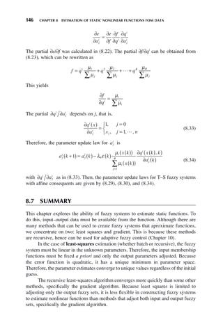
165. EXERCISES 147
If least squares is used, it is possible to use rules of the form found in Section
3.6 (wind chill system). This enables one to define intuitively a relatively small
number of fuzzy sets on each input universe and write rules whose premises are
various combinations of these. This produces a rule base that is transparent to human
understanding.
In the case of gradient adaptation, there is no requirement for the fuzzy system
to be linear in the parameters, so all input and output fuzzy sets can adjusted.
Because of this, each rule must have its own separate input fuzzy sets that are not
shared with any other rules. This necessitates a premise fuzzy set arrangement as in
(8.16) rather than that found in Section 3.6. Thus gradient-adapted rules are not as
easily understood as least-squares-adapted rules.
Gradient estimation takes longer to converge and may not converge at all in
a finite time interval. However, gradient estimation tends to be more flexible in its
estimation capabilities, due to the fact that the input memberships are adapted along
with the output parameters.
EXERCISES
8.1 In a generalization of the least squares algorithm presented in Section 8.1.1,
some data is weighted heavier than other data giving rise to the performance
measure
V w y j j
j
T
j
k
2
2
1
1
2
ˆ ˆ
θ φ θ
( )= ( )− ( )
⎡
⎣ ⎤
⎦
=
∑
where wj 0, j = 1, … , k. Derive the value of θ̂* that minimizes V2 (this is
called a weighted least-squares estimate).
8.2 Repeat Example 8.1 with 5 input fuzzy sets centered at [0 1.5 3 4.5
6]. Choose σ so the adjacent input membership functions cross at 0.5.
8.3 Derive the recursive least-squares algorithm (8.7) from the batch least-squares
estimate (8.6) by writing θ̂* k
( ) in terms of θ̂* k −
( )
1 , defining
P(k) = [ΦT
(k)Φ(k)]−1
, and using the Matrix Inversion Lemma.
8.4 Repeat Example 8.2 using data taken at points (x1, x2) = {(−1 −1), (−1, 0),
(−1, 1), (0, −1), (0, 0), (0, 1), (1, −1), (1, 0), (1, 1)}
8.5 Use RLS to find a two-rule T–S fuzzy system to approximate (8.11) on the
intertval 0 ≤ x ≤ 6. Let the rules be
1. If x is A1
, then q x a a x
1
0
1
1
1
( ) = + .
2. If x is A2
, then q x a a x
2
0
2
1
2
( ) = + .
Use triangular membership functions forming a partition of unity on the x
universe.
8.6 You are using RLS to find a four-rule T–S fuzzy system to approximate (8.13)
on the intertval −1 ≤ x1 ≤ 1, −1 ≤ x2 ≤ 1, as in Section 8.4. (a) Specify all
rules of the approximating fuzzy system. (b) Specify all fuzzy sets. (c) Specify

166. 148 CHAPTER 8 ESTIMATION OF STATIC NONLINEAR FUNCTIONS FOM DATA
the T-norm and method of defuzzification. (d) Specify the training data and
test data.
8.7 (a) Why are rules of the form found in Sect. 3.6 more desirable than rules of
the form (8.16)? (b) Why can rules like those in Sect. 3.6 not be used in
gadient-adjusted fuzzy systems if input membership functions are to be
adjusted?
8.8 Redo Example 8.3 with 3 Gaussian input fuzzy sets with centers at x = [0, 3,
6] such that adjacent memberships cross at 0.5.
8.9 Redo problem 8.8 with 3 triangular memberships located at x = [0, 3, 6] and
forming a partition of unity.
8.10 Assume a fuzzy system with rules of the form
R x A q x a x a x
i
i i i i
: sin cos
If is , then ( ) = ( )+ ( )
0 1
is to be adjusted via gradient. Write the gradient update equations for ai
0
and ai
1 .

167. 149
Fuzzy Control and Identification, By John H. Lilly
Copyright © 2010 John Wiley Sons, Inc.
The estimation methods of Chapter 8 can be used to find fuzzy models for nonlinear
dynamic systems. The determination of a model for an unknown system is known
as identification. Usually, the object of doing so is to utilize the model in a parallel
distributed control scheme (see Chapter 7). Design of a parallel distributed controller
is relatively straightforward because the consequents in the fuzzy model are linear
systems.
In Section 9.1, we present a method of deriving a fuzzy model for a nonlinear
system whose equations of motion are known. This enables parallel distributed
control of the nonlinear system when derivation of the controller directly from the
nonlinear equations of motion may he impossible.
If the controller is to be capable of adjusting itself in real time (as in adaptive
fuzzy control), the method used for identification must be recursive. In Chapter 8,
we give two methods of recursive identification: recursive least squares (RLS) and
gradient. Therefore, we will concentrate on these methods in this chapter.
9.1 MODELING KNOWN PLANTS AS
T–S FUZZY SYSTEMS [29]
Many nonlinear systems with known mathematical models may be exactly modeled
on a bounded domain in the state space with Takagi–Sugeno (T–S) fuzzy systems.
Consider a nonlinear time-invariant system for which x = 0 is the equilibrium point.
The basic idea of modeling it with a T–S fuzzy system is to express it as a series of
linear dynamic systems, each one the consequent of one of the rules. Functions zi
are determined such that nonlinear terms in the plant model can be expressed as zi x,
where x is a plant state. Each of these functions zi becomes an input to the fuzzy
system. Two fuzzy sets forming a partition of unity are defined on each zi universe,
centered at the maximum and minimum of zi.
Assume a scalar nonlinear function z(x) . If z(x) is to be modeled in the domain
X, let b z
m = ( )
min
X
and b z
M = ( )
max
X
. Then, create two fuzzy sets P1
and P2
on X
characterized by triangular membership functions μ1
(z) and μ2
(z) as
μ1
z
b z
b b
M
M m
( ) =
−
−
(9.1a)
MODELING OF DYNAMIC
PLANTS AS FUZZY SYSTEMS
CHAPTER 9

168. 150 CHAPTER 9 MODELING OF DYNAMIC PLANTS AS FUZZY SYSTEMS
μ2
z
z b
b b
m
M m
( ) =
−
−
(9.1b)
Then, z can be exactly represented on X as
z z b z b
m M
= ( ) + ( )
μ μ
1 2
(9.2)
This technique can be used to exactly model a nonlinear dynamic system as a
weighted average of linear systems.
EXAMPLE 9.1
Consider the nonlinear system ẋ = f(x) and assume that f(x) can be factored as z(x)x
[e.g., x3
can be factored as (x2
)x so that z(x) = x2
]. Now the nonlinear system can be
expressed as ẋ = z(x)x. In order to exactly model the system on the bounded domain
X as a T–S fuzzy system, let b z
m = ( )
min
X
and b z
M = ( )
max
X
.
Create two fuzzy sets MIN and MAX on X characterized by triangular mem-
bership functions μMIN
(z) and μMAX
(z), as in (9.1). These are shown in Figure 9.1.
Then the nonlinear system is exactly modeled on X by the T–S fuzzy system:
1. If z is MIN, then ẋ1
= bm x.
2. If z is MAX, then ẋ2
= bM x.
Figure 9.1. Fuzzy sets on z universe.
0
0.2
0.4
0.6
0.8
1
z
Membership
μ
MIN MAX
bM
bm
EXAMPLE 9.2
A nonlinear system has the mathematical model:
x x x
1 1 2
= (9.3a)
x x x x u
2 1 2
3 2
1
1
= − + +
( )
cos (9.3b)

169. EXAMPLE 9.2 151
It can be verified that this system is open-loop unstable [21,22]. Define z1 = x1,
z x
2 2
2
= , and z3 = 1 + cos2
x1. Then, (9.3) can be rewritten as
x
x
z
z
x
x z
u
1
2
1
2
1
2 3
0
1
0
⎡
⎣
⎢
⎤
⎦
⎥ =
−
⎡
⎣
⎢
⎤
⎦
⎥
⎡
⎣
⎢
⎤
⎦
⎥ +
⎡
⎣
⎢
⎤
⎦
⎥
We wish to derive a T–S fuzzy system whose behavior exactly duplicates
(9.3). Assume the bounded domain X is defined by x1 ∈ [−2, 2] and x2 ∈ [−2, 2]
[i.e., the T–S fuzzy system will duplicate (9.3) in this domain]. Then, min
X
z1 =
b m
1 2
= − , max
X
z b M
1 1 2
= = , min
X
z b m
2 2 0
= = , max
X
z b M
2 2 4
= = , min
X
z b m
3 3 1
= = ,
max
X
z b M
3 3 2
= = .
For z1, z2, and z3, (9.1) yields
μNEG
z
z
1
1
2
4
( ) =
−
μPOS
z
z
1
1 2
4
( ) =
+
μSMALL
z
z
2
2
4
4
( ) =
−
μLARGE
z
z
2
2
4
( ) =
μSMALL
z
z
3
3
2
1
( ) =
−
μLARGE
z
z
3
3 1
1
( ) =
−
These memberships characterize fuzzy sets on the z1 (Fig. 9.2), z2 (Fig. 9.3), and z3
(Fig. 9.4), universes.
Figure 9.2. Fuzzy sets on zl universe.
−2 2
0
0
0.2
0.4
0.6
0.8
1
z1
Membership
μ
NEG POS

170. 152 CHAPTER 9 MODELING OF DYNAMIC PLANTS AS FUZZY SYSTEMS
Figure 9.4. Fuzzy sets on z3 universe.
1 2
0
0.2
0.4
0.6
0.8
1
z3
Membership
μ
SMALL LARGE
The rule base of the equivalent fuzzy system is
1. If z1 is NEG and z2 is SMALL and z3 is SMALL, then
x x u
1
0 2
1 0
0
1
=
−
⎡
⎣
⎢
⎤
⎦
⎥ +
⎡
⎣
⎢
⎤
⎦
⎥ .
2. If zl is NEG and z2 is SMALL and z3 is LARGE, then
x x u
2
0 2
1 0
0
2
=
−
⎡
⎣
⎢
⎤
⎦
⎥ +
⎡
⎣
⎢
⎤
⎦
⎥ .
Figure 9.3. Fuzzy sets on z2 universe.
0 4
0
0.2
0.4
0.6
0.8
1
z2
Membership
μ
SMALL LARGE

171. EXAMPLE 9.2 153
3. If z1 is NEG and z2 is LARGE and z3 is SMALL, then
x x u
3
0 2
1 4
0
1
=
−
−
⎡
⎣
⎢
⎤
⎦
⎥ +
⎡
⎣
⎢
⎤
⎦
⎥ .
4. If z1 is NEG and z2 is LARGE and z3 is LARGE, then
x x u
4
0 2
1 4
0
2
=
−
−
⎡
⎣
⎢
⎤
⎦
⎥ +
⎡
⎣
⎢
⎤
⎦
⎥ .
5. If zl is POS and z2 is SMALL and z3 is SMALL, then
x x u
5
0 2
1 0
0
1
=
⎡
⎣
⎢
⎤
⎦
⎥ +
⎡
⎣
⎢
⎤
⎦
⎥ .
6. If zl is POS and z2 is SMALL and z3 is LARGE, then
x x u
6
0 2
1 0
0
2
=
⎡
⎣
⎢
⎤
⎦
⎥ +
⎡
⎣
⎢
⎤
⎦
⎥ .
7. If z1 is POS and z2 is LARGE and z3 is SMALL, then
x x u
7
0 2
1 4
0
1
=
−
⎡
⎣
⎢
⎤
⎦
⎥ +
⎡
⎣
⎢
⎤
⎦
⎥ .
8. If zl is POS and z2 is LARGE and z3 is LARGE, then
x x u
8
0 2
1 4
0
2
=
−
⎡
⎣
⎢
⎤
⎦
⎥ +
⎡
⎣
⎢
⎤
⎦
⎥ .
This T–S fuzzy model exactly duplicates (9.3) in x1 ∈ [−2, 2], x2 ∈ [−2, 2].
Note that the 1 + cos2
x1 term does not have to be expressed as linear in x because
it multiplies the input u and not a state.
Now that we have a T–S fuzzy model of (9.3), we can design a parallel dis-
tributed controller as in Section 7.1. Let us design a PDC that places the closed-loop
eigenvalues of each consequent of the plant fuzzy system at −5 ± j5. Then the
required controller fuzzy system has the rule base
1. If z1 is NEG and z2 is SMALL and z3 is SMALL, then u1
(t) = −[−24 10]x(t).
2. If z1 is NEG and z2 is SMALL and z3 is LARGE, then u2
(t) = −[−12 5]x(t).
3. If z1 is NEG and z2 is LARGE and z3 is SMALL, then u3
(t) = −[−24 6]x(t).
4. If z1 is NEG and z2 is LARGE and z3 is LARGE, then u4
(t) = −[−12 3]x(t).
5. If z1 is POS and z2 is SMALL and z3 is SMALL, then u5
(t) = −[26 10]x(t).
6. If z1 is POS and z2 is SMALL and z3 is LARGE, then u6
(t) = −[13 5]x(t).
7. If z1 is POS and z2 is LARGE and z3 is SMALL, then u7
(t) = −[26 6]x(t).
8. If z1 is POS and z2 is LARGE and z3 is LARGE, then u8
(t) = −[13 3]x(t).
To prove asymptotic stability, Theorem 7.1 requires that one positive definite
symmetric G be bond to satisfy the 64 linear matrix inequalities (7.4) for all i =
1, … , 8 and j = 1, … , 8. However, it can be verified via simulation (though this is
not a proof!) that the above fuzzy PDC controller does render (x1, x2) = (0, 0) of
(9.3) asymptotically stable.

172. 154 CHAPTER 9 MODELING OF DYNAMIC PLANTS AS FUZZY SYSTEMS
9.2 IDENTIFICATION IN INPUT–OUTPUT DIFFERENCE
EQUATION FORM
Assume an unknown plant with single input u and single output y. In order to find
a fuzzy system to model it, it must be excited by an input while data {y(k), u(k)},
k = 1, 2, 3, … is taken from the plant. If the plant is continuous-time, which is
usually the case, samples of the signals are taken every Δt s. In that case, t = kΔt
with k = 1, 2, 3, … . Usually the Δt is suppressed and, for example, y(kΔt) is written
simply as y(k).
The input sequence u(k) should have sufficient frequency content to identify
the plant. In general, the more complex the plant, the more different frequencies
should be contained in u. It is generally not known what types of inputs provide
sufficient excitation for nonlinear systems, but inputs consisting of many frequencies
have the best chance of success.
If the plant is unknown, we can attempt to estimate it as an R-rule T–S fuzzy
system with rules in the form:
R y k A y k A y k n A
y k
i
K L
n
M
i
: If is and is and and is , then
( ) −
( ) − +
( )
+
1 2
1 1
1 1 1
1
1 2
1 2
( ) = ( )+ −
( ) + + − +
( )+
( )+ −
( ) + +
a y k a y k a y k n
b u k b u k b
i i
n
i
i i
n
n
i
u k n
− +
( )
1
(9.4)
where the a and b coefficients and, in the case of gradient identification the input
fuzzy sets, are to be determined. We note that (9.4) is not the only possibility of
model structure in the consequent. The number of past inputs and outputs in the
RHS regressions could be different from each other, and the delay of the model,
which equals 1 in (9.4), could be other than 1.
9.2.1 Batch Least-Squares Identification in Input–Output
Difference Equation Form
If least squares is to be used to identify a fuzzy model to estimate the plant, the
input fuzzy sets must be fixed a priori so that the fuzzy system can be expressed
in a form that is linear in the parameters (see Section 8.1). Therefore, the fuzzy
basis functions are also known. If the known premise value of Rule i at time k is
μi(y(k), … , y(k − n + 1)) and defining the known fuzzy basis functions
ξ
μ
μ
i
i
i
i
R
k
y k y k n
y k y k n
( ) =
( ) − +
( )
( )
( ) − +
( )
( )
=
∑
, ,
, ,
1
1
1
(9.5)
for i = 1, … , R, the output of the fuzzy system can be expressed as
ŷ k a y k a y k n b u k b u k n k
n n
+
( ) = ( ) + + − +
( )+ ( ) + + − +
( )
[ ] ( )
1 1 1
1
1 1
1
1 1
1
ξ +
+
( ) + + − +
( )+ ( ) + + − +
( )
[ ] ( ) + +
a y k a y k n b u k b u k n k
a
n n
R
1
2 2
1
2 2
2
1
1 1
ξ
y k a y k n b u k b u k n k
n
R R
n
R
R
( ) + + − +
( )+ ( ) + + − +
( )
[ ] ( )
1 1
1 ξ
(9.6)

173. EXAMPLE 9.3 155
or ŷ(k + 1) = φT
(k)θ, where
φ
ξ
ξ
ξ
ξ
ξ
k
y k k
y k k
y k n k
y k n k
u k
R
R
( ) =
( ) ( )
( ) ( )
− +
( ) ( )
− +
( ) ( )
( )
1
1
1
1
1
k
k
u k k
u k n k
u k n k
R
R
( )
( ) ( )
− +
( ) ( )
− +
( ) ( )
⎡
⎣
⎢
⎢
⎢
⎢
⎢
⎢
⎢
⎢
⎢
⎢
⎢
⎢
⎢
⎢
ξ
ξ
ξ
1
1
1
⎢
⎢
⎢
⎢
⎢
⎢
⎢
⎤
⎦
⎥
⎥
⎥
⎥
⎥
⎥
⎥
⎥
⎥
⎥
⎥
⎥
⎥
⎥
⎥
⎥
⎥
⎥
⎥
⎥
=
and θ
a
a
a
a
b
b
b
R
n
n
R
R
1
1
1
1
1
1
1
n
n
n
R
b
1
⎡
⎣
⎢
⎢
⎢
⎢
⎢
⎢
⎢
⎢
⎢
⎢
⎢
⎢
⎢
⎢
⎢
⎢
⎢
⎢
⎢
⎢
⎤
⎦
⎥
⎥
⎥
⎥
⎥
⎥
⎥
⎥
⎥
⎥
⎥
⎥
⎥
⎥
⎥
⎥
⎥
⎥
⎥
⎥
(9.7)
From M input–output measurements, form matrices
Φ =
( )
+
( )
−
( )
⎡
⎣
⎢
⎢
⎢
⎢
⎤
⎦
⎥
⎥
⎥
⎥
−
( )×
φ
φ
φ
T
T
T
n
n
M
M n nR
1
1
2
∼
and
Y y n y n y M M n
T
= +
( ) +
( ) ( )
[ ] −
( )×
1 2 1
∼
Then the batch least-squares estimate of θ based on the M measurements taken is
calculated as in (8.6).
EXAMPLE 9.3
Consider the motor-driven robotic link described in Section 1.4.3 and modeled by
the truth model [19]:
ψ ψ ψ
= − − + ×
64 5 4 104
sin u (9.8)
where ψ is the angle of the link from the vertical-down position and u is the current
input to the motor. The output is the measured link angle y(t) = ψ(t). The system is
simulated with a fourth-order Runge–Kutta integration algorithm with a step size of
0.001 s. For the input–output data, we save pairs {u(kΔt), y(kΔt)} for k = 1, … , 998
and Δt = 0.01 s, that is, we save input and output signals every 10 steps through the
RK4 integration routine.

174. 156 CHAPTER 9 MODELING OF DYNAMIC PLANTS AS FUZZY SYSTEMS
The input function chosen for the identification is a Gaussian pseudorandom
sequence with zero mean and a standard deviation of 2 × 10−2
, giving the output
shown in Figure 9.5.
Figure 9.5. Output portion of training data.
0 1 2 3 4 5 6 7 8 9 10
−1.5
−1
−0.5
0
0.5
1
1.5
Time (s)
Output
y
(rad)
Figure 9.6. Input fuzzy sets for T–S fuzzy system approximating motor-driven
robotic link.
0
0
1
y(k) (rad)
Membership
μ
0
0
1
y(k−1) (rad)
Membership
μ
A1
1
A1
2
A2
1
A
2
2
π/2
−π/2 π/2
−π/2
Deline m input fuzzy sets characterized by triangular membership functions
equally spaced on the universe −π/2 ≤ y ≤ π/2 rad and forming partitions of unity.
By trying various numbers of inputs n and input fuzzy sets m, it is determined that
a sufficient number of inputs to the fuzzy system is n = 2, with m = 2 fuzzy sets on
each input universe. Therefore, the number of rules is R = 4, and there are 16
unknown parameters to be determined via batch least squares. This results in
Φ ∼ 996 × 16 and Y ∼ 996 × 1. The fuzzy sets on each input universe are shown in
Figure 9.6.

175. EXAMPLE 9.3 157
The corresponding batch least-squares estimate of consequent parameters
from (8.6) is
θ*
*
*
*
*
*
*
*
*
*
*
*
*
*
=
a
a
a
a
a
a
a
a
b
b
b
b
b
b
1
1
1
2
1
3
1
4
2
1
2
2
2
3
2
4
1
1
1
2
1
3
1
4
2
1
2
2*
*
*
b
b
2
3
2
4
⎡
⎣
⎢
⎢
⎢
⎢
⎢
⎢
⎢
⎢
⎢
⎢
⎢
⎢
⎢
⎢
⎢
⎢
⎢
⎢
⎢
⎢
⎢
⎢
⎢
⎤
⎦
⎥
⎥
⎥
⎥
⎥
⎥
⎥
⎥
⎥
⎥
⎥
⎥
⎥
⎥
⎥
⎥
⎥
⎥
⎥
⎥
⎥
⎥
⎥
⎥
=
−
−
−
−
−
2 46
1 19
2 52
1 43
1 58
1 13
0 735
0 417
0 0494
0 601
0 92
.
.
.
.
.
.
.
.
.
.
. 9
0 0703
0 0314
1 41
1 35
0 0766
−
−
−
−
⎡
⎣
⎢
⎢
⎢
⎢
⎢
⎢
⎢
⎢
⎢
⎢
⎢
⎢
⎢
⎢
⎢
⎢
⎢
⎢
⎢
⎢
⎢
⎢
⎢
⎤
.
.
.
.
. ⎦
⎦
⎥
⎥
⎥
⎥
⎥
⎥
⎥
⎥
⎥
⎥
⎥
⎥
⎥
⎥
⎥
⎥
⎥
⎥
⎥
⎥
⎥
⎥
⎥
Thus the T–S fuzzy system approximating the motor-driven robotic link is given by
the rule base:
1. If y(k) is A1
1
and y(k − 1) is A2
1
, then
ˆ . . . .
y k y k y k u k u k
1
1 2 46 1 58 1 0 0494 0 0314 1
+
( ) = ( )− −
( )+ ( )− −
( )
2. If y(k) is A1
1
and y(k − 1) is A2
2
, then
ˆ . . . .
y k y k y k u k u k
2
1 1 19 1 13 1 0 601 1 41 1
+
( ) = ( )− −
( )− ( )+ −
( )
3. If y(k) is A1
2
and y(k − 1) is A2
1
, then
ˆ . . . .
y k y k y k u k u k
3
1 2 52 0 735 1 0 929 1 35 1
+
( ) = ( )− −
( )+ ( )− −
( )
4. If y(k) is A1
2
and y(k − 1) is A2
2
, then
ˆ . . . .
y k y k y k u k u k
4
1 1 43 0 417 1 0 0703 0 0766 1
+
( ) = ( )− −
( )− ( )− −
( )
where the fuzzy sets A1
1
, A1
2
, A2
1
, and A2
2
are specified in Figure 9.6. The output of
the fuzzy system is
ˆ
ˆ ,
,
y k
y y k y k
y k y k
j
j
j
j
j
+
( )) =
( ) −
( )
( )
( ) −
( )
( )
=
=
∑
∑
1
1
1
1
4
1
4
μ
μ

176. 158 CHAPTER 9 MODELING OF DYNAMIC PLANTS AS FUZZY SYSTEMS
where the premise membership values μj, j = 1, … , 4 are calculated as
μ μ μ
1 1
1
2
1
1 1 1
y k y k y k y k y k y k
( ) −
( )
( ) = ( ) −
( )
( ) ( ) −
( )
( )
, , ,
μ μ μ
2 1
1
2
2
1 1 1
y k y k y k y k y k y k
( ) −
( )
( ) = ( ) −
( )
( ) ( ) −
( )
( )
, , ,
μ μ μ
3 1
2
2
1
1 1 1
y k y k y k y k y k y k
( ) −
( )
( ) = ( ) −
( )
( ) ( ) −
( )
( )
, , ,
μ μ μ
4 1
2
2
2
1 1 1
y k y k y k y k y k y k
( ) −
( )
( ) = ( ) −
( )
( ) ( ) −
( )
( )
, , ,
and fuzzy set Aj
i
is characterized by the membership function μj
i
.
To test the approximating T–S fuzzy system (called model validation), its
behavior is compared with that of the true robotic link for a variety of inputs.
These inputs should be significantly different from the input used to obtain the
training data. For instance, if the input current to both the link and the fuzzy system
is u(t) = 10−5
sign(sin(0.2πt), the output link angles of Figure 9.7 result. This
shows good agreement between the actual link and the T–S fuzzy model. The
agreement using a variety of other inputs is also good, therefore the T–S fuzzy
system is deemed to approximate the motor-driven robotic link plant to sufficient
accuracy.
Figure 9.7. Comparison of outputs of true robotic link y (dashed) and approximating
fuzzy system ŷ (solid), square wave input.
0 2 4 6 8 10 12 14 16 18 20
−1.5
−1
−0.5
0
0.5
1
1.5
Time (s)
True
and
estimated
outputs
Although it is not the subject of this discussion, we point out that now that we
have an accurate T–S model of the link, it is possible to use the methods of 5.3.2
(tracking) and 5.3.3 (model reference) in parallel distributed controllers to control
it, similarly to Examples 7.3 and 7.4.

177. EXAMPLE 9.4 159
9.2.2 Recursive Least-Squares Identification in
Input–Output Difference Equation Form
Recursive least squares can be used to estimate the unknown parameter vector θ
according to (8.7). In (8.7a), the correction term for this application should be
y k k k
T
+
( )− ( ) −
( )
⎡
⎣ ⎤
⎦
1 1
φ θ̂ with φ(k) as in (9.7) and
ˆ
ˆ
ˆ
ˆ
ˆ
ˆ
ˆ
ˆ
θ k
a k
a k
a k
a k
b k
b k
b k
R
n
n
R
R
n
( ) =
( )
( )
( )
( )
( )
( )
1
1
1
1
1
1
1
1
(
( )
( )
⎡
⎣
⎢
⎢
⎢
⎢
⎢
⎢
⎢
⎢
⎢
⎢
⎢
⎢
⎢
⎢
⎢
⎢
⎢
⎢
⎢
⎢
⎢
⎤
⎦
⎥
⎥
⎥
⎥
⎥
⎥
⎥
⎥
⎥
⎥
⎥
⎥
⎥
⎥
⎥
⎥
⎥
⎥
⎥
⎥
⎥
b̂ k
n
R
(9.9)
EXAMPLE 9.4
Consider the system
x x x x
1 2 1
2
2
= − + (9.10a)
x x x x x u
2 1 1
2
2
3 2
1
1
= − + +
( )
cos (9.10b)
where y = xl. The system is simulated with a fourth-order Runge–Kutta integration
algorithm with a step size of 0.001 s. For the input–output data, we measure pairs
{u(kΔt), y(kΔt)} for k = 1, 2, 3, … and Δt = 0.01 s, that is, we measure input and
output signals every 10 steps through the RK4 integration routine.
The input function chosen for the identification is a Gaussian pseudorandom
sequence with zero mean and a standard deviation of 160. A fuzzy system with
n = 1 input and m = 3 fuzzy sets on its universe is found to be sufficient to accu-
rately approximate the system. Thus there are three rules and six unknown param-
eters to be determined via RLS. The three input fuzzy sets are chosen as in
Figure 9.8.

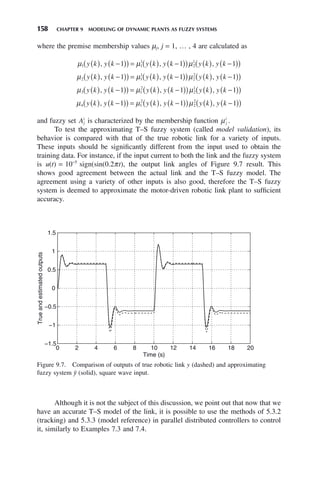
178. 160 CHAPTER 9 MODELING OF DYNAMIC PLANTS AS FUZZY SYSTEMS
When the RLS algorithm (8.7) with θ(0) = [0 0 0 0 0 0]T
and P(0) = 105
I is
run simultaneously with this system, the RLS parameter estimates converge after
∼5 s (i.e., after ∼500 steps) to
θ*
*
*
*
*
*
*
=
⎡
⎣
⎢
⎢
⎢
⎢
⎢
⎢
⎢
⎤
⎦
⎥
⎥
⎥
⎥
⎥
⎥
⎥
=
a
a
a
b
b
b
1
2
3
1
2
3
0 9926
1 0077
0 9901
.
.
.
2
2 1176 10
1 4328 10
1 8814 10
5
5
5
.
.
.
×
− ×
×
⎡
⎣
⎢
⎢
⎢
⎢
⎢
⎢
⎢
⎤
⎦
⎥
⎥
⎥
⎥
⎥
⎥
⎥
−
−
−
This results in the following T–S fuzzy rule base:
1. If y(k) is Al
, then ŷ1
(k + 1) = 0.9926y(k) + 2.1176 × 10−5
u(k).
2. If y(k) is A2
, then ŷ2
(k + 1) = 1.0077y(k) − 1.4328 × 10−5
u(k).
3. If y(k) is A3
, then ŷ3
(k + 1) = 0.9901y(k) + 1.8814 × 10−5
u(k).
This rule base together with the input memberships in Figure 9.8 constitute
the T–S fuzzy system to closely match the system (9.10). The output of the fuzzy
approximator closely matches that of the true system for a variety of inputs, hence
the approximator is deemed valid.
Once again, we point out that with the above fuzzy approximation it is now
possible to design tracking and model reference controllers for this plant.
9.2.3 Gradient Identification in Input–Output Difference
Equation Form
As discussed in Section 8.6, gradient identification does not need linearity in the
parameters. Therefore the input fuzzy sets, as well as the output parameters, can be
adjusted. Let the fuzzy approximator have R rules of the form:
Figure 9.8. Input memberships for fuzzy system approximating the nonlinear system of
(9.10).
−2 −1 0 1 2
0
0.2
0.4
0.6
0.8
1
y(k)
Membership
μ
A1
A2
A3

179. EXAMPLE 9.4 161
R y k A y k A y k n is A
y k
i
i i
n
i
i
: If is and is and and , then
( ) −
( ) − +
( )
+
1 2
1 1
1 1 1
1
1 2
1 2
( ) = ( )+ −
( ) + + − +
( )+
( )+ −
( ) + +
a y k a y k a y k n
b u k b u k b
i i
n
i
i i
n
n
i
u k n
− +
( )
1
(9.11)
Notice that these rules are in the form depicted in Figure 8.15, that is, Aj
i
is the
unique fuzzy set for Rule i, jth universe. The fuzzy system is described by (9.6),
where
ξ
μ
μ
i
i
i
y k y k y k n
y k y k n
y k y k
( ) −
( ) − +
( )
( ) =
( ) − +
( )
( )
( ) −
, , ,
, ,
, ,
1 1
1
n
n
i
R
+
( )
( )
=
∑ 1
1
(9.12)
and
μ
σ
i
j
i
j
i
j
n
y k y k n
y k j c
( ) − +
( )
( ) = −
− +
( )−
⎛
⎝
⎜
⎞
⎠
⎟
⎛
⎝
⎜
⎞
⎠
⎟
=
, , exp
1
1
2
1
2
1
∏
∏ (9.13)
Let the instantaneous estimation error be defined as
e k y k y k
( ) = +
( )− +
( )
[ ]
1
2
1 1
2
ˆ (9.14)
We seek to reduce e(k) by choice of parameters θ σ
c a b
j
i
j
i
j
i
j
i
, , ,
( ). Use c k
j
i
( ), σ j
i
k
( ),
a k
j
i
( ), b k
j
i
( ) to denote these parameters’ values at time k. By a process similar to
that of Sections 8.5 and 8.6, we derive the gradient update laws for these:
c k c k k
y k y k
y k y k n
j
i
j
i
i
i
i
+
( ) = ( )− ( )
+
( )− +
( )
( ) − +
( )
( )
1
1 1
1
1
λ ε
μ
ˆ ˆ
, ,
=
=
∑
⎛
⎝
⎜
⎜
⎜
⎜
⎞
⎠
⎟
⎟
⎟
⎟
⋅
( ) − +
( )
( )
− +
( )− ( )
( )
1
1
1
R
i
j
i
j
i
y k y k n
y k j c k
k
μ
σ
, ,
( )
⎛
⎝
⎜
⎞
⎠
⎟
2
(9.15a)
σ σ λ ε
μ
j
i
j
i
i
i
i
k k k
y k y k
y k y k n
+
( ) = ( )− ( )
+
( )− +
( )
( ) − +
( )
( )
1
1 1
1
2
ˆ ˆ
, ,
=
=
∑
⎛
⎝
⎜
⎜
⎜
⎜
⎞
⎠
⎟
⎟
⎟
⎟
⋅
( ) − +
( )
( )
− +
( )− ( )
( )
1
2
1
1
R
i
j
i
j
i
y k y k n
y k j c k
μ
σ
, ,
k
k
( )
( )3
(9.15b)
a k a k k
y k y k n
y k y k n
j
i
j
i i
j
+
( ) = ( )− ( )
( ) − +
( )
( )
( ) − +
( )
1
1
1
3
λ ε
μ
μ
, ,
, ,
(
( )
− +
( )
=
∑
j
R
y k j
1
1 (9.15c)
b k b k k
y k y k n
y k y k n
j
i
j
i i
j
+
( ) = ( )− ( )
( ) − +
( )
( )
( ) − +
( )
1
1
1
4
λ ε
μ
μ
, ,
, ,
(
( )
− +
( )
=
∑
j
R
u k j
1
1 (9.15d)

180. 162 CHAPTER 9 MODELING OF DYNAMIC PLANTS AS FUZZY SYSTEMS
EXAMPLE 9.5
Consider the gantry of Section 1.4, which is a nonminimum-phase nonlinear system.
The truth model for the gantry is given by
ψ
ψ ψ ψ ψ
ψ
=
− + − +
( )
+
9 81 1 76 0 18
0 9 0 3
2
2
. sin . cos . sin
. . cos
u
(9.16)
where ψ is the angle of the rod from vertical-down, u(t) is the input force
delivered to the cart, and the output y = ψ. The system is simulated with a
fourth-order Runge–Kutta integration algorithm with a step size of 0.01 s. For the
input–output data, we measure pairs {u(kΔt), y(kΔt)} for k = 1, 2, 3, … and
Δt = 0.01 s.
The input signal chosen for the identification consists of six frequencies cover-
ing the operating frequency range of the gantry:
u t t t t t t
( ) = + + + + +
1 3 0 01 0 02 0 05 0 1 0 2
. sin . sin . sin . sin . sin . si
π π π π π n .
0 5πt
( )
A fuzzy system with1 input and 50 rules is found to be sufficient to accurately
approximate the system. Thus there are 200 unknown parameters to be determined
via gradient: 50 c’s, 50 σ ’s, 50 a’s, and 50 b’s. The step sizes chosen by trial and
error are λ1 = λ2 = 5, λ3 = λ4 = 0.5. After 105
iterations through the gradient algo-
rithm, the parameters have converged to constant values. The resulting 50-rule T–S
fuzzy system produces close agreement with the truth model (9.16) for a variety of
inputs. An example is shown in Figure 9.9, where the test input is
u t t t t
( ) = ( )+ ( )+ ( )
sin . sin . sin .
1 5 0 85 0 15
π π π (9.17)
Figure 9.9. Comparison of gantry output and gradient-trained T–S fuzzy model output for
test input (9.17).
0 2 4 6 8 10 12 14 16 18 20
−1.5
−1
−0.5
0
0.5
1
1.5
Time (s)
Output
(rad)
Gantry angle
Model output

181. 9.3 IDENTIFICATION IN COMPANION FORM 163
9.3 IDENTIFICATION IN COMPANION FORM
A continuous-time feedback linearizable system can be modeled in companion form
(see Section 5.1.1)
y x x u
m
( )
= ( )+ ( )
δ η (9.18)
where y(m)
= dm
y/dtm
, x is the vector of states, and m is the relative degree of the
system. If the system is unknown, it can be estimated by estimating the nonlinear
functions δ(x) and η(x) by fuzzy systems fδ (x) and fη(x):
y f x f x u
m
( )
≈ ( )+ ( )
δ η (9.19)
9.3.1 Least-Squares Identification in Companion Form
If fδ (x) and fη(x) are estimated using least squares (Sections 8.1 or 8.2), the
input membership functions must be fixed and the locations of the output singletons
are adjustable. Let the rule base of the fuzzy system fδ consist of R rules of
the form
R x A x A x A f a
i
K L
n n
M i
: ,
If is and is and and is then is
1 1 2 2
δ δ δ
δ
(9.20)
and the rule base of the fuzzy system fη consist of S rules of the form
R x A x A x A f b
i
K L
n n
M i
: ,
If is and is and and is then is
1 1 2 2
η η
η
η
(9.21)
Then,
f x ai
i
i
R
δ ξ
( ) =
=
∑
1
(9.22)
and
f x bi
i
i
S
η ζ
( ) =
=
∑
1
(9.23)
where ξi, i = 1, … , R are the fuzzy basis functions
ξ
μ
μ
i
i
i
i
R
x
x
x
( ) =
( )
( )
=
∑
1
(9.24)
with μi(x) the premise membership function of the ith rule of fuzzy system fδ, ζi,
i = 1, … , S are the fuzzy basis functions
ζ
ν
ν
i
i
i
i
S
x
x
x
( ) =
( )
( )
=
∑
1
(9.25)
with vi(x) the premise membership function of the ith rule of fuzzy system fη, and
ai
, i = 1, … , R, bi
, i = 1, … , S are unknown parameters to be adjusted by least
squares.

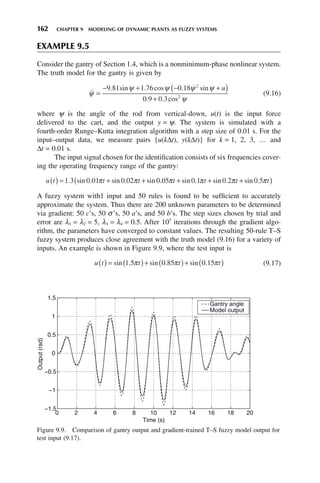
182. 164 CHAPTER 9 MODELING OF DYNAMIC PLANTS AS FUZZY SYSTEMS
Now (9.19) can he written
y a b u
a a b u b u
m i
i
i
R
i
i
i
S
R
R
S
S
T
( )
= =
≈ +
= + + + + +
=
∑ ∑
ξ ζ
ξ ξ ζ ζ
φ θ
1 1
1
1
1
1
(9.26)
with
φ ξ ξ ζ ζ
T
R S
u u
= [ ]
1 1
and
θ = [ ]
a a b b
R S
1 1
T
Then, the unknown output parameters ai
and bi
contained in θ can be estimated via
batch or recursive least squares as follows.
Let data {x(k), u(k), y(m)
(k)}, k = 1, 2, 3, … be taken from the plant, where
y(m)
= dm
y/dtm
. Define
ξ
μ
μ
i
i
i
i
R
k
x k
x k
i R
( ) =
( )
( )
( )
( )
=
=
∑
1
1
, , ,
… (9.27)
ζ
ν
ν
i
i
i
i
S
k
x k
x k
i S
( ) =
( )
( )
( )
( )
=
=
∑
1
1
, , ,
… (9.28)
and
φ ξ ξ ζ ζ
T
k k k k u k k u k
R S
( ) = ( ) ( ) ( ) ( ) ( ) ( )
[ ]
1 1
(9.29)
For batch least squares, consider only M of the input–output measurements
{x(k), u(k), y(m)
(k)}, k = 1, … , M. Form matrices
Φ =
( )
( )
( )
⎡
⎣
⎢
⎢
⎢
⎢
⎤
⎦
⎥
⎥
⎥
⎥
× +
( )
φ
φ
φ
T
T
T
M
M R S
1
2
∼
and
Y y y y M M
m m m T
= ( ) ( ) ( )
⎡
⎣ ⎤
⎦ ×
( ) ( ) ( )
1 2 1
∼
Then, the batch least-squares estimate of θ based on the M measurements considered
is calculated as in (8.6), that is, θ̂* = ( )−
Φ Φ Φ
T T
Y
1
.
For recursive least squares, let the parameter estimate at time k be
ˆ ˆ ˆ ˆ ˆ
θ k a k a k b k b k
R S
( ) = ( ) ( ) ( ) ( )
⎡
⎣ ⎤
⎦
1 1
T

183. 9.3 IDENTIFICATION IN COMPANION FORM 165
Then the recursive least-squares algorithm proceeds as in (8.7) with a correction
term of y k k k
m T
( )
( )− ( ) −
( )
⎡
⎣ ⎤
⎦
φ θ̂ 1 . Therefore, it is necessary not only to know the
system’s relative degree m, but also to differentiate the system output m times.
Although signal differentiation is undesirable in practice, it is unavoidable in this
case. For the relative degree, one needs some idea of the system model. In most
cases, m is treated as a design parameter and determined by trial and error.
9.3.2 Gradient Identification in Companion Form
If fδ (x) and fη(x) are estimated using gradient (Sections 8.5), the input membership
functions, as well as the locations of the output singletons, are adjustable. Let the
rule base of the fuzzy system fδ consist of R rules of the form
1
2
1 1
1
2 2
1 1 1
1 1
2
. , .
.
If is and is and and is then is
If is
x A x A x A f a
x A
n n
δ
a
and is and and is then is
If is and is
x A x A f a
R x A x A
n n
R
2 2
2 2 2
1 1 2 2
, .
.
δ
R
R
n n
R R
x A f a
and and is then is
, .
δ
(9.30)
and the rule base of the fuzzy system fη consist of S rules of the form
1
2
1 1
1
2 2
1 1 1
1 1
2
. , .
.
If is and is and and is then is
If is
x B x B x B f b
x B
n n
η
a
and is and and is then is
If is and is
x B x B f b
S x B x B
n n
S
2 2
2 2 2
1 1 2 2
, .
.
η
S
S
n n
S S
x B f b
and and is then is
, .
η
(9.31)
For the rule base of (9.30), assuming we use Gaussian input membership functions,
the membership function characterizing Aj
i
(ith rule, jth universe) is given by
μ
σ
j
i
j
j j
i
j
i
x
x c
( ) = −
−
⎛
⎝
⎜
⎞
⎠
⎟
⎛
⎝
⎜
⎞
⎠
⎟
exp
1
2
2
(9.32)
Similarly, the membership function characterizing Bj
i
(ith rule, jth universe) is
given by
ν
ρ
j
i
j
j j
i
j
i
x
x d
( ) = −
−
⎛
⎝
⎜
⎞
⎠
⎟
⎛
⎝
⎜
⎞
⎠
⎟
exp
1
2
2
(9.33)
Using product T-norm, the premise value of Rule i of rule base (9.30) is
μ
σ
i n
j j
i
j
i
j
n
x x x
x c
1 2
2
1
1
2
, , , exp
( ) = −
−
⎛
⎝
⎜
⎞
⎠
⎟
⎛
⎝
⎜
⎞
⎠
⎟
=
∏ (9.34)
Then, the fuzzy system fδ’s input–output characteristic is given by

184. 166 CHAPTER 9 MODELING OF DYNAMIC PLANTS AS FUZZY SYSTEMS
f x
a
x c
x c
i j j
i
j
i
j
n
i
R
j j
δ θ
σ
( ) =
−
−
⎛
⎝
⎜
⎞
⎠
⎟
⎛
⎝
⎜
⎞
⎠
⎟
−
−
=
=
∏
∑ exp
exp
1
2
1
2
2
1
1
i
i
j
i
j
n
i
R
i
i
i
R
i
i
R
a x
x
σ
μ
μ
⎛
⎝
⎜
⎞
⎠
⎟
⎛
⎝
⎜
⎞
⎠
⎟
=
( )
( )
=
=
=
=
∏
∑
∑
∑
2
1
1
1
1
(9.35)
Similarly, the premise value of Rule i of rule base (9.31) is
ν
ρ
i n
j j
i
j
i
j
n
x x x
x d
1 2
2
1
1
2
, , , exp
( ) = −
−
⎛
⎝
⎜
⎞
⎠
⎟
⎛
⎝
⎜
⎞
⎠
⎟
=
∏ (9.36)
Then, the fuzzy system fη’s input–output characteristic is given by
f x
b
x d
x d
i j j
i
j
i
j
n
i
S
j j
η θ
ρ
( ) =
−
−
⎛
⎝
⎜
⎞
⎠
⎟
⎛
⎝
⎜
⎞
⎠
⎟
−
−
=
=
∏
∑ exp
exp
1
2
1
2
2
1
1
i
i
j
i
j
n
i
S
i
i
i
S
i
i
S
b x
x
ρ
ν
ν
⎛
⎝
⎜
⎞
⎠
⎟
⎛
⎝
⎜
⎞
⎠
⎟
=
( )
( )
=
=
=
=
∏
∑
∑
∑
2
1
1
1
1
(9.37)
Now, assume we are given the kth training data triple {x(k), u(k), y(m)
(k)}. Let
the instantaneous estimation error corresponding to this triple be defined as
e k f x k f x k u k y k
m
( ) = ( )
( )+ ( )
( ) ( )− ( )
⎡
⎣ ⎤
⎦
( )
1
2
2
δ η
θ θ (9.38)
We seek to reduce e(k) by choice of parameters θ σ ρ
a c b d
i
j
i
j
i i
j
i
j
i
, , , , ,
( ).
Use ai
(k), c k
j
i
( ) , σ j
i
k
( ) , bi
(k), d k
j
i
( ), ρj
i
k
( ) to denote these parameters’ values at
time k.
By a process similar to that of Sections 8.5 and 8.6, we derive the gradient
update laws for these, where ε = fδ (x(k)|θ) + fη(x(k)|θ)u(k) − y(m)
(k):
a k a k k
x k
x k
i i i
i
i
R
+
( ) = ( )− ( )
( )
( )
( )
( )
=
∑
1 1
1
λ ε
μ
μ
(9.39a)
c k c k k
a k f x k k
x k
j
i
j
i
i
i
i
R
+
( ) = ( )− ( )
( )− ( ) ( )
( )
( )
( )
⎛
⎝
⎜
⎜
⎜
=
∑
1 2
1
λ ε
θ
μ
δ
⎜
⎜
⎞
⎠
⎟
⎟
⎟
⎟
( )
( )
( )− ( )
( )
( )
⎛
⎝
⎜
⎞
⎠
⎟
μ
σ
i
j j
i
j
i
x k
x k c k
k
2
(9.39b)

185. 9.4 SUMMARY 167
σ σ λ ε
θ
μ
δ
j
i
j
i
i
i
i
R
k k k
a k f x k k
x k
+
( ) = ( )− ( )
( )− ( ) ( )
( )
( )
( )
⎛
⎝
⎜
⎜
⎜
=
∑
1 3
1
⎜
⎜
⎞
⎠
⎟
⎟
⎟
⎟
( )
( )
( )− ( )
( )
( )
( )
μ
σ
i
j j
i
j
i
x k
x k c k
k
2
3
(9.39c)
b k b k k u k
x k
x k
i i i
i
i
S
+
( ) = ( )− ( ) ( )
( )
( )
( )
( )
=
∑
1 4
1
λ ε
ν
ν
(9.39d)
d k d k k u k
b k f x k k
x k
j
i
j
i
i
i
i
S
+
( ) = ( )− ( ) ( )
( )− ( ) ( )
( )
( )
( )
⎛
=
∑
1 5
1
λ ε
θ
ν
η
⎝
⎝
⎜
⎜
⎜
⎜
⎞
⎠
⎟
⎟
⎟
⎟
⋅ ( )
( )
( )− ( )
( )
( )
⎛
⎝
⎜
⎞
⎠
⎟
ν
ρ
i
j j
i
j
i
x k
x k d k
k
2
(9.39e)
ρ ρ λ ε
θ
ν
η
j
i
j
i
i
i
i
S
k k k u k
b k f x k k
x k
+
( ) = ( )− ( ) ( )
( )− ( ) ( )
( )
( )
( )
⎛
=
∑
1 6
1
⎝
⎝
⎜
⎜
⎜
⎜
⎞
⎠
⎟
⎟
⎟
⎟
⋅ ( )
( )
( )− ( )
( )
( )
( )
ν
ρ
i
j j
i
j
i
x k
x k d k
k
2
3
(9.39f)
9.4 SUMMARY
In this chapter, the capabilities of fuzzy systems to estimate static nonlinear
functions are utilized for the identification of dynamic plants. This chapter discusses
two model forms for the estimated system: input–output difference equation
form and companion form. These are explored because they can he utilized in
parallel distributed controllers as in Chapter 7, and in Chapter 10 for adaptive fuzzy
control.
If the identification is done in input–output difference equation form, the
approximating fuzzy system is of the T–S type with consequents that are input–
output difference equations. This form of model can be used for tracking and model
reference controllers. If the identification is done in companion form, the fuzzy
approximator is a Mamdani fuzzy system whose consequents are unknown con-
stants. This form of model can be used for feedback linearization.
For both of these model forms, we discuss two methods of parameter estima-
tion: least squares and gradient. These are covered because they are recursive and
admit online control. Batch and recursive least-squares methods can only be used
for problems in which the system to be estimated is linear in the parameters.
Therefore, to be used for the construction of a fuzzy system, the input fuzzy sets
must be fixed a priori and only the consequent parameters can be adjusted. The
gradient method does not require the system to be linear in the parameters, therefore
both input and output fuzzy sets can be adjusted.

186. 168 CHAPTER 9 MODELING OF DYNAMIC PLANTS AS FUZZY SYSTEMS
EXERCISES
9.1 Show that the two-rule fuzzy system of Example 9.1 exactly duplicates the
system ẋ= z(x)x on the domain X, where b z
m = ( )
min
X
and b z
M = ( )
max
X
.
9.2 Completely specify a T–S fuzzy system to exactly duplicate the behavior of
the forced pendulum (5.4) on the interval −π/4 ≤ x1 ≤ π/4, −5 ≤ x2 ≤ 5.
9.3 Find a fuzzy system that is exactly equivalent to the system
x x u
= +
3
cos
on the interval −2 ≤ x ≤ 2.
9.4 In Example 9.3, assume the number of inputs is 3, the number of fuzzy sets
on each input universe is 3, and we have 500 input–output pairs available.
(a) How many rules are there? (b) How many unknown parameters are there?
(c) Sketch the membership functions characterizing all input fuzzy sets. (d)
What is the dimension of Φ? Y?
9.5 In Example 9.3, let a typical rule be
R y k A y k A
i
K L
: ,
If is and is then
( ) −
( )
1 2
1
ŷ k a y k a y k b u k b u k
i i i i i
+
( ) = ( )+ −
( )+ −
( )+ −
( )
1 1 1 2
1 2 1 2
Assume the number of fuzzy sets on each input universe is 2 and we have
200 input–output pairs available. Write the φ(k) and θ(k) vectors and give
their dimension.
9.6 In Example 9.4, let a typical rule be
R y k A y k a y k b u k
i
K i i i
: If is , then
( ) +
( ) = ( )+ ( )
1 1 1
and each input universe has 4 fuzzy sets. (a) How many rules are there? (b)
How many unknown parameters are there? (c) Specify Φ, Y, and θ and give
their dimensions. (d) Specify the RLS algorithm including all necessary initial
conditions.
9.7 Repeat Problem 9.5 if a typical rule is of the form:
R y k A y k A
i
K L
: ,
If is and is then
( ) −
( )
1 2
1
ŷ k a y k a y k b u k b u k
i i i i i
+
( ) = ( )+ −
( )+ −
( )+ −
( )
1 1 1 2
1 2 1 2
9.8 Consider the gantry of Example 9.5. (a) Is it feedback linearizable? If so,
what is its relative degree? (b) Write its model in companion form. (c) Is it
controllable? If so, for what ψ? How do you explain this range of ψ for
controllability in terms of the physical system?
9.9 Consider the gradient identification in companion form. Fuzzy systems fδ and
fη each have two inputs and three rules. Write gradient parameter update
equations for all adjustable parameters.
9.10 Derive the gradient update laws (9.15) and (9.39).

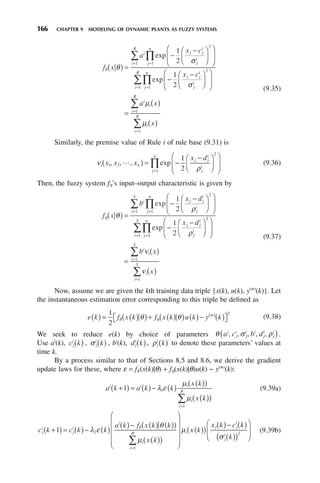
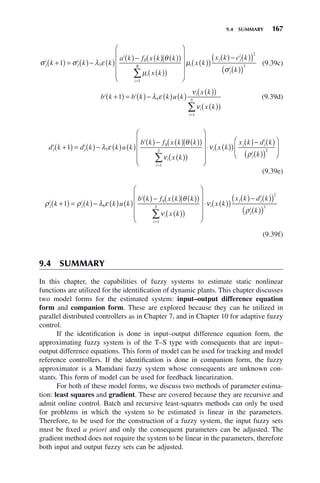
187. 169
Fuzzy Control and Identification, By John H. Lilly
Copyright © 2010 John Wiley Sons, Inc.
An adaptive controller is one that adjusts itself to changes in the plant it is control-
ling. For instance, consider a robotic arm carrying a load in its end manipulator
(hand) and being controlled by an adaptive tracking controller. The controller is
designed to force the arm to follow a prescribed reference trajectory through space
while moving the load from its start point to its destination. If the mass being moved
changes mid-trajectory (say the manipulator accidentally drops some of its load),
the controller, because it is adaptive, can adapt to this change and still obtain the
same tracking performance as before.
Adaptive controllers fall into two categories [27,33,36–39]: indirect and
direct. The approach in indirect adaptive control is to identify a model for the plant,
then to derive a controller based on this identified model. The controller calculation
is done simultaneously with the plant identification, so model and controller evolve
together.
This is called the certainty equivalence principle: at each point in the evolu-
tion, the controller design is based on the current plant estimate. It is assumed
that, as the estimated plant model gets more accurate, the controller also gets more
accurate and, in the limit, perfect control is obtained. Furthermore, since the
identifier and controller run continuously, if the plant changes in some way (like the
robotic arm dropping part of its load in the example above) the estimated model and
corresponding controller change correspondingly resulting in a new perfect control.
In direct adaptive control, the controller is adjusted directly without referring
to any plant model. Thus, the indirect step of identifying the plant is avoided. Instead,
the controller adjustment is made on the basis of an error that rates the closed-loop
performance.
Plants controlled by adaptive controllers (even nonfuzzy ones) give rise to
complex time-varying nonlinear closed-loop systems, whose stability is difficult or
impossible to verify. During the last three decades, researchers have met with some
success in proving stability of some closed-loop systems containing adaptive con-
trollers. But if the controller is fuzzy, closed-loop stability is much more difficult to
prove due to the complexity of fuzzy systems. Therefore, none of the techniques
presented in this chapter have been proven to work in all situations, although they
may work well in many.
ADAPTIVE FUZZY CONTROL
CHAPTER 10

188. 170 CHAPTER 10 ADAPTIVE FUZZY CONTROL
Adaptive controllers run online continuously. Therefore, for indirect adaptive
controllers, only recursive parameter estimation algorithms can be used. In Chapters
8 and 9, the only recursive algorithms presented are recursive least-squares (RLS)
and gradient. Therefore, we only discuss these two algorithms in connection with
indirect adaptive fuzzy control.
10.1 DIRECT ADAPTIVE FUZZY TRACKING
CONTROL [12]
Consider the single-input, single-output plant
x f g u
p
n
p p
( )
= + (10.1a)
y h x
p p p
= (10.1b)
where x(n)
:= dn
x/dtn
, fp, gp, and hp are unknown scalar functions of the plant state
x x x x
p p p
n
= [ ]
−
( )
, , ,
1
and gp 0 is bounded away from zero. The control objective
is to find a plant input, u such that yp(t) asymptotically tracks a bounded reference
signal r(t).
Define the tracking error er = r − yp, an error vector εr r r r
n T
e e e
= [ ]
−
( )
1
,
and constants k1, … , kn, such that the roots of sn
+ k1sn−1
+ … + kn−1s + kn are all in
the open left half-plane. Define the companion matrix
Λ =
− − − − −
⎡
⎣
⎢
⎢
− − −
0 1 0 0 0
0 0 1 0 0
0 0 0 1 0
0 0 0 0
1
1 2 3 1
k k k k k
n n n n
⎢
⎢
⎢
⎢
⎢
⎢
⎤
⎦
⎥
⎥
⎥
⎥
⎥
⎥
⎥
(10.2)
Let pn be the last column of the positive definite matrix P satisfying the Lyapunov
matrix equation
Λ Λ
T
P P Q
+ = − (10.3)
where Q is a symmetric positive-definite matrix.
Let the inputs to the fuzzy system be x x x x x x
n p p p
n
1 2
1
, , , , , ,
… …
[ ]= [ ]
−
( )
and
define fuzzy sets Ai
j
, i = 1, … , n, j = 1, … , m on each universe of discourse. Let
the rule base of the direct adaptive fuzzy tracking controller consist of mn
rules of
the form
R x A x A x A t
i
j k
n n
l i
i
: ,
If is and is and and is then is
1 1 2 2 θ θ ( ) (10.4)
Let ξi(x) be the fuzzy basis function for Rule i [in (10.4)] and define ξ ξ ξ ξ
= [ ]
1 2
, , ,
mn .
Defining the parameter vector θ θ θ θ
= [ ]
1 2
, , mn , the control law is given by
u x x t
θ ξ θ
( ) = ( ) ( ) (10.5)

189. EXAMPLE 10.1 DIRECT ADAPTIVE FUZZY TRACKING CONTROL FOR BALL AND BEAM 171
where the parameter vector θ(t) is adjusted according to
θ γε ξ
t p x
r
T
n
( ) = ( ) (10.6)
where γ 0 is an arbitrary constant.
Thus the consequents of the fuzzy rules are adjusted online according to (10.6) at
each time step.
Note that there is an added supervisory control in [12] guaranteeing bounded-
ness of all signals in the closed-loop system and convergence of er(t) to 0 as t → ∞.
This is not addressed here. Such guarantees are usually not available for closed-loop
systems containing fuzzy controllers, especially adaptive ones.
EXAMPLE 10.1 DIRECT ADAPTIVE FUZZY TRACKING
CONTROL FOR BALL AND BEAM
Consider the ball and beam with a time-varying friction (Fig. 1.3) modeled by
mx x g
= − + ( )
ν ψ
2 sin (10.7)
where x is the ball’s position on the beam with x = 0 corresponding to the middle
of the beam, m = 1kg is the ball’s mass, ν is the friction encountered by the ball in
its travel, g = 9.81m/s2
is the acceleration of gravity, and ψ is the beam angle in
radians. Define the plant output yp = x.
The inputs to the direct adaptive fuzzy tracking controller are x and ẋ.
Define three fuzzy sets Ax
1
, Ax
2
, Ax
3
on the x universe and three fuzzy sets Ax
1
, Ax
2
,
Ax
3
on the ẋ universe (see Fig. 10.1). Therefore the fuzzy controller consists
of 32
= 9 rules.
Figure 10.1. Input fuzzy sets on x and ẋ universes.
0
0.2
0.4
0.6
0.8
1
x and dx/dt
Membership
μ
A1
A2
A3
0
−π/2 π/2

190. 172 CHAPTER 10 ADAPTIVE FUZZY CONTROL
Let k1 = 2 and k2 = 1, so that s2
+ 2s + 1 = (s + 1)2
has both roots in the open
left half-plane. Define Q = diag(1, 10). Then the solution to (10.3) is the positive
definite symmetric matrix
P =
⎡
⎣
⎢
⎤
⎦
⎥
3 75 0 5
0 5 2 75
. .
. .
(10.8)
giving p2 = [0.5 2.75]T
. The error vector is εr = [r − yp ṙ − ẏp]T
. Setting γ = 10,
the adaptive law (10.6) is given by
θ ε ξ
i r
T
i
p x
= ( )
10 2 , i = 1, … , 9 or
…
θ ξ
i p p i
r y r y x i
= −
( )+ −
( )
[ ] ( ) =
10 0 5 2 75 1 2 9
. . , , , , (10.9)
where the fuzzy basis function ξi(x) corresponds to Rule i in the rule base:
1
2
1 1 1
1
1 2
. , .
. ,
If is and is then
If is and is t
x A x A t
x A x A
x x
x x
θ θ
= ( )
h
hen
If is and is then
If is
θ θ
θ θ
2
2
1 3 3
3
2
3
4
= ( )
= ( )
t
x A x A t
x A
x x
x
.
. , .
.
a
and is then
If is and is then
x A t
x A x A t
x
x x
1 4
4
2 2 5
5
5
, .
. ,
θ θ
θ θ
= ( )
= (
( )
= ( )
.
. , .
.
6
7
2 3 6
6
3
If is and is then
If is and is
x A x A t
x A x A
x x
x
θ θ
x
x
x x
t
x A x A t
x
1 7
7
3 2 8
8
8
9
, .
. , .
.
then
If is and is then
If i
θ θ
θ θ
= ( )
= ( )
s
s and is then
A x A t
x x
3 3 9
9
, .
θ θ
= ( )
(10.10)
Finally, the control law is given by (10.5).
The reference input
r t t t
( ) = +
0 5 0 1 0 3 0 4
. sin . . sin .
π π (10.11)
with x(0) = 1 and a friction that varies as
ν t
t
t
( ) =
≤
≤
⎧
⎨
⎩
4 0 30
0 30 60
,
,
s
s
(10.12)
results in the tracking performance shown in Figure 10.2, where the simulation is
done using a fourth-order Runge–Kutta integration routine. Note that, because
the controller is adaptive, the tracking accuracy is not adversely affected when
the friction changes abruptly at t = 30s. The controller simply adapts itself to this
change (the θ ’s change) and tracking is resumed after a brief period of
readaptation.

191. EXAMPLE 10.2 DIRECT ADAPTIVE FUZZY MODEL REFERENCE CONTROL 173
10.2 DIRECT ADAPTIVE FUZZY MODEL
REFERENCE CONTROL
One version of the model reference control problem is to force the plant output to
track the output of a reference model
x f g r
m
n
m m
( )
= + (10.13a)
y h x
m m m
= (10.13b)
where fm, gm, hm are known scalar functions of the model states x x x x
m m m
n
= ⎡
⎣ ⎤
⎦
−
( )
, , ,
… 1
and r(t) is the model input. The derivation of the model reference controller is identi-
cal to that of the tracking controller (Section 10.1) except we now define the model
following error em = ym − yp and error vector εm m m m
n T
e e e
= [ ]
−
( )
, , ,
… 1
.
EXAMPLE 10.2 DIRECT ADAPTIVE FUZZY MODEL
REFERENCE CONTROL FOR BALL AND BEAM
Consider the ball and beam with a time-varying friction modeled by (10.7),
where again yp = x. The inputs to the fuzzy direct adaptive model reference controller
are x and ẋ. Define three fuzzy sets Ax
1
, Ax
2
, Ax
3
on the x universe and three fuzzy
sets Ax
1
, Ax
2
, Ax
3
on the ẋ universe (see Fig. 10.1). Therefore the fuzzy controller
has 9 rules. Let k1 = 2, k2 = 1, and Q = diag(1, 10) as before, again giving
p2 = [0.5 2.75]T
.
Figure 10.2. Tracking performance of direct adaptive fuzzy tracking controller, friction
changing at t = 30s.
0 10 20 30 40 50 60
−1
−0.5
0
0.5
1
1.5
Time (s)
Ball
position
(m)
r(t)
yp
(t)

192. 174 CHAPTER 10 ADAPTIVE FUZZY CONTROL
Define the reference model
x x r
m m
=
− −
⎡
⎣
⎢
⎤
⎦
⎥ +
⎡
⎣
⎢
⎤
⎦
⎥
0 1
1 10
0
3
(10.14a)
y x
m m
= [ ]
1 0 (10.14b)
The model reference error vector is εm = [ym − yp ẏm − ẏp]T
. Setting γ = 10,
the adaptive law is given by
θ ε ξ
i m
T
i
p x
= ( )
10 2 , i = 1, … , 9 or
…
θ ξ
i m p m p i
y y y y x i
= −
( )+ −
( )
[ ] ( ) =
10 0 5 2 75 1 9
. . , , , (10.15)
where the fuzzy basis function ξi(x) corresponds to Rule i in the rule base given in
(10.10).
The reference input (10.11) applied to the reference model (10.14) with
x(0) = 1 and a plant friction that varies as (10.12) results in the tracking performance
shown in Figure 10.3, where the simulation is done using a fourth-order Runge–
Kutta integration routine. Note that, because the controller is adaptive, the tracking
accuracy is not adversely affected when the friction changes abruptly at t = 30s.
The controller simply adapts itself to this change (the θ’s change) and tracking is
resumed after a brief period of readaptation.
Figure 10.3. Tracking performance of direct adaptive fuzzy model reference controller,
friction changing at t = 30s.
0 10 20 30 40 50 60
−0.6
−0.4
−0.2
0
0.2
0.4
0.6
0.8
1
Time (s)
Ball
position
(m)
ym
(t)
yp
(t)
Here, we have given one idea for direct adaptive fuzzy control. An interesting
idea called fuzzy model reference learning control (FMRLC) is another well-known
type of direct adaptive fuzzy control. The FMRLC goes beyond what is presented
here in that the controller not only learns but remembers what it has learned. Thus
it is slightly more involved than what we have presented here. The interested reader
is referred to [9,40] for more information on FMRLC.

193. EXAMPLE 10.3 INDIRECT ADAPTIVE FUZZY TRACKING CONTROL FOR GANTRY 175
10.3 INDIRECT ADAPTIVE FUZZY
TRACKING CONTROL
As discussed in Sections 9.2.2 and 9.2.3, recursive least squares or gradient can be
used to recursively identify a T–S fuzzy model for any time-invariant system. The
T–S fuzzy system (called the plant fuzzy system) has rules of the form (9.4), that is,
the rule consequents are input–output difference equations. At each time step, the
parameter estimates in the consequents change and eventually converge to constant
values.
Section 7.3 shows how to design a parallel distributed tracking controller for
a time-invariant system modeled as a T–S fuzzy system with rules of the form (9.4).
Using the certainty equivalence principle at each time step, we can employ this
design method to derive a parallel distributed tracking controller (called the control-
ler fuzzy system). The parameters of the controller fuzzy system change at each time
step in response to the changing parameters in the plant fuzzy system. If the
identification–control design process described above is left running online, the
controller can adapt to any change in the plant being controlled and still produce
accurate tracking even in the presence of such change.
In contrast to direct adaptive control, the indirect adaptive control strategy
takes the additional step of identifying a model for the plant. In fact, this is one of
the advantages of the indirect control strategy: A plant model is obtained as a
byproduct of the control method. Note, however, that we are not as interested in
accurately identifying the plant as in controlling it, although acquiring an accurate
plant model is certainly a valuable byproduct.
EXAMPLE 10.3 INDIRECT ADAPTIVE FUZZY
TRACKING CONTROL FOR GANTRY
(RLS PARAMETER ADAPTATION)
Consider the gantry of Example 9.5 whose truth model (assumed unknown) is given
by (9.16), where ψ is the angle of the rod from vertical-down, u(t) is the input force
delivered to the cart, and the output y = ψ. It is desired to formulate a force input
to the cart so that the pendulum angle tracks the reference signal
r t t t t
( ) = + +
( )
0 2 0 5 0 7 2
. sin . sin . sin
π π π (10.16)
Since the gantry model is unknown, we use recursive least-squares parameter esti-
mation to identify it together with a certainty-equivalent parallel distributed adaptive
tracking control strategy.
Through trial and error, it is determined that a Takagi–Sugeno (T–S) fuzzy
system with two inputs (y(k) and y(k − 1)) and four fuzzy sets characterized by
triangular membership functions forming partitions of unity on [−π/2, π/2] on each
universe ( Aj
i
, j = 1, 2, i = 1, 2, 3, 4) is sufficient to accurately control the system.

194. 176 CHAPTER 10 ADAPTIVE FUZZY CONTROL
The memberships characterizing the input fuzzy sets are shown in Figure 10.4.
Therefore, there are 16 rules and 64 parameters to be identified.
Figure 10.4. Input fuzzy sets on y(k) and y(k − 1) universes.
0
0.2
0.4
0.6
0.8
1
y(k) and y(k−1)
Membership
μ
A1
A2
A3
A4
−π/2 −π/6 π/6 π/2
0
For the RLS algorithm initial conditions, we set P(0) = 105
I64 and θi(0) = 0.001,
i = 1, … , 64. The step size of the RK4 routine used for the simulation is 0.01s. A
typical rule in the rule base of the plant fuzzy system is
Rip: If y(k) is Ai
1 and y(k − 1) is Ai
2, then
ˆ ˆ ˆ ˆ ˆ
y k a y k a y k b u k b u k
i i i i i
+
( ) = ( )+ −
( )+ ( )+ −
( )
1 1 1
1 2 1 2
and a typical rule in the rule base of the controller fuzzy system is
Ric: If y(k) is Ai
1 and y(k − 1) is Ai
2 , then
u k
b k
b u k a y k a y k r k
i
i
i i i
( ) =
( )
− −
( )− ( )− −
( )+ +
( )
⎡
⎣ ⎤
⎦
1
1 1 1
1
2 1 2
ˆ
ˆ ˆ ˆ
Because of the 1 1
b̂ k
i
( ) term in the consequent of the controller fuzzy system, it is
necessary to insure that b̂ k
i
1 ( ) is bounded away from zero for all k to avoid division
by zero.
The tracking performance of the closed-loop system consisting of the gantry
and the indirect adaptive tracking controller is shown in Figure 10.5. After an adap-
tation period of ∼8s, the rod angle tracks the reference signal well.

195. EXAMPLE 10.4 INDIRECT ADAPTIVE FUZZY TRACKING CONTROL 177
EXAMPLE 10.4 INDIRECT ADAPTIVE FUZZY TRACKING
CONTROL FOR MOTOR-DRIVEN ROBOTIC LINK
(GRADIENT PARAMETER ADAPTATION)
Consider the motor-driven robotic link shown in Figure 10.6, whose truth model
(assumed unknown) is given by
I mgl B
ψ ψ ψ τ
= − − +
cos (10.17)
where ψ is the link angle from horizontal in radians, m = 1kg is the mass of the
link, l = 0.25m is the distance from the motor shaft to the link’s center of mass,
I = ml2
(kg-m2
) is the rotational inertia of the shaft and load, B = 0.7kg-m2
/s is
the rotational friction of the motor shaft, g = 9.81m/s2
is the acceleration of gravity,
and τ (kg-m2
/s2
) is the torque delivered to the link by the motor. The output is the
measured link angle y(t) = ψ(t).
Figure 10.6. Robotic link of Example 10.5.
Link m,l
Motor
t
y
0°
Figure 10.5. Tracking performance of indirect adaptive fuzzy tracking controller for
gantry, RLS parameter adaptation.
0 5 10 15 20 25 30
−1
−0.5
0
0.5
1
1.5
Time (s)
Gantry
angle
(rad)
r(t)
y(t)

196. 178 CHAPTER 10 ADAPTIVE FUZZY CONTROL
It is desired to determine the torque to be delivered by the motor so that the
link angle tracks the reference signal
r t t t t
( ) = + +
( )
0 1 3 0 4 2 0 6 2 0 8
. sin . sin . sin .
π π π (10.18)
Since the plant model is unknown, we use gradient parameter estimation to recur-
sively identify it together with a certainty-equivalent parallel distributed adaptive
tracking control strategy.
Through trial and error, it is determined that a T–S fuzzy system with one
input (y(k)) and four rules is sufficient to accurately control the system. The plant
fuzzy system’s rule base is given by
1. If y(k) is A1
, then ŷ1
(k + 1) = a1
y(k) + b1
u(k).
2. If y(k) is A2
, then ŷ2
(k + 1) = a2
y(k) + b2
u(k).
3. If y(k) is A3
, then ŷ3
(k + 1) = a3
y(k) + b3
u(k).
4. If y(k) is A4
, then ŷ4
(k + 1) = a4
y(k) + b4
u(k).
where input fuzzy sets A1
, A2
, A3
, and A4
are characterized by Gaussian membership
functions whose centers and spreads are to be determined via gradient parameter
adaptation. In all, there are 16 parameters to be identified: four input membership
function centers (ci
, i = 1, 2, 3, 4), four input membership spreads (σi
, i = 1, 2, 3,
4), and eight consequent parameters (ai
and bi
, i = 1, 2, 3, 4). These are adjusted as
in (9.15), giving ĉi
(k), σ̂i
k
( ) , âi
(k), b̂i
(k), i = 1, 2, 3, 4 and all integer k.
At each time increment, the certainty equivalent tracking controller fuzzy
system is given by
1. If y(k) is A1
, then u1
(k) = (1/b̂1
)(−â1
y(k) + r(k + 1)).
2. If y(k) is A2
, then u2
(k) = (1/b̂2
)(−â2
y(k) + r(k + 1)).
3. If y(k) is A3
, then u3
(k) = (1/b̂3
)(−â3
y(k) + r(k + 1)).
4. If y(k) is A4
, then u4
(k) = (1/b̂4
)(−â4
y(k) + r(k + 1)).
The resulting torque delivered to the link at time k is
u k k u k k u k k u k k u k
( ) = ( ) ( )+ ( ) ( )+ ( ) ( )+ ( ) ( )
ξ ξ ξ ξ
1
1
2
2
3
3
4
4
where the fuzzy basis functions are given by
ξ
μ
μ μ μ μ
i
i
k
y k
y k y k y k y k
i
( ) =
( )
( )
( )
( )+ ( )
( )+ ( )
( )+ ( )
( )
=
1 2 3 4
1 2 3 4
, , ,
and the premise value of Rule i is given by
μ
σ
i
i
i
y k
y k c k
k
i
( )
( ) = −
( )− ( )
( )
⎛
⎝
⎜
⎞
⎠
⎟
⎛
⎝
⎜
⎞
⎠
⎟ =
exp , , ,
1
2
1 2 3 4
2
ˆ
ˆ
The gradient algorithm step sizes for the simulation are chosen as
λ1 = λ2 = λ3 = λ4 = 3 × 10−2
. The step size of the RK4 routine used for the simula-
tion is 0.01s.
To illustrate the adaptive capabilities of this controller, let the mass actuated
by the link change from 1 to 5kg at t = 30s, simulating an extra load being added
to the link. The tracking performance of the closed-loop system consisting of the
robotic link and the indirect adaptive tracking controller is shown in Figure 10.7.

197. EXAMPLE 10.5 INDIRECT ADAPTIVE FUZZY MODEL REFERENCE CONTROL 179
After an adaptation period of ∼20s, the rod angle tracks the reference signal well.
Note that increasing the load fivefold at t = 30s does result in a slight degradation
in tracking performance. Nevertheless, approximate tracking is retained even after
such a drastic increase in load mass. This is because the adaptive nature of the
controller allows it to adjust itself to the new operating conditions.
10.4 INDIRECT ADAPTIVE FUZZY MODEL
REFERENCE CONTROL
Assume the plant is modeled recursively as a T–S fuzzy system with rules of the form
(9.4). Section 7.4 shows how to design a parallel distributed model reference control-
ler for such a T–S fuzzy system. Using the certainty equivalence principle at each time
step, we can employ this design technique to derive a parallel distributed model refer-
ence controller for the plant. The parameters of the controller fuzzy system change at
each time step in response to the changing parameters in the plant fuzzy system.
If the identification–control design process described above is left running
online, the controller can adapt to any change in the plant being controlled and still
produce accurate tracking even in the presence of such change.
EXAMPLE 10.5 INDIRECT ADAPTIVE FUZZY MODEL
REFERENCE CONTROL FOR MOTOR-DRIVEN
ROBOTIC LINK (RLS PARAMETER ADAPTATION)
Consider the motor-driven robotic link shown in Figure 10.8, whose truth model
(assumed unknown) is given by
Figure 10.7. Tracking the performance of a robotic link controlled by an indirect adaptive
fuzzy controller with gradient parameter adaptation, link mass increasing fivefold at t = 30s.
0 10 20 30 40 50 60
−1.5
−1
−0.5
0
0.5
1
1.5
Time (s)
Link
angle
(rad)
r(t)
y(t)

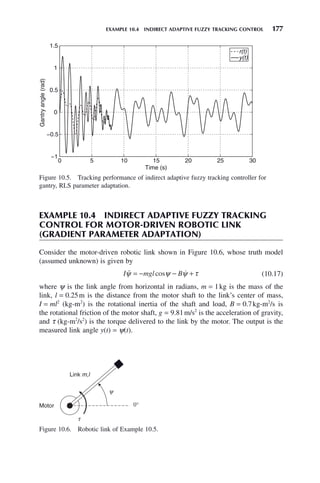
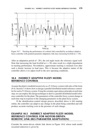
198. 180 CHAPTER 10 ADAPTIVE FUZZY CONTROL
ψ ψ ψ τ
= − − +
64 5 4
sin (10.19)
where ψ is the link angle from vertical-down in radians and τ is the torque delivered
to the link by the motor. The output is the measured link angle y(t) = ψ(t).
Figure 10.8. Robotic link of Example 10.5.
Motor
Link m, l
It is desired that the robotic link plant follow a model with transfer function
H z
z
z z
( ) =
−
− +
0 8
1 9 0 9125
2
.
. .
(10.20)
Thus in the notation of Section 5.3.3 we have g = 1, H(q−1
) = 1 − 0.8q−1
, and
E(q−1
) = 1 − 1.9q−1
+ 0.9125q−2
. Therefore, the reference model can be characterized
by the difference equation
y k y k y k r k r k
m m m
+
( ) = ( )− −
( )+ ( )− −
( )
1 1 9 0 9125 1 0 8 1
. . . (10.21)
where r(k) is an arbitrary reference input.
Through trial and error, it is determined that a T–S fuzzy system with two
inputs [y(k) and y(k − 1)] and three fuzzy sets characterized by triangular member-
ship functions forming partitions of unity on [−π/2, π/2] on each universe ( Aj
i
, j = 1,
2, i = 1, 2, 3) is sufficient to accurately control the system. The memberships char-
acterizing the input fuzzy sets are shown in Figure 10.9. Therefore, there are 9 rules
and 36 parameters to be identified.
The plant fuzzy system’s rule base is given by
1. If y(k) is A1
1
and y(k − 1) is A2
1
, then
ŷ k a y k a y k b u k b u k
1
1
1
2
1
1
1
2
1
1 1 1
+
( ) = ( )+ −
( )+ ( )+ −
( )
2. If y(k) is A1
1
and y(k − 1) is A2
2
, then
ŷ k a y k a y k b u k b u k
2
1
2
2
2
1
2
2
2
1 1 1
+
( ) = ( )+ −
( )+ ( )+ −
( )
3. If y(k) is A1
1
and y(k − 1) is A2
3
, then
ŷ k a y k a y k b u k b u k
3
1
3
2
3
1
3
2
3
1 1 1
+
( ) = ( )+ −
( )+ ( )+ −
( )

199. EXAMPLE 10.5 INDIRECT ADAPTIVE FUZZY MODEL REFERENCE CONTROL 181
4. If y(k) is A1
2
and y(k − 1) is A2
1
, then
ŷ k a y k a y k b u k b u k
4
1
4
2
4
1
4
2
4
1 1 1
+
( ) = ( )+ −
( )+ ( )+ −
( )
5. If y(k) is A1
2
and y(k − 1) is A2
2
, then
ŷ k a y k a y k b u k b u k
5
1
5
2
5
1
5
2
5
1 1 1
+
( ) = ( )+ −
( )+ ( )+ −
( )
6. If y(k) is A1
2
and y(k − 1) is A2
3
, then
ŷ k a y k a y k b u k b u k
6
1
6
2
6
1
6
2
6
1 1 1
+
( ) = ( )+ −
( )+ ( )+ −
( )
7. If y(k) is A1
3
and y(k − 1) is A2
1
, then
ŷ k a y k a y k b u k b u k
7
1
7
2
7
1
7
2
7
1 1 1
+
( ) = ( )+ −
( )+ ( )+ −
( )
8. If y(k) is A1
3
and y(k − 1) is A2
2
, then
ŷ k a y k a y k b u k b u k
8
1
8
2
8
1
8
2
8
1 1 1
+
( ) = ( )+ −
( )+ ( )+ −
( )
9. If y(k) is A1
3
and y(k − 1) is A2
3
, then
ŷ k a y k a y k b u k b u k
9
1
9
2
9
1
9
2
9
1 1 1
+
( ) = ( )+ −
( )+ ( )+ −
( )
where u = τ, the torque delivered to the link by the motor. The 36 parameters to be
identified: aj
i
and bj
i
, i = 1, … 9, j = 1, 2 are adjusted as in (8.7), giving â k
j
i
( ),
b̂ k
j
i
( ) , i = 1, … 9, j = 1, 2, and k = 1, 2, 3, … .
At each time increment, the certainty equivalent model reference controller
fuzzy system is given by
1. If y(k) is A1
1
and y(k − 1) is A2
1
, then
u k b a y k a y k y k y k
m m
1
1
1
1
1
2
1
1 1 1 9 0 9125 1
( ) = ( ) − ( )− −
( )+ ( )− −
( )
[
−
ˆ ˆ ˆ . .
ˆ
ˆ .
b u k r k r k
2
1
1 0 8 1
−
( )+ ( )− −
( )⎤
⎦
Figure 10.9. Input fuzzy sets on y(k) and y(k − 1) universes.
0
0.2
0.4
0.6
0.8
1
y(k) and y(k−1)
Membership
μ
A1
A2
A3
0
−π/2 π/2

200. 182 CHAPTER 10 ADAPTIVE FUZZY CONTROL
2. If y(k) is A1
1
and y(k − 1) is A2
2
, then
u k b a y k a y k y k y k
m m
2
1
2
1
2
2
2
1 1 1 9 0 9125 1
( ) = ( ) − ( )− −
( )+ ( )− −
( )
[
−
ˆ ˆ ˆ . .
ˆ
ˆ .
b u k r k r k
2
2
1 0 8 1
−
( )+ ( )− −
( )⎤
⎦
3. If y(k) is A1
1
and y(k − 1) is A2
3
, then
u k b a y k a y k y k y k
m m
3
1
3
1
3
2
3
1 1 1 9 0 9125 1
( ) = ( ) − ( )− −
( )+ ( )− −
( )
[
−
ˆ ˆ ˆ . .
ˆ
ˆ .
b u k r k r k
2
3
1 0 8 1
−
( )+ ( )− −
( )⎤
⎦
4. If y(k) is A1
2
and y(k − 1) is A2
1
, then
u k b a y k a y k y k y k
m m
4
1
4
1
4
2
4
1 1 1 9 0 9125 1
( ) = ( ) − ( )− −
( )+ ( )− −
( )
[
−
ˆ ˆ ˆ . .
ˆ
ˆ .
b u k r k r k
2
4
1 0 8 1
−
( )+ ( )− −
( )⎤
⎦
5. If y(k) is A1
2
and y(k − 1) is A2
2
, then
u k b a y k a y k y k y k
m m
5
1
5
1
5
2
5
1 1 1 9 0 9125 1
( ) = ( ) − ( )− −
( )+ ( )− −
( )
[
−
ˆ ˆ ˆ . .
ˆ
ˆ .
b u k r k r k
2
5
1 0 8 1
−
( )+ ( )− −
( )⎤
⎦
6. If y(k) is A1
2
and y(k − 1) is A2
3
, then
u k b a y k a y k y k y k
m m
6
1
6
1
6
2
6
1 1 1 9 0 9125 1
( ) = ( ) − ( )− −
( )+ ( )− −
( )
[
−
ˆ ˆ ˆ . .
ˆ
ˆ .
b u k r k r k
2
6
1 0 8 1
−
( )+ ( )− −
( )⎤
⎦
7. If y(k) is A1
3
and y(k − 1) is A2
1
, then
u k b a y k a y k y k y k
m m
7
1
7
1
7
2
7
1 1 1 9 0 9125 1
( ) = ( ) − ( )− −
( )+ ( )− −
( )
[
−
ˆ ˆ ˆ . .
ˆ
ˆ .
b u k r k r k
2
7
1 0 8 1
−
( )+ ( )− −
( )⎤
⎦
8. If y(k) is A1
3
and y(k − 1) is A2
2
, then
u k b a y k a y k y k y k
m m
8
1
8
1
8
2
8
1 1 1 9 0 9125 1
( ) = ( ) − ( )− −
( )+ ( )− −
( )
[
−
ˆ ˆ ˆ . .
ˆ
ˆ .
b u k r k r k
2
8
1 0 8 1
−
( )+ ( )− −
( )⎤
⎦
9. If y(k) is A1
3
and y(k − 1) is A2
3
, then
u k b a y k a y k y k y k
m m
9
1
9
1
9
2
9
1 1 1 9 0 9125 1
( ) = ( ) − ( )− −
( )+ ( )− −
( )
[
−
ˆ ˆ ˆ . .
ˆ
ˆ .
b u k r k r k
2
9
1 0 8 1
−
( )+ ( )− −
( )⎤
⎦
The resulting torque delivered to the link by the motor at time k is
τ ξ
k u k k u k
i
i
i
( ) = ( ) = ( ) ( )
=
∑
1
9
where the fuzzy basis functions are given by
ξ
μ
μ
i
i
j
j
k
y k
y k
i
( ) =
( )
( )
( )
( )
=
=
∑
1
9
1 9
, , ,
…
Let the signal delivered to the reference model (10.21) be
r t t t t
( ) = + +
( )
0 6 0 1 0 4 2 0 8 0 5 0 2
. . sin . . sin . sin .
π π π (10.22)

201. EXAMPLE 10.5 INDIRECT ADAPTIVE FUZZY MODEL REFERENCE CONTROL 183
Figure 10.10. Model following performance of robotic link controlled by indirect adaptive
fuzzy controller with RLS parameter adaptation. Reference model input given by (10.22).
0 1 2 3 4 5 6 7 8 9 10
−4
−3
−2
−1
0
1
2
3
4
5
6
Time (s)
Plant
and
model
outputs
(rad)
ym
(t)
ψ(t)
Figure 10.11. Model following performance of robotic link controlled by indirect adaptive
fuzzy controller with RLS parameter adaptation. Reference model input given by (10.23).
0 2 4 6 8 10 12 14 16 18 20
−2
−1.5
−1
−0.5
0
0.5
1
1.5
2
2.5
Time (s)
Plant
and
model
outputs
(rad)
ym
(t)
ψ(t)
The model following performance of the closed-loop system consisting of the
robotic link and the indirect adaptive model reference controller is shown in Figure
10.10.After an adaptation period of ∼2s, the rod angle tracks the reference model well.
To further test the controller, the refererence model is excited by the signal
r t t
( ) = ( )
0 75 0 2
. sin .
sign π (10.23)
All controller parameters remain unchanged from the previous run (Fig. 10.10). The
resulting comparison between the plant and model outputs is shown in Figure 10.11.
Again, the agreement is quite good.

202. 184 CHAPTER 10 ADAPTIVE FUZZY CONTROL
10.5 ADAPTIVE FEEDBACK
LINEARIZATION CONTROL
As discussed in Section 9.3, a continuous-time feedback linearizable system can be
modeled in companion form
y x x u
m
( )
= ( )+ ( )
δ η (10.24)
where u is the scalar input, y is the scalar output, y(m)
= dm
y/dtm
, x is the vector of
states, and m is the relative degree of the system. If the system is unknown, it can
be estimated by estimating the nonlinear functions δ(x) and η(x) by fuzzy systems
fδ(x) and fη(x):
y f x f x u
m
( )
≈ ( )+ ( )
δ η (10.25)
In Section 9.3.1, the estimation is done using recursive least squares; in
Section 9.3.2, it is done using gradient. Regardless of the estimation method, if it is
recursive we obtain estimates f̂ δ(t) and f̂ η(t) that are updated continuously.
Then, following the discussion in Section 5.3.4, we can utilize the certainty
equivalence principle to formulate the adaptive feedback linearization control law
u t
f t
f t v t
( ) =
( )
− ( )+ ( )
( )
1
ˆ
ˆ
η
δ (10.26)
where
v t a y a y a y b r b r b r
m m
m
m m
m
( ) = − − − − + + + +
−
( ) −
( ) −
( ) −
( )
1
1
2
2
1
1
2
2
(10.27)
and the parameters ai, bi, i = 1, … , m are chosen by the designer to give some
desired closed-loop transfer function. Note that, due to the f̂ η(t) term in the denomi-
nator, care must be taken to insure that f̂ η(t) remains bounded away from zero.
The control objective is that the closed-loop system asymptotically approaches
a linear system with transfer function
Y s
R s
b s b s b
s a s a s a
m
m m
m
m m m
m
( )
( )
=
+ + +
+ + + +
− −
− −
1
1
2
2
1
1
2
2
(10.28)
As with most other adaptive fuzzy control schemes, there is no formal proof that
this will actually occur.
EXAMPLE 10.6 ADAPTIVE FEEDBACK LINEARIZATION
CONTROL FOR INVERTED PENDULUM
(RLS PARAMETER ADAPTATION)
Consider the inverted pendulum of Section 1.4 with truth model (assumed unknown)
ψ
ψ ψ ψ ψ
ψ
=
+ − −
( )
−
⎛
⎝
⎜
⎞
⎠
⎟
9 81
2
3
0 25
0 5
4
3
1
3
2
2
. sin cos . sin
. cos
u
(10.29)

203. EXAMPLE 10.6 ADAPTIVE FEEDBACK LINEARIZATION CONTROL FOR INVERTED PENDULUM 185
where ψ(t) is the pendulum angle from the vertical-up position and u is the force
delivered to the cart. It can be shown that this plant is feedback linearizable with
relative degree m = 2. Therefore, it can be modeled in companion form (10.24) with
δ ψ ψ
,
( ) and η ψ ψ
,
( ) unknown nonlinear functions of the pendulum angle ψ and
its derivative.
We can use RLS to recursively approximate the functions δ ψ ψ
,
( ) and
η ψ ψ
,
( ) with fuzzy systems, as discussed in Section 9.3.1. Define three fuzzy sets
on the ψ universe characterized by three triangular memberships shown in Figure
10.12 and three fuzzy sets on the
ψ universe characterized by three triangular
memberships shown in Figure 10.13.
Figure 10.12. Membership functions characterizing input fuzzy sets on ψ universe, RLS
approximation of inverted pendulum plant (10.29).
−2 −1.5 −1 −0.5 0 0.5 1 1.5 2
0
0.2
0.4
0.6
0.8
1
ψ (rad)
Membership
μ
A1
1
A1
2
A1
3
Figure 10.13. Membership functions characterizing input fuzzy sets on
ψ universe, RLS
approximation of inverted pendulum plant (10.29).
−0.4 −0.3 −0.2 −0.1 0 0.1 0.2 0.3 0.4
0
0.2
0.4
0.6
0.8
1
dψ/dt (rad/s)
Membership
μ
A2
1
A2
2
A2
3

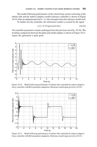
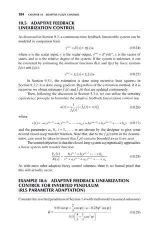
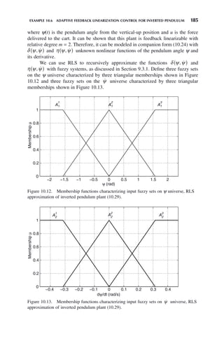
204. 186 CHAPTER 10 ADAPTIVE FUZZY CONTROL
The rule base of the fuzzy system approximating fδ is given by
1. If ψ is A1
1
and
ψ is A2
1
, then f̂δ
1
is a1
.
2. If ψ is A1
1
and
ψ is A2
2
, then f̂δ
2
is a2
.
3. If ψ is A1
1
and
ψ is A2
3
, then f̂δ
3
is a3
.
4. If ψ is A1
2
and
ψ is A2
1
, then f̂δ
4
is a4
.
5. If ψ is A1
2
and
ψ is A2
2
, then f̂δ
5
is a5
.
6. If ψ is A1
2
and
ψ is A2
3
, then f̂δ
6
is a6
.
7. If ψ is A1
3
and
ψ is A2
1
, then f̂δ
7
is a7
.
8. If ψ is A1
3
and
ψ is A2
2
, then f̂δ
8
is a8
.
9. If ψ is A1
3
and
ψ is A2
3
, then f̂δ
9
is a9
.
where ai
, i = 1, … , 9 are adjusted via RLS in this case. The crisp output, which is
an approximation of fδ, is
f̂ a
i
i
i
δ ξ
=
=
∑
1
9
(10.30)
where ξi is the fuzzy basis function for Rule i.
The rule base of the fuzzy system approximating fη is given by
1. If ψ is A1
1
and
ψ is A2
1
, then f̂η
1
is b1
.
2. If ψ is A1
1
and
ψ is A2
2
, then f̂η
2
is b2
.
3. If ψ is A1
1
and
ψ is A2
3
, then f̂η
3
is b3
.
4. If ψ is A1
2
and
ψ is A2
1
, then f̂η
4
is b4
.
5. If ψ is A1
2
and
ψ is A2
2
, then f̂η
5
is b5
.
6. If ψ is A1
2
and
ψ is A2
3
, then f̂η
6
is b6
.
7. If ψ is A1
3
and
ψ is A2
1
, then f̂η
7
is b7
.
8. If ψ is A1
3
and
ψ is A2
2
, then f̂η
8
is b8
.
9. If ψ is A1
3
and
ψ is A2
3
, then f̂η
9
is b9
.
where bi
, i = 1, … , 9 are adjusted via RLS. The crisp output, which is an approxi-
mation of fη, is
f̂ b
i
i
i
η ξ
=
=
∑
1
9
where ξi, i = 1, … , 9 are the same fuzzy basis functions as in (10.30) because the
rule premises are identical.
The resulting estimated plant in companion form is
y f f u a b u
i
i
i
i
i
i
T
≈ ( )+ ( ) = + =
= =
∑ ∑
ˆ , ˆ ,
δ η
ψ ψ ψ ψ ξ ξ φ θ
1
9
1
9
(10.31)
where
φ ξ ξ ξ ξ ξ ξ
T
u u u
= [ ]
1 2 9 1 2 9
θ = [ ]
a a a b b b
T
1 2 9 1 2 9

205. 10.6 SUMMARY 187
Since the estimated plant (10.31) is linear in the parameters θ, the unknown param-
eters ai
, bi
can be estimated via RLS (8.7) with the correction term equal to
ψ φ θ
k k k
T
( )− ( ) −
( )
[ ]
1 .
If we desire the rod angle to track the output of a linear system with transfer
function
Y s
R s
s
s s
m ( )
( )
=
+
+ +
64
16 64
2 (10.32)
excited by the reference signal
r t t
( ) = ( )
0 1 3
. sin π (10.33)
we apply the input
u t
f t
f t v t
( ) =
( )
− ( )+ ( )
( )
1
ˆ
ˆ
η
δ
with
v t t t r t r t
( ) = − ( )− ( )+ ( )+ ( )
16 64 64
ψ ψ
The resulting response is shown in Figure 10.14. In this figure, we see that the
rod angle tracks the reference model well.
Figure 10.14. Rod angle ψ(t) compared to model (10.32) output excited by reference
signal (10.33) under indirect adaptive feedback linearization control, RLS parameter
adaptation.
0 0.5 1 1.5 2 2.5 3
−0.2
−0.15
−0.1
−0.05
0
0.05
0.1
0.15
Time (s)
Rod
angle
(rad)
ym
ψ(t)
10.6 SUMMARY
This chapter shows how adaptive fuzzy controllers can be constructed. With the
methods discussed here it is possible to form tracking and model reference control-
lers for unknown nonlinear systems.

206. 188 CHAPTER 10 ADAPTIVE FUZZY CONTROL
Adaptive controllers are divided into two categories: direct and indirect. The
indirect adaptive control strategy involves identifying the plant and simultaneously
constructing a control law based on this identification. Thus the current estimate of
the plant model is used in the calculation of the control law. This is called the
certainty equivalence principle: the current plant model, even though incorrect, is
used in the calculation of the controller. The strategy is that over time the erroneous
controller converges to the correct controller as the identified plant approximation
converges to the correct plant model. The direct control approach directly calculates
the controller parameters without taking the extra step of identifying the plant.
For indirect adaptive control strategies in this book, we use either recursive
least squares or gradient parameter estimation, because these two methods are recur-
sive. We have discussed indirect adaptive tracking and model reference controllers
with the identified model in the form of a T–S fuzzy system with input–output dif-
ference equation consequents, although other forms of consequents are also possible.
We also discussed indirect adaptive feedback linearization in which the fuzzy model
is in Mamdani form. We have also given an example of direct adaptive fuzzy track-
ing control.
It should be kept in mind that there are no formal proofs of stability for any
of the methods presented in this chapter. Nevertheless, they have been used with
success in many applications.
EXERCISES
10.1 Find the characteristic polynomial of the matrix Λ in (10.2).
10.2 Repeat Example 10.1 with [k1 k2] = [3 2] and all other quantities the
same.
10.3 Simulate the direct adaptive controller designed in Example 10.1 with three
input fuzzy sets characterized by Gaussian membership functions on the x
and ẋ effective universes −
⎡
⎣
⎢
⎤
⎦
⎥
π π
2 2
, with the adjacent Gaussians crossing at
0.5 rather than the triangular membership functions of Figure 10.1. Verify
that your controller performs as desired.
10.4 The direct adaptive fuzzy model reference controller of Example 10.2 is
essentially an adaptive fuzzy tracking controller that forces the plant output
to track the output of the reference model. Discuss whether you think this
is a true model reference controller, or merely a tracking controller. Give
reasons for your conclusions.
10.5 (a) Is the reference signal r(t) of (10.16) periodic? Prove your answer.
(b) Is the gantry a minimum phase system? Explain.
10.6 In Example 10.2, assume that the model rules are of the form
Rip: If y(k) is Ai
1 and y(k − 1) is Ai
2, then
ˆ ˆ ˆ ˆ
y k a y k a y k b u k
i i i i
+
( ) = ( )+ −
( )+ ( )
1 1
1 2 1

207. EXERCISES 189
that is, u(k) is present in the consequent, but u(k − 1) is not.
(a) How many unknown parameters are there?
(b) Write the recursive least-squares parameter estimate laws to estimate
the unknown parameters.
(c) Write the rule in the controller fuzzy system that corresponds to Rule
ip above.
10.7 Show that the control laws 10.26 and 10.27 result in a linear closed-loop
system with transfer function given by 10.28.
10.8 Design an indirect adaptive fuzzy feedback linearization controller for the
motor-driven robotic link of Example 10.5. Let the closed-loop system be
linear with the transfer function
Y s
R s s s
m ( )
( )
=
+ +
10
4 10
2
10.9 Repeat Example 10.5 with three input fuzzy sets characterized by Gaussian
membership functions on the y(k) and y(k − 1) effective universes −
⎡
⎣
⎢
⎤
⎦
⎥
π π
2 2
,
with adjacent Gaussians crossing at 0.5 rather than the triangular member-
ship functions of Figure 10.9. Simulate and verify that your controller
performs as desired.
10.10 Repeat Example 10.6 using gradient parameter estimation rather than recur-
sive least squares. Simulate and verify that your controller performs as
desired. (Hint: You will probably have to use Gaussian input membership
functions rather than the triangular membership functions of Figs. 10.12
and 10.13).

208. 190
Fuzzy Control and Identification, By John H. Lilly
Copyright © 2010 John Wiley Sons, Inc.
1. Friedland, B., Advanced Control System Design, Prentice-Hall, Englewood Cliffs,
NJ, 1996.
2. Dorf, R. C. and Bishop, R. H., Modern Control Systems (10th ed.), Prentice-Hall,
Englewood Cliffs, NJ, 2005.
3. Franklin, G. F., Powell, J. D., Emami-Naeini, Feedback Control of Dynamic Systems
(5th ed.), Prentice Hall, Englewood Cliffs, NJ, 2006.
4. Ljung, L., System Identification: Theory for the User, Prentice-Hall, Englewood Cliffs
NJ, 1987.
5. Yager, R. R., Ovchinnikov, S., Tong, R. M. and Nguyen, H. T., Fuzzy Sets and Applications:
Selected Papers by L. A. Zadeh, John Wiley Sons, Inc., New York, 1987.
6. Zadeh, L. A., “Fuzzy Sets, Information and Control,” 8 (1965).
7. Mendel, J. M., Uncertain Rule-Based Fuzzy Logic Systems: Introduction and New
Directions, Prentice-Hall, Upper Saddle River, NJ, 2001.
8. Klir, G. J. and Yuan, B., Fuzzy Sets and Fuzzy Logic: Theory and Applications, Prentice-
Hall, Englewood Cliffs, NJ, 1995.
9. Passino, K. M. and Yurkovich, S., Fuzzy Control, Addison Wesley, 1998 (out of print).
Available at http://www.eleceng.ohio-state.edu/∼passino/FCbook.pdf
10. Ross, Timothy J., Fuzzy Logic with Engineering Applications, McGraw-Hill, New York,
1995.
11. Wang, L-X., A Course in Fuzzy Systems and Control, Prentice-Hall, Englewood Cliffs,
NJ, 1997.
12. Wang, L-X., Adaptive Fuzzy Systems and Control: Design and Stability Analysis,
Prentice-Hall, Englewood Cliffs, NJ, 1994.
13. Ying, Hao, Fuzzy Control and Modeling: Analytical Foundations and Applications, IEEE
Press, Piscataway, NJ, 2000.
14. Branson, J. S. and Lilly, J. H., “Incorporation, Characterization, and Conversion of
Negative Rules into Fuzzy Inference Systems,” IEEE Trans. Fuzzy Systems, 9(2) (April
2001).
15. Lilly, J. H., “Evolution of a Negative-rule Fuzzy Obstacle Avoidance Controller for an
Autonomous Vehicle,” IEEE Trans. Fuzzy Systems, 15(4) (Aug. 2007).
16. Chan, S. W., Lilly, J. H., Repperger, D. W. and Berlin, J. E. , “Fuzzy PD+I Learning
Control for a Pneumatic Muscle,” Proc. 2003 IEEE Int. Conf. on Fuzzy Systems (FUZZ-
IEEE’03), St. Louis, MO, May 2003.
17. Farinwata, S. S., Filev, D., Langari, R., Eds., Fuzzy Control: Synthesis and Analysis,
John WileySons, Inc., Chichester, England, 1999.
REFERENCES

209. REFERENCES 191
18. Mamdani, E., Adv. Linguistic Synth. Fuzzy Controllers, Int. J. Man-Machine Studies, 8(6)
(1976).
19. Close, C. M. and Frederick, D. K., Modeling and Analysis of Dynamic Systems, Houghton
Mifflin, Boston, 1978.
20. Chang, X. and Lilly, J. H., “Evolutionary Design of a Fuzzy Classifier from Data,” IEEE
Trans. Systems, Man, Cybernetics (Part B), 34(4) (Aug. 2004).
21. Vidyasagar, M., Nonlinear Systems Analysis (2nd ed.), Prentice-Hall, Englewood Cliffs,
NJ, 1993.
22. Khalil, H. K., Nonlinear Systems (2nd ed.), Prentice-Hall, Englewood Cliffs, NJ, 1996.
23. Brown, M. and Harris, C., Neurouzzy Adaptive Modelling and Control, Prentice-Hall,
New York, 1994.
24. de Silva, C. W., Intelligent Control: Fuzzy Logic Applications, CRC Press, Boca Raton,
FL, 1995.
25. Takagi, T. and Sugeno, M., “Fuzzy Identification of Systems and its Applications to
Modeling and Control,” IEEE Trans. Systems, Man, Cybernet., 15(1) (Jan. 1985).
26. Levine, William S., Ed., The Control Handbook, CRC Press, Boca Raton, FL, 1996.
27. Goodwin, G. C. and Sin, K. S., Adaptive Filtering, Prediction, and Control, Prentice-
Hall, Englewood Cliffs, NJ, 1984.
28. Wang, L-X. and Mendel, J. M., “Fuzzy Basis Functions, Universal Approximation, and
Orthogonal Least-squares Learning,” IEEE Trans. Neural Networks, 3(5) (Sept. 1992).
29. Tanaka, K. and Wang, H. O., Fuzzy Control Systems Design and Analysis: A Linear
Matrix Inequality Approach, John WileySons, Inc., New York, 2001.
30. Aracil, J. and Gordillo, F., Stability Issues in Fuzzy Control, Physica-Verlag, Heidelberg,
2000.
31. Boyd, S., El Ghaoui, L., Feron, E., and Balakrishnan, V., Linear Matrix Inequalities in
System and Control Theory, SIAM, Philadelphia, 1994.
32. Sorenson, Harold W., Parameter Estimation: Principles and Problems, Marcel Dekker,
New York, 1980.
33. Johnson, Jr., C. R., Lectures in Adaptive Parameter Estimation, Prentice-Hall, Englewood
Cliffs, NJ, 1988.
34. Luenberger, D. G., Linear and Nonlinear Programming, Addison-Wesley, Reading, MA,
1984.
35. Chang, X. and Lilly, J. H., “Fuzzy Control for Pneumatic Muscle Tracking via
Evolutionary Tuning,” Intell Automation Soft Comput, 9(4) (Sept. 2003).
36. Astrom, K. J. and Wittenmark, B., Computer Controlled Systems: Theory and Design
(3rd ed.), Prentice-Hall, Upper Saddle River, NJ, 1997.
37. Astrom, K. J. and Wittenmark, B., Adaptive Control (2nd ed.), Addison-Wesley, Reading,
MA, 1995.
38. Ioannou, P. A. and Sun, J., Robust Adaptive Control, Prentice-Hall, Upper Saddle River,
NJ, 1996.
39. Wellstead, P. E. and Zarrop, M. B., Self Tuning Systems, John Wiley Sons, Inc.,
Chichester, England, 1991.
40. Layne, J. R. and Passino, K. M., “Fuzzy Model Reference Learning Control,” J. Intel.
Fuzzy Systems, 4(1) (1996).

210. 192
Fuzzy Control and Identification, By John H. Lilly
Copyright © 2010 John Wiley Sons, Inc.
%tmfl evaluates left triangular membership function
%with corners m2 and m3 at point e
function tmfl=tmfl(e,m2,m3)
if e=m2
tmfl=1;
elseif em2 em3
tmfl=-(1/(m3-m2))*e+m3/(m3-m2);
else
tmfl=0;
end
%tmf evaluates triangular membership function
%with corners m1, m2, and m3 at point e
function tmf=tmf(e,m1,m2,m3)
if em1 e=m2
tmf=(1/(m2-m1))*e-m1/(m2-m1);
elseif em2 em3
tmf=-(1/(m3-m2))*e+m3/(m3-m2);
else
tmf=0;
end
%tmfr evaluates right triangular membership function
%with corners m1 and m2 at point e
function tmfr=tmfr(e,m1,m2)
if em1 e=m2
tmfr=(1/(m2-m1))*e-m1/(m2-m1);
elseif em2
tmfr=1;
COMPUTER PROGRAMS
APPENDIX

211. APPENDIX: COMPUTER PROGRAMS 193
else
tmfr=0;
end
%gmfl evaluates left gaussian membership function
%with center mid and spread sigma at point e
function gmfl=gmfl(e,mid,sigma)
if e=mid
gmfl=1;
else
gmfl=exp(-.5*((e-mid)/sigma)∧
2);
end
%gmf evaluates gaussian membership function
%with center mid and spread sigma at point e
function gmf=gmf(e,mid,sigma)
gmf=exp(-.5*((e-mid)/sigma)∧
2);
%gmfr evaluates right gaussian membership function
%with center mid and spread sigma at point e
function gmfr=gmfr(e, mid, sigma)
if emid
gmfr=1;
else
gmfr=exp(-.5*((e-mid)/sigma)∧
2);
end
%script fig2p1
%generates Figure 2.1
%single triangular mf
close all
clear all
T=-5:.01:40; %range of temperatures for plotting
for i=1:length(T)
mfT(i)=tmf(T(i),15,25,35);
end
plot(T,mfT,‘k’,‘linewidth’,2),grid
axis([-5 40 0 1.2]);

212. 194 APPENDIX: COMPUTER PROGRAMS
%script fig2p2
%generates Figure 2.2
%single gaussian mf
close all
clear all
T=-5:.01:40; %range of temperatures for plotting
for i=1:length(T)
mfT(i)=gmf(T(i),25,5);
end
plot(T,mfT,‘k’,‘linewidth’,2),grid
axis([-5 40 0 1.2]);
%script fig2p3
%generates figure 2.3
%illogical mf
T=-5:.1:40; %range of temperatures for plotting
for i=1:length(T)
if T(i)20
mu(i)=exp(-.5*((T(i)-20)/5)∧
2);
elseif t(i)=30
mu(i)=exp(-.5*((T(i)-30)/5)∧
2);
elseif t(i)=20 T(i)30
mu(i)=.5*(1.5+.5*cos(.1*2*pi*(T(i)-20)));
end
end
plot(T,mu,‘k’,‘linewidth’,2),grid
axis([-5 40 0 1.2])
%script fig2p4
%generates figure 2.4
%asymmetrical gaussian mf
close all
clear all
T=-5:.1:40; %range of temperatures for plotting
for i=1:length(T)
if T(i)25
mu(i)=gmf(T(i),25,7);

213. APPENDIX: COMPUTER PROGRAMS 195
elseif T(i)=25
mu(i)=gmf(T(i),25,3);
end
end
plot(T,mu,‘k’,‘linewidth’,2),grid
axis([-5 40 0 1.2])
%script fig2p5
%generates Figure 2.5
%4 gaussian mfs
close all
clear all
T=linspace(-10,45,500); %range of temperatures for plotting
center=[5 15 25 35]; %centers of memberships
%spread for adjacent mfs crossing at .6
sigma=.5*(center(2)-center(1))/sqrt(-2*log(.6));
for i=1:length(T)
gmf1(i)=gmfl(T(i),center(1),sigma);
gmf2(i)=gmf(T(i),center(2),sigma);
gmf3(i)=gmf(T(i),center(3),sigma);
gmf4(i)=gmfr(T(i),center(4),sigma);
end
plot(T,gmf1,‘k’,T,gmf2,‘k’,T,gmf3,‘k’,T,gmf4,‘k’,…‘linewidth’,
2),grid;
axis([-10 45 0 1.2])
%fig2p12
%generates figure 2.12
%Cartesian product of 2 fuzzy sets
close all
clear all
S=0:1:50; %range of wind speeds for plotting
T=-10:1:40; %range of temperatures for plotting
for i=1:length(T)
for j=1:length(S)
mu(i,j)=gmf(T(i),25,5)*gmf(S(j),15,4);
end
end
colormap(white)
surface(T,S,mu’),view(43,15),grid

214. 196 APPENDIX: COMPUTER PROGRAMS
%script fig3p2
%generates Figure 3.2
%4 triangular mfs
close all
clear all
center=[0 10 20 30]; %membership centers
Temp=-5:.1:35; %range of temperatures for plotting
for i=1:length(Temp)
COLD(i)=tmfl(Temp(i),center(1),center(2));
COOL(i)=tmf(Temp(i),center(1),center(2),center(3));
WARM(i)=tmf(Temp(i),center(2),center(3),center(4));
HOT(i)=tmfr(Temp(i),center(3),center(4));
end
plot(Temp,COLD,‘k’,Temp,COOL,‘k’,Temp,WARM,‘k’,…
Temp,HOT,‘k’,‘linewidth’,2),grid
axis([-5 35 0 1.2])
%script fig3p6
%generates Figure 3.6 using min T-norm and COG
%defuzzification
%windchill input-output characteristic
close all; %close all open plots
clear all; %clear all variables in the work space
numpts=50; %number of values of temp and
%windspeed at which to evaluate mfs
midT=[0 10 20 30]; %mid points of mfs on temp ud
midS=[5 15 25]; %mid points of mfs on windspeed ud
midW=[-25 -10 5 20 35]; %mid points of mfs on windchill ud
w=midW(3)-midW(1); %widths of bases of windchill triangles
%centers of area of output mfs
FRIG=midW(1);
COLD=midW(2);
COOL=midW(3);
COMF=midW(4);
WARM=midW(5);
%rule base
rule=[COOL COLD FRIG;…
COMF COOL COLD;…
WARM COMF COOL;…
WARM WARM COMF];

215. APPENDIX: COMPUTER PROGRAMS 197
%define numpts points equally spaced T and S uds
T=linspace(-5,35,numpts);
S=linspace(0,30,numpts);
%for each of the numpts∧
2 points defined in temp x windspeed
%plane, calculate the corresponding wind chill
for i=1:numpts
for j=1:numpts
%calculate degree of membership in the 4 temp fuzzy sets
mfT=[tmfl(T(i),midT(1),midT(2))…
tmf(T(i),midT(1),midT(2),midT(3))…
tmf(T(i),midT(2),midT(3),midT(4))
tmfr(T(i),midT(3),midT(4))];
%calculate degree of membership in the 3 windspeed fuzzy
%sets
mfS=[tmfl(S(j),midS(1),17.5)…
tmf(S(j),2.5,midS(2),27.5)…
tmfr(S(j),12.5,midS(3))];
%calculate the degree of firing of each of the 12 rules
%using min T-norm. prem is a 4x3 matrix
for k=1:4
for l=1:3
prem(k,l)=min(mfT(k),mfS(l));
end
end
%the heights of the implied fuzzy sets (trapezoids)
%h is a 4x3 matrix
h=prem;
%the areas of the implied fuzzy sets (trapezoids)
%h is a 4x3 matrix
areaimp=w*(h-h.∧
2/2);
num=sum(sum(areaimp.*rule));
den=sum(sum(areaimp));
%the crisp output (windchill) corresponding to the
%ith value of temperature and the jth value of windspeed
windchill(i,j)=num/den;
end
end

216. 198 APPENDIX: COMPUTER PROGRAMS
axis([-5 35 0 30 -30 40]);
colormap(white)
surface(T,S,windchill’),view(200,15),grid
xlabel(‘Temperature’)
ylabel(‘Wind speed’)
zlabel(‘Windchill’)
%script fig4p12
%generates Figure 4.12, product T-norm, CA defuzzification
%states: x(1)=x, x(2)=xdot
%4th order Runge-Kutta integration
%response of ball and beam under fuzzy control
close all
clear all
%g0=1; %scaling gain
%g1=1; %scaling gain
%h=1; %scaling gain
%g0=1; %scaling gain
%g1=18; %scaling gain
%h=1; %scaling gain
g0=3; %scaling gain
g1=18; %scaling gain
h=1; %scaling gain
%g0=3; %scaling gain
%g1=18; %scaling gain
%h=7; %scaling gain
X1=[]; %placeholder for X1 array
V=[]; %placeholder for V array
T=[]; %placeholder for T array
x=[-.4 0]; %initial conditions
dx=[0 0];
t=0; %initial time
dt=.001; %time step
tfinal=10-dt; %final time
k=.01; %motor shaft angle-to-voltage ratio
g=9.81; %acceleration of gravity (m/s∧
2)
%triangle midpoints on e, c, and F universes
mid=[-1 -.5 0 .5 1];
mide=.5*mid; %triangle mid-points on e universe
midc=4*mid; %triangle mid-points on c universe
midv=10*mid; %triangle mid-points on v universe
base=midv(3)-midv(1); %base of output triangles

217. APPENDIX: COMPUTER PROGRAMS 199
%locations of output singletons
NL=midv(1);
NS=midv(2);
ZE=midv(3);
PS=midv(4);
PL=midv(5);
%rule base
rule=[NL NL NL NS ZE; …
NL NL NS ZE PS; …
NL NS ZE PS PL; …
NS ZE PS PL PL; …
ZE PS PL PL PL];
while t=tfinal
x1previous=x(1); %needed to approximate dx/dt
for n=1:4 %needed for RK4 algorithm
%inputs to fuzzy controller
e=-x(1);
c=-(x(1)-x1previous)/dt; %approximation of dx/dt
%membership function values corresponding to e above
mfe=[tmfl(g0*e,mide(1),mide(2))…
tmf(g0*e,mide(1),mide(2),mide(3))…
tmf(g0*e,mide(2),mide(3),mide(4))…
tmf(g0*e,mide(3),mide(4),mide(5))…
tmfr(g0*e,mide(4),mide(5))];
%membership function values corresponding to c above
mfc=[tmfl(g1*c,midc(1),midc(2))…
tmf(g1*c,midc(1),midc(2),midc(3))…
tmf(g1*c,midc(2),midc(3),midc(4))…
tmf(g1*c,midc(3),midc(4),midc(5))…
tmfr(g1*c,midc(4),midc(5))];
%calculate degrees of firing of all rules
prem=mfe′*mfc;
%calculate crisp output via CA defuzzification
num=sum(sum(rule.*prem));
den=sum(sum(prem));
volts=h*num/den; %crisp output
% ball and beam model
dx(1)=x(2);
dx(2)=g*sin(k*volts);

218. 200 APPENDIX: COMPUTER PROGRAMS
%RK4 generic code between dotted lines
%-------------------------------------------------------------
if n==1
z=dx;
v=x;
x=v+0.5*dt*dx;
t=t+0.5*dt;
elseif n==2
z=z+2*dx;
x=v+0.5*dt*dx;
elseif n==3
z=z+2*dx;
x=v+dt*dx;
t=t+0.5*dt;
elseif n==4
x=v+(dt/6)*(z+dx);
end
%-------------------------------------------------------------
end
X1=[X1 x(1)]; %save current state x(1) for plotting
V=[V volts]; %save current input (V) for plotting
T=[T t];
end
plot(T,X1,‘k’,‘linewidth’,2),grid
%script fig4p18
%generates Figure 4.18
%Gaussian input memberships, product T-norm
%input–output characteristic of fuzzy controller for
%ball and beam
close all; %close all open plots
clear all; %clear all variables in the work space
numpts=40; %number of values of e and edot at which to
%evaluate mfs
mids=[-1 -.5 0 .5 1]; %gaussian midpoints on error universe
mide=.5*mids;
midc=4*mids;
midf=10*mids;
%spreads for adjacent mfs crossing at .5
sigmae=.5*(mide(2)-mide(1))/sqrt(-2*log(.5));
sigmac=.5*(midc(2)-midc(1))/sqrt(-2*log(.5));

219. APPENDIX: COMPUTER PROGRAMS 201
%linguistic values for output mfs
NL=midf(1);
NS=midf(2);
ZE=midf(3);
PS=midf(4);
PL=midf(5);
%rule base
rule=[NL NL NL NS ZE; …
NL NL NS ZE PS; …
NL NS ZE PS PL; …
NS ZE PS PL PL; …
ZE PS PL PL PL];
%define numpts points equally spaced e and c uds
e=linspace(-.55,.55,numpts);
c=linspace(-4.4,4.4,numpts);
for i=1:numpts
for j=1:numpts
%membership function values corresponding to e above
mfe=[gmfl(e(i),mide(1),sigmae) …
gmf(e(i),mide(2),sigmae) …
gmf(e(i),mide(3),sigmae) …
gmf(e(i),mide(4),sigmae) …
gmfr(e(i),mide(5),sigmae)];
%membership function values corresponding to c above
mfc=[gmfl(c(j),midc(1),sigmac) …
gmf(c(j),midc(2),sigmac) …
gmf(c(j),midc(3),sigmac) …
gmf(c(j),midc(4),sigmac) …
gmfr(c(j),midc(5),sigmac)];
prem=mfe′*mfc; %degrees of firing of all rules
%calculate crisp output
num=sum(sum(rule.*prem));
den=sum(sum(prem));
ufuzzy(i,j)=num/den;
end
end
axis([-0.55 0.55 -4.4 4.4 -12 12]);
colormap(white)
surface(e,c,ufuzzy’),view(20,15),grid

220. 202 APPENDIX: COMPUTER PROGRAMS
%script fig4p26
%generates Figure 4.26
%input–output characteristics of
%PD and fuzzy controllers for inverted pendulum
close all; %close all open plots
clear all; %clear all variables in the work space
numpts=20; %number of values of e and edot at which to
%evaluate mfs
P=30; %proportional gain
D=5; %derivative gain
maxf=3; %max control effort resulting from pd with above P
%and D gains
mids5=[-1 -.5 0 .5 1];
mids9=[-2 -1.5 mids5 1.5 2];
mide=(2*maxf/P)*mids5; %triangle mid-points on e universe
midc=(2*maxf/D)*mids5; %triangle mid-points on c universe
midf=2*maxf*mids9; %unredesigned singleton locations on
%F universe
%redesigned singleton locations on F universe
NLLL=2.5*midf(1);
NLL=2*midf(2);
NL=1.5*midf(3);
NS=midf(4);
ZE=midf(5);
PS=midf(6);
PL=1.5*midf(7);
PLL=2*midf(8);
PLLL=2.5*midf(9);
%generic rule base for equivalent fuzzy PD controller
rule=[NLLL NLL NL NS ZE; …
NLL NL NS ZE PS; …
NL NS ZE PS PL; …
NS ZE PS PL PLL; …
ZE PS PL PLL PLLL];
%define numpts equally spaced points on e and c universes
e=linspace(-.2,.2,numpts);
c=linspace(-1.2,1.2,numpts);
for i=1:numpts
for j=1:numpts

221. APPENDIX: COMPUTER PROGRAMS 203
%membership function values corresponding to e above
mfe=[tmfl(e(i),mide(1),mide(2)) …
tmf(e(i),mide(1),mide(2),mide(3)) …
tmf(e(i),mide(2),mide(3),mide(4)) …
tmf(e(i),mide(3),mide(4),mide(5)) …
tmfr(e(i),mide(4),mide(5))];
%membership function values corresponding to c above
mfc=[tmfl(c(j),midc(1),midc(2)) …
tmf(c(j),midc(1),midc(2),midc(3)) …
tmf(c(j),midc(2),midc(3),midc(4)) …
tmf(c(j),midc(3),midc(4),midc(5)) …
tmfr(c(j),midc(4),midc(5))];
prem=mfe′*mfc; %degree of firing of all rules
%crisp output of nonlinear fuzzy controller
num=sum(sum(rule.*prem));
den=sum(sum(prem));
ufuzzy(i,j)=-num/den;
%output of nonfuzzy PD controller
upid(i,j)=-(P*e(i)+D*c(j));
end
end
hold on
axis(1.1*[-0.2 0.2 -1.2 1.2 -30 30]);
colormap(white)
surface(e,c,ufuzzy’)
surface(e,c,upid’),view(200,10),grid
%script Ex5p1
%Example 5.1 - Plots output of forced pendulum, nonlinear
%differential equation model
close all
clear all
M=1; %pendulum mass (kg)
l=1; %1/2 of pendulum length (m)
I=M*l∧
2; %moment of inertia of pendulum
B=1; %coefficient of friction at attach point
g=9.81; %acceleration of gravity (m/sec∧
2)
X1=[]; %placeholder for x(1) array
X2=[];
U=[];
T=[];

222. 204 APPENDIX: COMPUTER PROGRAMS
t=0; %initial time
dt=.001; %step size for RK4 routine
x=[0;0]; %initial conditions
dx=[0;0];
final time=10-dt;
while tfinaltime
for n=1:4 %part of generic RK4 code
%specification of input
if t=2
u=2*sin(2*pi*t);
else
u=0;
end
%mathematical model of forced pendulum
dx(1)=x(2);
dx(2)=(-B*x(2)-M*g*l*sin(x(1))+u)/I;
%generic RK4 code between dotted lines
%-------------------------------------------------------------
if n==1
z=dx;
v=x;
x=v+0.5*dt*dx;
t=t+0.5*dt;
elseif n==2
z=z+2*dx;
x=v+0.5*dt*dx;
elseif n==3
z=z+2*dx;
x=v+dt*dx;
t=t+0.5*dt;
elseif n==4
x=v+(dt/6)*(z+dx);
end
%-------------------------------------------------------------
end
X1=[X1 x(1)]; %save for plotting
X2=[X2 x(2)];
U=[U u];
T=[T t];

223. APPENDIX: COMPUTER PROGRAMS 205
end
plot(T,X1,‘k’,‘linewidth’,2),grid
%script Ex5p3
%Example 5.3 - Plots output of forced pendulum,
%discrete-time state equation model
t=0:.01:10; %sample times
x1=0; %initial condition
x2=0; %initial condition
X1=[]; %used for plotting
for k=1:length(t)
%input torque to pendulum
if t(k)=2
u=2*sin(2*pi*t(k));
else
u=0;
end
%discrete state equation model of pendulum
x1n=x1+.01*x2;
x2n=-.098*x1+.99*x2+.01*u;
%update states for next iteration
x1=x1n;
x2=x2n;
%save x1 values for plotting
X1=[X1 x1];
end
plot(t,X1(1:length(t)),‘k’,‘linewidth’,3),grid
%script Ex5p4
%Example 5.4 - Plots output of forced pendulum, linear
%input–output %difference equation model
dt=.01;
t=0:dt:10; %sample times
ykm1=0; %initial value of y(k-1)
ykm2=0; %initial value of y(k-2)
Y=[]; %placeholder for y(k) array
for k=1:length(t)
if t(k)=0+2*dt t(k)=2+2*dt
ukm2=2*sin(2*pi*t(k-2));

224. 206 APPENDIX: COMPUTER PROGRAMS
else
ukm2=0;
end
%input-output difference equation
yk=1.99*ykm1-.991*ykm2+.0001*ukm2;
ykm2=ykm1; %when time advances, y(k-1) becomes y(k-2)
ykm1=yk; %when time advances, y(k) becomes y(k-1)
Y=[Y yk]; %save values of y(k) for plotting
end
plot(t,Y,‘k’,‘linewidth’,3),grid
%script fig6p6
%creates Figure 6.6
%plots the states of a T-S fuzzy system that interpolates
%four time-invariant continuous-time linear systems
close all
clear all
%corners of triangle mfs on x1 and x2 uds
midx1=[-1 1];
midx2=[-2 2];
%coefficients in consequents of TS fuzzy rules
A1=[0 1;-2 -2];
A2=[0 1;-1 -2];
A3=[0 1;-3 -2];
A4=[1 1;-2 -2];
b1=[0;2];
b2=[2;2];
b3=[-2;2];
b4=[0;-2];
x=[0;0]; %initial conditions of state
dx=[0;0]; %initial conditions of derivatives of states
%placeholders for plotting saved variables
X1=[];
X2=[];
T=[];
t=0; %initial time
dt=.01; %step size of RK4 routine
finaltime=10-dt;
while tfinaltime

225. APPENDIX: COMPUTER PROGRAMS 207
for n=1:4 %part of RK4 routine
u=3*sin(pi*t); %input
%individual mf values corresponding to current x1 and x2
mux1=[tmfl(x(1),midx1(1),midx1(2)) …
tmfr(x(1),midx1(1),midx1(2))];
mux2=[tmfl(x(2),midx2(1),midx2(2)) …
tmfr(x(2),midx2(1),midx2(2))];
%degrees of firing of all rules, product T-norm
mu=mux1′*mux2;
%fuzzy basis functions
zeta=mu/sum(sum(mu));
%overall A and b corresponding to current x1, x2
A=zeta(1,1)*A1+zeta(1,2)*A2+…
zeta(2,1)*A3+zeta(2,2)*A4;
b=(zeta(1,1)*b1+zeta(1,2)*b2+…
zeta(2,1)*b3+zeta(2,2)*b4);
%overall DE
dx=A*x+b*u;
%RK4 algorithm between dotted lines----------------
if n==1
z=dx;
v=x;
x=v+0.5*dt*dx;
t=t+0.5*dt;
elseif n==2
z=z+2*dx;
x=v+0.5*dt*dx;
elseif n==3
z=z+2*dx;
x=v+dt*dx;
t=t+0.5*dt;
elseif n==4
x=v+(dt/6)*(z+dx);
end
%-------------------------------------------------------------
end
X1=[X1 x(1)];
X2=[X2 x(2)];
T=[T t];

226. 208 APPENDIX: COMPUTER PROGRAMS
end
plot(T,X1,T,X2,‘linewidth’,2),grid
xlabel(‘Time (seconds)’)
ylabel(‘States’)
%script fig6p7
%creates Figure 6.7
%plots the states of a T-S fuzzy system that interpolates
%four time-invariant discrete-time linear systems
close all
clear all
dt=.2; %sample time
finaltime=9;
t=0:dt:finaltime; %times at which to calculate the states
%corners of triangle mfs on x1 and x2 uds
midx=[-1 1];
%coefficients in consequents of TS fuzzy rules
A1=[0.1 0;-0.2 0.2];
A2=[0 0.1;1 -0.2];
A3=[-0.3 1;0 0.2];
A4=[0.1 1;0.2 0.5];
b1=[0;1];
b2=[0.1;1];
b3=[-0.1;1];
b4=[0;-1];
x=[0;0]; %initial conditions of state
%placeholders for plotting saved variables
X1=[];
X2=[];
U=[];
for k=1:length(t)
%individual mf values corresponding to current x1 and x2
mux1=[tmfl(x(1),midx(1),midx(2)) …
tmfr(x(1),midx(1),midx(2))];
mux2=[tmfl(x(2),midx(1),midx(2)) …
tmfr(x(2),midx(1),midx(2))];
%degrees of firing of all rules, product T-norm
mu=mux1′*mux2;
%fuzzy basis functions
zeta=mu/sum(sum(mu));

227. APPENDIX: COMPUTER PROGRAMS 209
%overall A and b corresponding to current x1, x2
A=(zeta(1,1)*A1+zeta(1,2)*A2+zeta(2,1)*A3+zeta(2,2)*A4);
b=(zeta(1,1)*b1+zeta(1,2)*b2+zeta(2,1)*b3+zeta(2,2)*b4);
u=sin(.5*pi*t(k)); %new u(k)
%overall difference equation
x=A*x+b*u;
X1=[X1 x(1)];
X2=[X2 x(2)];
U=[U u];
end
plot(t,X1,‘o’,t,X2,‘o’,t,U,‘s’),grid
legend(‘x1(t)’,‘x2(t)’,‘u(t)’);
xlabel(‘Time (seconds)’)
ylabel(‘States’)
axis([0 9 -1.2 1.2])
%script fig6p8
%creates Figure 6.8
%time-varying discrete system in input–output difference
%equation form from a four-rule TS fuzzy system
close all
clear all
dt=1; %sample time
finaltime=60;
t=0:dt:finaltime; %times at which to calculate the states
%corners of Gaussian mfs on y(k) and y(k-1) uds
midy=[-1 1];
%spread for adjacent Gaussians crossing at 0.5
sigma=.5*(midy(2)-midy(1))/sqrt(-2*log(.5));
ukm1=0; %initial u(k-1)
uk=0; %initial u(k)
ykm1=0; %initial y(k-1)
yk=0; %initial y(k)
%placeholders for y and u arrays
Y=[];
U=[];
%coefficients of y(k) in rule consequents
param1=[.5 .4 .2 .8];

228. 210 APPENDIX: COMPUTER PROGRAMS
%coefficients of y(k-1) in rule consequents
param2=[-.5 -.8 .5 -.6];
%coefficients of u(k) in rule consequents
param3=[1 1.2 1.5 -1.5];
%coefficients of u(k-1) in rule consequents
param4=[.6 -1 -.7 1];
for k=1:length(t)
%calculate degrees of membership in all input fuzzy sets
muyk=[gmfl(yk,midy(1),sigma) …
gmfr(yk,midy(2),sigma)];
muykm1=[gmfl(ykm1,midy(1),sigma) …
gmfr(ykm1,midy(2),sigma)];
%calculate degrees of firing of all rules
mu=muyk′*muykm1;
%calculate fuzzy basis functions
zeta=[mu(1,:)/sum(sum(mu)) mu(2,:)/sum(sum(mu))];
%calculate y(k+1)
ykp1=(param1*zeta’)*yk+(param2*zeta’)*ykm1+…
(param3*zeta’)*uk+(param4*zeta’)*ukm1;
%update y(k-1), y(k), u(k-1), u(k)
ykm1=yk;
yk=ykp1;
ukm1=uk;
uk=sin(.05*pi*t(k));
%save y(k) and u(k) for plotting
Y=[Y yk];
U=[U uk];
end
hold on
plot(t,U,’s’,‘linewidth’,2,‘color’,[.7.7.7])
plot(t,Y,‘o’,‘linewidth’,2,‘color’,‘k’),grid
legend(‘itu(t)’,‘ity(t)’,‘Location’,’Southwest’);
xlabel(‘Time (seconds)’)
ylabel(‘States’)
axis([0 60 -2 1.2])
%script ex7p1
%parallel distributed pole placement for a CT nonlinear
%system
close all
clear all

229. APPENDIX: COMPUTER PROGRAMS 211
%corners of saturated Gaussian mfs on x1, x2 uds
mid=[-1 1];
cross=0.5; %crossing point of adjacent mfs
%spread for adjacent mfs crossing at 0.5
sigma=.5*(mid(2)-mid(1))/sqrt(-2*log(cross));
%coefficients in consequents of plant TS fuzzy rules
A1=[0 1;-2 2];
A2=[0 1;-3 2];
A3=[0 1;-2 1];
A4=[0 1;-3 1];
b1=[0;1];
b2=[0;1];
b3=[0;1];
b4=[0;1];
%coefficients in consequents of controller TS fuzzy
rules k1=[0 4];
k2=[-1 4];
k3=[0 3];
k4=[-1 3];
x=[1;-1]; %initial condition of state
dx=[0;0]; %initial condition of derivative of state
X1=[];
X2=[];
U=[];
T=[];
t=0; %initial time
dt=0.01; %step size of RK4 routine
finaltime=6-dt;
while tfinaltime
for n=1:4 %part of RK4 routine
%degrees of belongingness in fuzzy sets on x1, x2 universes
mu11=gmfl(x(1),mid(1),sigma);
mu12=gmfr(x(1),mid(2),sigma);
mu21=gmfl(x(2),mid(1),sigma);
mu22=gmfr(x(2),mid(2),sigma);
%degrees of firing of rules
mu1=mu11*mu21;
mu2=mu11*mu22;
mu3=mu12*mu21;
mu4=mu12*mu22;

230. 212 APPENDIX: COMPUTER PROGRAMS
%fuzzy basis functions
zeta1=mu1/(mu1+mu2+mu3+mu4);
zeta2=mu2/(mu1+mu2+mu3+mu4);
zeta3=mu3/(mu1+mu2+mu3+mu4);
zeta4=mu4/(mu1+mu2+mu3+mu4);
%overall A, b, and k
A=(zeta1*A1+zeta2*A2+zeta3*A3+zeta4*A4);
b=(zeta1*b1+zeta2*b2+zeta3*b3+zeta4*b4);
k=(zeta1*k1+zeta2*k2+zeta3*k3+zeta4*k4);
%feedback control law
u=-k*x;
%closed-loop system
dx=A*x+b*u;
%RK4 routine from here to dotted line
if n==1
z=dx;
v=x;
x=v+0.5*dt*dx;
t=t+0.5*dt;
elseif n==2
z=z+2*dx;
x=v+0.5*dt*dx;
elseif n==3
z=z+2*dx;
x=v+dt*dx;
t=t+0.5*dt;
elseif n==4
x=v+(dt/6)*(z+dx);
end
%-------------------------------------------------------------
end
%save variables for plotting
X1=[X1 x(1)];
X2=[X2 x(2)];
U=[U u];
T=[T t];
end
plot(T,X1,‘k’,T,X2,‘k’,‘linewidth’,3),grid

231. APPENDIX: COMPUTER PROGRAMS 213
%script ex7p2
%parallel distributed pole placement for a DT nonlinear
%system
close all
clear all
%corners of saturated Gaussian mfs on x1, x2 uds
mid=[-1 1];
cross=0.5; %crossing point of adjacent mfs
%spread for adjacent mfs crossing at cross
sigma=.5*(mid(2)-mid(1))/sqrt(-2*log(cross));
%matrices in consequents of plant TS fuzzy rules
A1=[0 1;-1 1];
A2=[1 1;-1 2];
A3=[0 1;-.2 1];
A4=[1 1;-.3 1];
b1=[0;1];
b2=[0;1];
b3=[0;1];
b4=[0;1];
%feedback gains in consequents of controller TS fuzzy rules
k1=[-1.25 1];
k2=[-0.25 3];
k3=[-0.45 1];
k4=[0.45 2];
x=[1;-1]; %initial condition of state
%placeholders for plotting states
X1=[];
X2=[];
U=[];
T=[];
t=0;
dt=0.1; %sample time
finaltime=1;
while tfinaltime
%degrees of belongingness in fuzzy sets on x1, x2 universes
mu11=gmfl(x(1),mid(1),sigma);
mu12=gmfr(x(1),mid(2),sigma);
mu21=gmfl(x(2),mid(1),sigma);
mu22=gmfr(x(2),mid(2),sigma);

232. 214 APPENDIX: COMPUTER PROGRAMS
%degrees of firing of rules
mu1=mu11*mu21;
mu2=mu11*mu22;
mu3=mu12*mu21;
mu4=mu12*mu22;
%fuzzy basis functions
zeta1=mu1/(mu1+mu2+mu3+mu4);
zeta2=mu2/(mu1+mu2+mu3+mu4);
zeta3=mu3/(mu1+mu2+mu3+mu4);
zeta4=mu4/(mu1+mu2+mu3+mu4);
%overall A, b, and k
A=(zeta1*A1+zeta2*A2+zeta3*A3+zeta4*A4);
b=(zeta1*b1+zeta2*b2+zeta3*b3+zeta4*b4);
k=(zeta1*k1+zeta2*k2+zeta3*k3+zeta4*k4);
%feedback control law
u=-k*x;
%closed-loop system
%save variables for plotting
X1=[X1 x(1)];
X2=[X2 x(2)];
U=[U u];
T=[T t];
t=t+dt;
x=A*x+b*u; %nonlinear system model
end
hold on
plot(T,X1,‘ko’,T,X2,‘ko’,‘markersize’,10,‘linewidth’,3),grid
legend(‘itx1(t)’,‘itx2(t)’)
axis([0 1 -1.2 1.2])
%script ex7p3
%Example 7.3, parallel distributed one-step-ahead tracking
close all
clear all
finaltime=20;
k=0; %initial time
%corners of triangle mfs on y(k) and y(k-1) uds
midy=[-1 1];

233. APPENDIX: COMPUTER PROGRAMS 215
ukm1=0; %initial u(k-1)=u(-1)
uk=0; %initial u(k)=u(0)
ykm1=-1; %initial y(k-1)=y(-1)
yk=1; %initial y(k)=y(0)
%placeholders for vectors saved for plotting
Y=[];
R=[];
K=[];
while k=finaltime
%evaluate memberships for present y(k), y(k-1)
mu11=tmfl(yk,midy(1),midy(2));
mu12=tmfr(yk,midy(1),midy(2));
mu21=tmfl(ykm1,midy(1),midy(2));
mu22=tmfr(ykm1,midy(1),midy(2));
%calculate degrees of firing of all rules
mu1=mu11*mu21;
mu2=mu11*mu22;
mu3=mu12*mu21;
mu4=mu12*mu22;
%calculate basis functions
zeta1=mu1/(mu1+mu2+mu3+mu4);
zeta2=mu2/(mu1+mu2+mu3+mu4);
zeta3=mu3/(mu1+mu2+mu3+mu4);
zeta4=mu4/(mu1+mu2+mu3+mu4);
%calculate one-step-ahead reference signal to be tracked
rk=0.5*sin(0.2*pi*k);
rkp1=0.5*sin(0.2*pi*(k+1));
%calculate consequents of controller fuzzy system
ccons1=-0.6*ukm1-1.5*yk+0.4*ykm1+rkp1;
ccons2=(-ukm1-0.4*yk+1.8*ykm1+rkp1)/1.2;
ccons3=(-0.7*ukm1-1.2*yk-0.5*ykm1+rkp1)/1.5;
ccons4=(-ukm1-0.8*yk+1.6*ykm1+rkp1)/1.5;
%calculate control signal u(k)
uk=zeta1*ccons1+zeta2*ccons2+zeta3*ccons3+zeta4*ccons4;
%calculate consequents of plant fuzzy system
pcons1=1.5*yk-0.4*ykm1+uk+0.6*ukm1;
pcons2=0.4*yk-1.8*ykm1+1.2*uk+ukm1;
pcons3=1.2*yk+0.5*ykm1+1.5*uk+0.7*ukm1;
pcons4=0.8*yk-1.6*ykm1+1.5*uk+ukm1;
%calculate y(k+1) of plant fuzzy system

234. 216 APPENDIX: COMPUTER PROGRAMS
ykp1=zeta1*pcons1+zeta2*pcons2+…
zeta3*pcons3+zeta4*pcons4;
%save y(k) and r(k) for plotting
Y=[Y yk];
R=[R rk];
K=[K k];
%update u and y for next iteration
ukm1=uk;
ykm1=yk;
yk=ykp1;
k=k+1;
end
%plot tracking error
%plot(K,Y,‘ko’,K,R,‘ksq’),gridplot(K,Y,‘ko’,K,R,‘ksq’,
‘markersize’,10,‘linewidth’,3),grid
%plot(K,Y-R,‘ko’,‘markersize’,10,‘linewidth’,3),grid
legend(‘ity(t)’,‘itr(t)’)
axis([0 20 -0.6 1.2])
%script ex7p4
%Example 7.4, parallel distributed model reference control
close all
clear all
finaltime=20;
k=0; %initial time
%corners of saturated triangle mfs on y(k) and y(k-1) uds
midy=[-1 1];
ukm1=0; %initial plant input u(k-1)=u(-1)
uk=0; %initial plant input u(k)=u(0)
ykm1=-1; %initial plant output y(k-1)=y(-1)
yk=1; %initial plant output y(k)=y(0)
Ykm1=0; %initial reference model output Y(k-1)
Yk=0; %initial reference model output Y(k)
rk=0; %initial reference model input r(k)
%placeholders for vectors saved for plotting
Y=[];
YM=[];
K=[];
while k=finaltime

235. APPENDIX: COMPUTER PROGRAMS 217
%evaluate memberships for present y(k), y(k-1)
mu11=tmfl(yk,midy(1),midy(2));
mu12=tmfr(yk,midy(1),midy(2));
mu21=tmfl(ykm1,midy(1),midy(2));
mu22=tmfr(ykm1,midy(1),midy(2));
%calculate degrees of firing of all rules
mu1=mu11*mu21;
mu2=mu11*mu22;
mu3=mu12*mu21;
mu4=mu12*mu22;
%calculate basis functions
zeta1=mu1/(mu1+mu2+mu3+mu4);
zeta2=mu2/(mu1+mu2+mu3+mu4);
zeta3=mu3/(mu1+mu2+mu3+mu4);
zeta4=mu4/(mu1+mu2+mu3+mu4);
%calculate reference input
rkm1=rk;
rk=0.5*sin(0.2*pi*k);
%calculate reference model output
Ykp1=-0.5*Yk-0.5*Ykm1+2*rk+0.6*rkm1;
%calculate consequents of controller fuzzy system
ccons1=-0.6*ukm1-2*yk-0.1*ykm1+2*rk+0.6*rkm1;
ccons2=(-ukm1-0.9*yk+1.3*ykm1+2*rk+0.6*rkm1)/1.2;
ccons3=(-0.7*ukm1-1.7*yk-ykm1+2*rk+0.6*rkm1)/1.5;
ccons4=(-ukm1-1.3*yk+1.1*ykm1+2*rk+0.6*rkm1)/1.5;
%calculate control signal u(k)
uk=zeta1*ccons1+zeta2*ccons2+zeta3*ccons3+zeta4*ccons4;
%calculate consequents of plant fuzzy system
pcons1=1.5*yk-0.4*ykm1+uk+0.6*ukm1;
pcons2=0.4*yk-1.8*ykm1+1.2*uk+ukm1;
pcons3=1.2*yk+0.5*ykm1+1.5*uk+0.7*ukm1;
pcons4=0.8*yk-1.6*ykm1+1.5*uk+ukm1;
%calculate y(k+1) of plant fuzzy system
ykp1=zeta1*pcons1+zeta2*pcons2+…
zeta3*pcons3+zeta4*pcons4;
%save yplant(k+1) and Ymodel(k+1) for plotting
Y=[Y yk];
YM=[YM Yk];
K=[K k];

236. 218 APPENDIX: COMPUTER PROGRAMS
%update u, yplant, and Ymodel for next iteration
ukm1=uk;
ykm1=yk;
yk=ykp1;
Ykm1=Yk;
Yk=Ykp1;
k=k+1;
end
%plot tracking error
plot(K,Y,‘ko’,K,YM,‘ksq’,‘markersize’,10,‘linewidth’,3),grid
%plot(K,Y-YM,‘ko’,‘markersize’,10,‘linewidth’,3),grid
legend(‘ity(t)’,‘ity∧
*(t)’)
axis([0 20 -0.8 1.2])
%script ex8p1
%Batch least squares estimation of a single-input function
%This code is used to produce Figures 8.1 - 8.9
global c sigma
%input Gaussian mf centers
c=[0 2 4 6];
%crossing point of adjacent mfs
%cross=.9;
cross=.7;
%cross=.3;
%spread for adjacent mfs crossing at ‘cross’ defined above
sigma=.5*(c(2)-c(1))/sqrt(-2*log(cross));
%input data
x=0:6;
%output data
for i=1:7
y(i)=x(i)-1*cos(1.5*x(i))+sin(0.4*x(i));
end

237. APPENDIX: COMPUTER PROGRAMS 219
%construct phi for batch least squares by evaluating
%fuzzy basis functions at input data
phi=[z1(x(1)) z2(x(1)) z3(x(1)) z4(x(1));
z1(x(2)) z2(x(2)) z3(x(2)) z4(x(2));
z1(x(3)) z2(x(3)) z3(x(3)) z4(x(3));
z1(x(4)) z2(x(4)) z3(x(4)) z4(x(4));
z1(x(5)) z2(x(5)) z3(x(5)) z4(x(5));
z1(x(6)) z2(x(6)) z3(x(6)) z4(x(6));
z1(x(7)) z2(x(7)) z3(x(7)) z4(x(7))];
%construct Y for batch least squares
Y=y′;
%calculate output mf centers via batch least squares
b=inv(phi′*phi)*phi′*Y;
%test data at which to construct characteristic
%of fuzzy system obtained by batch LS
xx=linspace(0, 6);
%evaluate nonlinear fn g at test data
g=xx-1*cos(1.5*xx)+sin(0.4*xx);
%evaluate fuzzy system at test data
%also save basis fns for plotting
for i=1:length(xx)
f(i)=b′*[z1(xx(i)) z2(xx(i)) z3(xx(i)) z4(xx(i))]′;
zz1(i)=z1(xx(i));
zz2(i)=z2(xx(i));
zz3(i)=z3(xx(i));
zz4(i)=z4(xx(i));
end
plot(xx,g,‘b’,xx,f,‘k’,‘linewidth’,3),grid
%plot(xx,zz1,‘k’,xx,zz2,‘k’,xx,zz3,‘k’,xx,zz4,‘k’,‘linewidth’,
3),grid
%axis([-1 7 0 1.1])
legend(‘itg(x)’,‘itf(x)’)
--------------------------------------------------------------
function z=z1(yy)
global c sigma
z=exp(-0.5*((yy-c(1))/sigma)∧
2)/…
sum(exp(-0.5*((yy-c)/sigma).∧
2));
--------------------------------------------------------------
function z=z2(y)
global c sigma

238. 220 APPENDIX: COMPUTER PROGRAMS
z=exp(-0.5*((y-c(2))/sigma)∧
2)/…
sum(exp(-0.5*((y-c)/sigma)0.∧
2));
--------------------------------------------------------------
function z=z3(y)
global c sigma
z=exp(-0.5*((y-c(3))/sigma)∧
2)/…
sum(exp(-0.5*((y-c)/sigma).∧
2));
--------------------------------------------------------------
function z=z4(y)
global c sigma
z=exp(-0.5*((y-c(4))/sigma)∧
2)/…
sum(exp(-0.5*((y-c)/sigma).∧
2));
%script ex8p2
%Batch LS estimation of a 2-input 1-output nonlinear
%function.
%Used for Example 8.2
clear all
num_mfs=5; %number of rules on a universe
numrules=num_mfs∧
2; %total number of rules
%input centers and spreads (fixed)
c1=linspace(-1,1,num_mfs);
c2=linspace(-1,1,num_mfs);
%calculate spreads such that adjacent Gaussians cross at
%‘cross’
cross=0.5;
sigma=0.5*(c1(2)-c1(1))/sqrt(-2*log(cross));
%number of input samples
numsamplesx1=11;
numsamplesx2=11;
numsamples=numsamplesx1*numsamplesx2;
%arrays for premise membership functions evaluated at input
%data points
mmu=zeros(numsamples,numrules);
Phi=zeros(numsamples,numrules);
%array for premise membership functions
mu=zeros(1,numrules);
%training data
x1=linspace(-1,1,numsamplesx1);
x2=linspace(-1,1,numsamplesx2);

239. APPENDIX: COMPUTER PROGRAMS 221
%generate input-output data pairs
k=1;
for i=1:numsamplesx2
for j=1:numsamplesx1
data(k,:)=[x1(j) x2(i) sin(x1(j))*(cos(x2(i)))∧
2];
k=k+1;
end
end
n=1; %rule number
for i=1:numsamples
for j=1:num_mfs
for k=1:num_mfs
%premise values for rules
mmu(i,n)=exp(-0.5*((data(i,1)-c1(j))/sigma).∧
2).* …
exp(-0.5*((data(i,2)-c2(k))/sigma).∧
2);
if n==numrules
n=1;
else
n=n+1;
end
end
end
end
for i=1:numsamples
%construct Phi for batch LS
%(array of fuzzy basis functions)
Phi(i,:)=mmu(i,:)/sum(mmu(i,:));
end
Y=data(:,3); %construct Y for batch LS
%LS calculation of output singleton locations
theta=inv(Phi′*Phi)*Phi′*Y;
bb=theta;
%create input test data
xx1=linspace(-1,1,101);
xx2=linspace(-1,1,101);
for i=1:length(xx2)
for j=1:length(xx1)
g(i,j)=sin(xx1(j))*(cos(xx2(i)))∧
2;
n=1; %rule number
for k=1:num_mfs
for l=1:num_mfs
mu(n)=exp(-0.5*((xx1(j)-c1(k))/sigma).∧
2).*…
exp(-0.5*((xx2(i)-c2(l))/sigma).∧
2);

240. 222 APPENDIX: COMPUTER PROGRAMS
n=n+1;
end
end
%fuzzy system evaluated at test data
ff(i,j)=sum(bb′.*mu)/sum(mu);
end
end
colormap(gray)
%max(max(abs(ff-g)))
surface(xx1,xx2,abs(ff-g));
grid;
%hold on
%surface(xx1,xx2,ff)
%set(plots,‘color’,‘k’,‘linewidth’,2);
%script ex8p3
%Recursive least squares estimation of a SISO nonlinear
%function. Used for Example 8.3
clear all
global c sigma
c=[0 2 4 6];
%crossing point of adjacent mfs
%cross=0.9;
cross=0.7;
%cross=0.3;
%spread for adjacent mfs crossing at ‘cross’ defined above
sigma=0.5*(c(2)-c(1))/sqrt(-2*log(cross));
numpts=201; %number of iterations in RLS algorithm
theta=zeros(4,1); %initial parameter vector
%time history of parameter estimates saved for plotting
b=zeros(4,numpts);
%initial value of P in RLS algorithm (should be large)
P=1e5*eye(4);

241. APPENDIX: COMPUTER PROGRAMS 223
for i=1:numpts
t(i)=i-1; %iteration time of RLS algorithm
x(i)=6*rand; %input data
y(i)=x(i)-cos(1.5*x(i))+sin(.4*x(i)); %output data
phi=[z1(x(i)) z2(x(i)) z3(x(i)) z4(x(i))]′; %regressor
K=P*phi/(1+phi′*P*phi); %K for RLS
P=(eye(4)-K*phi’)*P; %P for RLS
theta=theta+K*(y(i)-phi′*theta); %parameter estimate
b(1,i)=theta(1); %prameter estimates saved for plotting
b(2,i)=theta(2);
b(3,i)=theta(3);
b(4,i)=theta(4);
end
xx=linspace(0, 6); %test data
%nonlinear function g evaluated at test data
g=xx-cos(1.5*xx)+sin(0.4*xx);
%fuzzy system f evaluated at test data
%z’s are fuzzy basis functions
%defined in script ex8p1.m above
for i=1:length(xx)
f(i)=b(:,numpts)′*[z1(xx(i)) z2(xx(i)) …
z3(xx(i)) z4(xx(i))]′;
end
%plot evolution of parameter estimates
plot(t,b,‘k’,‘linewidth’,3),grid,xlabel(‘Timeitk’),ylabel
(‘Parameter Estimates’)
%plot g and its fuzzy approximation f
%plot(xx,g,‘k’,xx,f,‘k’,‘linewidth’,3),grid
%legend(‘itg(k)’,‘itf(k)’)
%script ex8p4
%gradient estimation of SISO nonlinear function
%used for Example 8.4
%clear all
%step sizes
lambda1=.1;
lambda2=.1;
lambda3=.1;
%initial guesses
cinit=6*rand(1,5);
sinit=2*rand(1,5);
binit=10*rand(1,5);

242. 224 APPENDIX: COMPUTER PROGRAMS
numsamples=200;
times_thru_training_data=2;
train=times_thru_training_data*numsamples;
%training data
x=6*rand(1,numsamples);
y=x-cos(1.5*x)+sin(0.4*x);
X=x;
Y=y;
for i=1:times_thru_training_data-1
X=[X x];
Y=[Y y];
end
%vectors for parameter estimates
c=[cinit;zeros(train-1,5)];
b=[binit;zeros(train-1,5)];
s=[sinit;zeros(train-1,5)];
%parameter updates
for i=1:train-1
%premise values
mu=exp(-0.5*((X(i)-c(i,:))./s(i,:)).∧
2);
%crisp output
f=sum(b(i,:).*mu)/sum(mu);
epsilon=f-Y(i);
%gradient update laws
b(i+1,:)=b(i,:)-lambda1*epsilon*mu/sum(mu);
c(i+1,:)=c(i,:)-lambda2*epsilon*((b(i,:)…
-f)/sum(mu)).*mu.*(X(i)-c(i,:))./s(i,:).∧
2;
s(i+1,:)=max(.01,s(i,:)-lambda3*epsilon*…
((b(i,:)-f)/sum(mu)).*mu.*((X(i)…
-c(i,:)).∧
2)./s(i,:).∧
3);
end
%save last best parameter values
bb=b(train,:);
cc=c(train,:);
ss=s(train,:);
%test data
xx=linspace(0,6);
g=xx-cos(1.5*xx)+sin(.4*xx);

243. APPENDIX: COMPUTER PROGRAMS 225
%fuzzy system output at test data
for i=1:length(xx)
mu=exp(-0.5*((xx(i)-cc)./ss).∧
2);%1x5 vector
f(i)=sum(bb.*mu)/sum(mu);%scalar
end
%plot f and g on same plot
plot(xx,g,‘k’,xx,f,‘k’,‘linewidth’,3),grid
legend(‘itg(x)’,‘itf(x)’)
xlabel(‘itx’)
ylabel(‘itf(x) g(x)’)
%plot evolution of parameter estimates
%plot(b,‘k’,‘linewidth’,3),grid
%plot(c,‘k’,‘linewidth’,3),grid
%plot(s,‘k’,‘linewidth’,3),grid
%script ex8p5
%Gradient estimation of a static two-input nonlinear
%function. Used for Example 8.5
clear all
%step sizes
lambda=.1;
lambda1=lambda;
lambda2=lambda;
lambda3=lambda;
%declare number of samples and number of rules
numsamples_onedim=11;
num_times_thru_data=200;
numsamples=numsamples_onedim∧2;
numrules=4;
%input portion of training data
xx1=linspace(-1,1,numsamples_onedim);
xx2=linspace(-1,1,numsamples_onedim);
%construct input–output pairs for training data
samplenum=1;
for j=1:numsamples_onedim
for k=1:numsamples_onedim
x1(samplenum)=xx1(j);
x2(samplenum)=xx2(k);
y(samplenum)=sin(x1(samplenum))*cos(x2(samplenum))∧
2;
samplenum=samplenum+1;
end
end

244. 226 APPENDIX: COMPUTER PROGRAMS
%initial guesses for c’s, sigma’s, and a’s
c1=linspace(-1,1,numrules); %centers on x1 universe
c2=linspace(-1,1,numrules); %centers on x2 universe
%initial spreads on x1 universe
sigma1=(.5*(c1(2)-c1(1))/…
(sqrt(-2*log(.5))))*ones(1,numrules);
%initial spreads on x2 universe
sigma2=(.5*(c2(2)-c2(1))/…
(sqrt(-2*log(.5))))*ones(1,numrules);
%initial consequent parameters
a0=linspace(-1,1,numrules);
a1=linspace(-1,1,numrules);
a2=linspace(-1,1,numrules);
%parameter updates for c and sigma
for samplenum=1:num_times_thru_data*numsamples
%form training data by repeating input points
%‘num_times_thru_data’ times
samp(samplenum)=mod(samplenum, numsamples);
if samp(samplenum)==0
samp(samplenum)=numsamples;
end
%evaluate the approximating fuzzy system at the training
%data based on the current values of the c’s, sigma’s,
%and a’s
mu=exp(-0.5*((x1(samp(samplenum))-c1)./sigma1).∧
2).*…
exp(-.5*((x2(samp(samplenum))-c2)./sigma2).∧
2);
q=a0+a1*x1(samp(samplenum))+a2*x2(samp(samplenum));
f=sum(q.*mu)/sum(mu);
epsilon(samplenum)=f-y(samp(samplenum));
%save current parameter values before updating
aa0=a0;
aa1=a1;
aa2=a2;
cc1=c1;
cc2=c2;
ssigma1=sigma1;
ssigma2=sigma2;
%evaluate all consequents
qq=a0+a1*x1(samp(samplenum))+a2*x2(samp(samplenum));

245. APPENDIX: COMPUTER PROGRAMS 227
%gradient update laws
a0=aa0-lambda1*epsilon(samplenum)*mu/sum(mu);
a1=aa1-lambda1*epsilon(samplenum)*mu/…
sum(mu)*x1(samp(samplenum));
a2=aa2-lambda1*epsilon(samplenum)*mu/…
sum(mu)*x2(samp(samplenum));
c1=cc1-lambda2*epsilon(samplenum)*…
((qq-f)/sum(mu)).*mu.*(x1(samp(samplenum))…
-cc1)./ssigma1.∧
2;
c2=cc2-lambda2*epsilon(samplenum)*…
((qq-f)/sum(mu)).*mu.*(x2(samp(samplenum))…
-cc2)./ssigma2.∧
2;
sigma1=max(.1, ssigma1-lambda3*epsilon(samplenum)*…
((qq-f)/sum(mu)).*mu.*(((x1(samp(samplenum))…
-cc1).∧
2)./ssigma1.∧
3));
sigma2=max(.1, ssigma2-lambda3*epsilon(samplenum)*…
((qq-f)/sum(mu)).*mu.*(((x2(samp(samplenum))…
-cc2).∧
2)./ssigma2.∧
3));
end
clear xx1 xx2 epsilon
%test data
xx1=linspace(-1, 1, 100);
xx2=linspace(-1, 1, 100);
samplenum=1;
for j=1:numsamples_onedim
for k=1:numsamples_onedim
x1(samplenum)=xx1(j);
x2(samplenum)=xx2(k);
y(samplenum)=sin(x1(samplenum))*…
cos(x2(samplenum))∧
2;
samplenum=samplenum+1;
end
end
for samplenum=1:numsamples
%calculate premise values of all rules
mu=exp(-0.5*((x1(samplenum)-c1)./sigma1).∧
2).*…
exp(-0.5*((x2(samplenum)-c2)./sigma2).∧
2);
q=a0+a1*x1(samplenum)+a2*x2(samplenum);
f=sum(q.*mu)/sum(mu);
epsilon(samplenum)=f-y(samplenum);
end

246. 228 APPENDIX: COMPUTER PROGRAMS
for i=1:length(xx2)
for j=1:length(xx1)
g(i,j)=sin(xx1(j))*(cos(xx2(i)))∧
2;
for k=1:numrules
mu(k)=exp(-0.5*((xx1(j)-…
c1(k))/sigma1(k)).∧
2).*…
exp(-0.5*((xx2(i)-c2(k))/sigma2(k)).∧
2);
end
%fuzzy system evaluated at test data
q=a0+a1*xx1(j)+a2*xx2(i);
ff(i,j)=sum(q*mu’)/sum(mu);
end
end
%colormap(gray)
%max(max(abs(ff-g)))
surface(xx1,xx2,abs(ff-g));
%plot(abs(epsilon))

247. 229
adaptive control, 8
adaptive fuzzy control, 169
direct adaptive fuzzy tracking control,
170
direct adaptive fuzzy model reference
control, 173
indirect adaptive fuzzy tracking
control, 175
indirect adaptive fuzzy model reference
control, 179
adaptive feedback linearization control,
184
affine function, 89
algebraic sum T-conorm, 17
algebraic product T-norm, 17
alpha cut, 16, 58
AND (fuzzy intersection), 16
asymmetrical membership function, 14
autoregressive moving average (ARMA)
model, 76
backward-shift operator q−1
, 76
ball and beam, 5, 47, 67, 171, 173
basis function, 89, 96, 99, 124
batch least squares, 122, 124, 154, 156,
164
best least squares estimate, 123
block diagrams, 6
cartesian product, fuzzy, 18
cascade configuration, 7, 47
center average (CA) defuzzification, 31, 38,
41
center of area, 31
center of gravity (COG) defuzzification, 31,
35
Index
certainty equivalence principle, 169
chain rule for differentiation, 139
characteristic surface of fuzzy system, 58
companion form, 72
complete rule base, 34
compliment, fuzzy (NOT), 16
control, 4, 78
control effort, 56
controllability matrix, 79
controller fuzzy system, 106
conversion of PID controllers into fuzzy
controllers, 59
convex fuzzy set, 16
correction term, 124, 139
crisp numbers, 29
defuzzification, 30
dependent variables, 33
direct adaptive control, 169
discretization, 75
effective universe of discourse, 12
error surface, 132
estimation, 121
expert knowledge, 3
feedback linearizable, 72
feedback linearization control, 84, 184
forced pendulum, 72
forward-shift operator q, 76
fuzzification, 29
fuzzy basis function, 89, 96, 99, 124
fuzzy control with Mamdani fuzzy
systems, 46
fuzzy model reference learning control
(FMRLC), 174
Fuzzy Control and Identification, By John H. Lilly
Copyright © 2010 John Wiley Sons, Inc.

248. 230 INDEX
fuzzy sets, 11
fuzzy systems, 29
gantry, 4, 162, 175
Gaussian membership function, 13
gradient, 136
height of fuzzy set, 16
human reasoning process, 27
identification, 8, 149
if-then rules, 27
illogical membership function, 14
implied fuzzy set, 30
incremental fuzzy control, 66
indeperndent variables, 33
indirect adaptive control, 169
inference, 30
interpolation
between memoryless functions, 88
between continuous-time linear state-
space dynamic systems, 92
between discrete-time linear state-space
dynamic systems, 95
between discrete-time dynamic systems
described by input-output difference
equations, 98
input-output characteristic surface, 58
input-output difference equation model,
76
input-output pairs, 122, 125
intersection, fuzzy (AND), 16
inverse model, 82, 83
inverted pendulum, 5, 61, 184
least squares, 121
batch, 122
recursive, 123
linear in the parameters, 122
linear matrix inequality (LMI), 107, 110
linearization, 74
linguistic value, 12
linguistic variable, 11
link, motor-driven robotic, 6, 155, 177,
179
Lyapunov matrix equation, 170
Mamdani fuzzy systems, 46
matrix inversion lemma, 124
maximum T-conorm, 18
membership function, 12
MIMO fuzzy systems, 27
minimum T-norm, 17
MISO fuzzy systems, 27
model based controller, 46
model reference control, 82, 116, 173,
179
model validation, 158
modeling known plants as T-S systems,
149
modus ponens, 27
modus tollens, 27
NOT (fuzzy compliment), 16
normal fuzzy set, 16
one-step-ahead tracking control, 81, 112,
175
OR (union), 17
parallel distributed control, 106
parameter estimation, 121
partition of unity, 35
persistent excitation, 123
PID controller, 59
rules of thumb for tuning, 59
Zeigler-Nichols tuning, 59
plant fuzzy system, 106
pole placement control, 79, 107, 110
position form, 66
premise fuzzy set, 30
premise membership function, 30
product T-norm, 17
pulse transfer function, 76, 82
recursive least squares (RLS), 123
redesign for increased robustness, 64
regression model, 122
regressor, 122
relative degree, 72
robotic link, 6, 155, 177, 179
rule base, 28
rule matrix, 60
saturation of end input membership
functions, 33
scaling gains, 53
shapes, membership function, 56
singleton fuzzification, 29
singleton fuzzy sets, 22

249. INDEX 231
state feedback, 79
state-space models, 71–78
static functions, estimation of, 121
step size in gradient algorithm, 139, 141
subset, fuzzy, 16
support of a fuzzy set, 15
table, rule-base, 34
Takagi-Sugeno (T-S) fuzzy systems, 88
T-conorm (⊕), 18
tilde over linguistic quantities, 28
T-norm (*), 17
tracking control, 46, 81, 112, 170, 175
training data, 122
trapezoid, area of, 37
triangular membership function, 13
tuning of fuzzy controlers, 53
union, fuzzy (OR), 17
unity feedback, 7
universe of discourse, 12
variables, dependent, 33
variables, independent, 33
wind chill, 31
wind chill fuzzy system, 31
Zadeh, L. A., 11
zero dynamics, 72
D
o