This document compares hierarchical and non-hierarchical clustering algorithms. It summarizes four clustering algorithms: K-Means, K-Medoids, Farthest First Clustering (hierarchical algorithms), and DBSCAN (non-hierarchical algorithm). It describes the methodology of each algorithm and provides pseudocode. It also describes the datasets used to evaluate the performance of the algorithms and the evaluation metrics. The goal is to compare the performance of the clustering methods on different datasets.

1. International Journal of Computer Engineering and Information Technology
VOL. 9, NO. 1, January 2017, 6–14
Available online at: www.ijceit.org
E-ISSN 2412-8856 (Online)
Comparison of Hierarchical and Non-Hierarchical Clustering
Algorithms
Fidan Kaya Gülağız1
and Suhap Şahin2
1, 2
Department of Computer Engineering, Kocaeli University, Kocaeli, İzmit, 41380 Turkey
1
fidan.kaya@kocaeli.edu.tr, 2
suhapsahin@kocaeli.edu.tr
ABSTRACT
As a result of wide use of technology, large data volumes
began to emerge. Analyzes on this big size data and obtain
knowledge in it very difficult with simple methods. So
data mining methods has risen. One of these methods is
clustering. Clustering is an unsupervised data mining
technique and groups data according to similarities
between records. The goal of cluster analysis is finding
subclasses that occur naturally in the data set. There are
too many different methods improved for data clustering.
Performance of these methods can be changed according
to data set or number of records in dataset etc. In this study
we evaluate clustering methods using different datasets.
Results are compared by considering different parameters
such as result similarity, number of steps, processing time
etc. At the end of the study methods are also analyzed to
show the appropriate data set conditions for each method.
Keywords: Data Mining, Hierarchical Clustering, Non-
Hierarchical Clustering, Centroid Similarity.
1. INTRODUCTION
Computer systems are developing each passing day and
also become cheaper. Processors are getting faster and disk
capacities increase as well. Computers can store more data
and process them in less time. Furthermore, the data can
be accessed quickly with advances in computer networks
from other computers [1]. As electronic devices are getting
cheaper, their usage becomes widespread and so data in
electronic environment is growing rapidly. But these data
aren’t meaningful when they aren’t processed by a specific
method. Data mining is defined as a process that useful or
meaningful information are distinguished from large data
[2]. There are many models that can be used to obtain
useful information in data mining. These models can be
grouped under three main headings. These can be listed as
classification, clustering and association rules
[3].Classification models are considered as estimator
models, clustering and association rules are also
considered as identifier models [4]. For estimator models it
is aimed to develop a model of which results are known.
This developed model is being used to estimate result
values for data clusters of which results are not known. For
identifier models it is provided to identify of pattern at
present data that can be used to guide for decision making.
Clustering model among identifier models provides to
separate groups according to their calculated similarities
by taking into consideration specific characteristics of data.
Many methods can be used during calculation of
similarities. Some of these methods are: Euclidean
Distance, Manhattan Distance and Minkowski Distance [5].
First aim of usage of distance methods is to obtain
similarity according to distance between data which is not
grouped. Thus, similar data can be included in the same
cluster. To imply clustering analysis it is assumed that data
should be normal distribution. However this is just
theoretical assumption and is ignored in practice. Only the
suitability of the calculated distance values to normal
distribution is considered [6].
There are many developed clustering methods in data
mining. Methods are being selected according to cluster
number and data attribute that will be clustered. Clustering
methods are divided in two categories. These are
hierarchical clustering and non-hierarchical clustering
methods. Hierarchical clustering methods have two
different classes. These are agglomerative and divisive
approaches. Non-hierarchical clustering methods are also
divided four sub-classes; partitioning, density-based, grid-
based and other approaches [7].The general architecture of
clustering methods is shown in Figure 1.
Fig. 1. Categorization of clustering algorithms [8].

2. 7International Journal of Computer Engineering and Information Technology (IJCEIT), Volume 9, Issue 1, January 2017
F. K. Gülağız and S. Şahin
If used clustering algorithm forms clusters gradually, it is
belonged to hierarchical class. The algorithms of the
hierarchical class gather the most similar two objects in a
cluster. This has very high process cost because all objects
are compared before every clustering step. Agglomerative
approach is called as bottom to top approach. In this
approach, data points set clusters as combining with each
other [8]. Divisive approach has contrary process and is
called top to bottom. Required calculation load by divisive
and agglomerative approaches are similar [9].
Clustering algorithms in non-hierarchical category cluster
the data directly. Such algorithms generally change centers
until all points are related to centers [9]. K-Means
algorithm is given the most common example of
partitioning approach. Fuzzy C-Means and K-Medoids
algorithms are also sort of K-Means algorithms. When it is
compared with hierarchical classification, non-hierarchical
classification is low cost in terms of calculation time.
Because distance of all point and related centers are
calculated consecutively until all centers are minimized
and this is a high cost process [10].
Density based clustering approach is also another non-
hierarchical clustering approach. Density based clustering
algorithms consider intensive data spaces as cluster, so
have no problem in finding clusters with random shapes.
Among the best known density based clustering algorithms;
it is regarded DBSCAN (Density-based spatial clustering
of applications with noise) and OPTICS (Ordering points
to identify the clustering structure) algorithms. Grid based
clustering approach takes into consideration the cells
rather than data points. Because of this feature, grid based
clustering algorithms are generally more effective as all
computational clustering algorithms [11].
In this study, it was conducted to compare the performance
of clustering methods on different data sets. K-Means, K-
Medoids and Farthest First Clustering algorithms are used
for hierarchical clustering and DBSCAN was used for
density based clustering. It was determined how these
algorithms realize the clustering accuracy and
effectiveness with evaluation parameters such processing
time, difference rate of centers and total error rate. The rest
of the paper is organized as follows. In section II,
clustering algorithms are given. The third section explains
datasets and evaluation metrics that used for performance
analysis. Section IV presents experimental results.
Conclusion and some future enhancements are given at the
last section.
2. CLUSTERING ALGORITHMS
In the scope of this study performance evaluation of K-
Means, K-Medoids, Farthest First Clustering and Density
Based Clustering algorithms was made. For this purpose,
seven different data sets in UCI Data Repository were used.
Also both Iterative K-Means and Iterative Multi K-Means
versions of K-Means algorithm were included in the
comparison. In this section clustering algorithms are
explained in detail.
2.1 K-Means Algorithm
K-Means algorithm processes with the thought that new
clusters should be formed according to distance between
points and center of clusters. Distance between elements of
data set and center of clusters also give error rate of
clustering. K-Means algorithm consists of four basic steps
[12]. These are;
- Determination of centers.
- Assigning points to clusters which are outside of the
centers according to distance between centers and points.
- Calculation of new centers.
- Repeating these steps until obtaining decided clusters.
The biggest problem of K-Means algorithm is
determination of starting points. If initially a bad choice is
made, many changes will be at the clustering period and in
this case for each time different clustering results can even
be obtained with the same number of iterations. At the
same time if dimensions of data groups are different,
density of data groups will be different or If there is
contrariety in data, algorithm may not get good results.
Besides the complexity of K-Means algorithm is less than
other methods, the implementation of this algorithm is
easy. Pseudo code of K-Means algorithm is shown in
Figure 2.
Fig. 2. Pseudo code for K-Means algorithm [13].
Input: k // Desired number of clusters
D= {x1, x2,…, xn} // Set of elements
Output: K={ C1, C2,…, Ck } // Set of k clusters which minimizes the squared-error function
K-Means Algorithm
Assign initial values for means point µ1, µ2, …, µk
Repeat
Assign each item xi to the cluster which has closest mean;
Calculate new mean for each cluster;
Until convergence criteria is meat;

3. 8International Journal of Computer Engineering and Information Technology (IJCEIT), Volume 9, Issue 1, January 2017
F. K. Gülağız and S. Şahin
In our study, besides classical K-Means method, Iterative
K-Means and Iterative Multi K-Means algorithms were
analyzed. Iterative K-Means algorithm is different from
classical K-Means algorithm. This algorithm processes
according to two parameters. These are minimum number
of clusters and maximum number of clusters. Algorithm
takes these parameters as input to increase accuracy.
Method works between minimum and maximum number
range of K-Means algorithm and calculates a score value
for each number of cluster. Number of clusters which have
the highest score values, returns as a result. Iterative Multi
K-Means algorithm is a developed version of Iterative K-
Means algorithm in terms of iteration number. Here
differently from Iterative K-Means algorithm, it aims to
achieve best cluster number as working iterations in
different numbers and to get best iteration value for this
number of clusters.
2.2 K-Medoids Algorithm
Basis of K-Medoids algorithm is finding k representative
objects that represents various structural attribute of data.
Therefore, the method is called as K-Medoids or PAM
(Partitioning Around Medoids). Representative objects in
algorithm are called as medoids and these objects are the
nearest points to center. The most commonly used K-
Medoids algorithm, was developed by Kaufman and
Rousseeuw in 1987 [14]. Representative objects that
makes minimum the average distance of other objects is
the most central object. Therefore, this division method is
applied based on reduction of uniqueness between each
object and its reference point.
Fig. 3. Pseudo code for K-Medoids/PAM algorithm [13].
In Figure 3 pseudo-code of K-Medoids algorithm is given.
In this method, after choosing k representative objects,
clusters are formed by assigning each object to nearest
representative k objects [15]. For the next steps each
representative objects are changed with each non-
representative objects and this replacement continues until
quality of clustering is improved. Cost function is used to
evaluate the quality of clustering. This cost function
calculates similarity between an object and its cluster. Also
decision making process is performed according to the
cost value which turns from cost function [16].
2.3 Farthest First Clustering
Farthest First Clustering algorithm is a speedy and greedy
algorithm. It performs the clustering process in two stages
such as K-Means algorithm. These are selection of centers
and assigning the elements to these clusters. Initially,
algorithm makes the process of selection of k centers.
Center of first cluster is being selected randomly. Center
of second cluster is being selected the farthest point to
center of first cluster. In this process a greedy approach is
being used. The next center selections are performed by
determination of the farthest points to selected centers of
clusters greedily. After cluster determination process, the
rest points are assigned to the closest clusters according to
their distance [17]. In Figure 4 pseudo-code of Farthest
First Clustering algorithm is given.
Farthest First Clustering algorithm is similar as a process
to K-Means algorithm but in fact there are some different
points from K-Means algorithm. While Farthest First
Clustering algorithm makes assignment of the all elements
to clusters at the same time, K-Means continues to process
according to iteration number or until any changes aren’t
made in clusters. Farthest First Clustering algorithm
doesn’t need to update for centers. Because in K-Means
algorithm center of clusters are geometric center of
Input: k // Desired number of clusters
D= {x1, x2,…, xn} // Set of elements
Output: K: A set of k clusters which minimizes the sum of dissimilarities of all n objects to their
nearest q-th medoid (q = 1,2,…,k).
K-Medoids Algorithm
Randomly choose k objects from the data set to be the cluster medoids at the initial state.
For each pair of non-selected object h and selected object i, calculate the total swapping cost
For each pair of i and h
If cost < 0, i is replaced by h
Then assign each non-selected object to the most similar representative object.
Repeat steps 2 and 3 until no change happens.

4. 9International Journal of Computer Engineering and Information Technology (IJCEIT), Volume 9, Issue 1, January 2017
F. K. Gülağız and S. Şahin
cluster’s elements but in Farthest First Clustering
algorithm centers are certain points and are determined for
once. Farthest First Clustering algorithm even performs
the selection of centers randomly and in one time, it has a
good performance about this process.
Fig. 4. Pseudo code for Farthest First algorithm [17]
2.4 Density Based Clustering
DBSCAN (Density-based spatial clustering of applications
with noise) algorithm is based on revealing the
neighborhood of data points with each other in two or
multi dimensional space. Database that is dealt with spatial
perspective is mostly used to analyze of spatial data [18].
DBSCAN algorithm has two initial parameters. These are:
ε (epsilon/eps) and minPts (required number to create a
density region). Epsilon parameter is used to indicate
closeness degree of points in the same cluster to each other.
Algorithm starts from an arbitrary point which has not ever
been visited. It finds the points at ε neighborhood points
and forms a new cluster, if its number is enough.
Otherwise this point is tagged as noise. It means that this
point is not a center but it may be a point around ε distance
to another cluster. According to the algorithm operating
logic; if a point is determined as a density part/center of
the cluster, this point is considered as an element of the
cluster at ε neighborhood points. This process continues
until all clusters related density is obtained. Finding
neighborhood process is a part of DBSCAN algorithm
which requires the most process power. In Figure 5 a
pseudo code of DBSCAN algorithm is shown. To obtain
accurate clusters at the DBSCAN algorithm, it is need to
be obtained ideal values of eps parameter. If eps value is
given so little value, only density clustering regions/core
of clusters will be obtained. Otherwise undesirable clusters
may form.
Fig. 5. Pseudo code for DBSCAN Algorithm [13]
Input: k // Desired number of clusters
D= {x1, x2,…, xn} // Set of elements
Output: K={ C1, C2,…, Ck } // Set of k clusters
Farthest First Algorithm
Randomly select first cluster;
For (i=2,…k)
For each remaining point
Calculate distance to the current center set ;
Select the point that has maximum distance as new center;
For each remaining point
Calculate the distance to each center of clusters;
Put it to the cluster with minimum distance
Input: N objects to be clustered
Global parameters: Eps, MinPts
Output: Clusters of objects
Density Based Algorithm
Arbitrary select a point P;
Retrieve all points density-reachable from P wrt Eps and MinPts;
If P is a core point, a cluster is formed.
If P is a noise point, no points are density-reachable from P and DBSCAN visits the next point of the
database.
Continue the process until all of the points have been processed.

5. 10International Journal of Computer Engineering and Information Technology (IJCEIT), Volume 9, Issue 1, January 2017
F. K. Gülağız and S. Şahin
3. DATASET and EVALUATION METRICS
Information about eight different datasets which are used
in testing process of the clustering methods is given in
Table 1. Data sets were obtained from UC Irvine Machine
Learning Repository [18]. UC Irvine Machine Learning
Repository is a data repository that was created by David
Aha and his students in 1987 and contains many big data
sets. During selection of data sets it was considered
parameters such as related different areas, variance of
record number and attribute numbers of the data. Iris and
Wine data sets are the most commonly used data sets of
UCI library. With variance of selected data sets it was
provided that clustering algorithms were analyzed from
different points.
Table 1: Summary description of data sets.
Dataset
Number of
Records
Number of
Attributes
Iris 150 4
Wine 178 13
Glass 214 10
Heart – Disease 303 13
Water Treatment Plant 527 38
Pima Indians 768 8
Isolet 7797 617
In the evaluating process of data sets, different evaluating
methods can be used. Some of these methods can be listed
as process time, sum of centroid similarities, sum of
average pair wise similarities, sum of squared errors, AIC
(Akaike’s Information Criterion) Score and BIC (Bayesian
Information Criterion) Score.
Process time; refers to elapsed time for the clustering
process.
Sum of centroid similarities ; represents the distance of
centers to each other. Any distance calculation method can
be used to obtain distance.
Sum of average pair wise similarities (SOAPS); refers
total distance of the points that matches in the different
clusters (most similar/closest points in the different
clusters) to each other. Any distance calculation method
can be used.
Sum of squared errors (SSE); refers to total distances of
points in the clusters from center of clusters.
AIC and BIC; are used to measure quality of a statistical
model on a given data set. Low AIC and BIC values
indicate that the model is closer to reality.
  
2
KSSE = dist(x,c )x ci=1 ii (1)
AIC=-2logL +2p (2)
BIC=-2logL +log(n)p (3)
In Formula (1), SSE calculation method formula is given.
Here K Value represents cluster number; ci value
represents center of i. cluster and x value also represents
elements of the i. cluster. Formula of the AIC evaluation
method is shown with Formula (2) and BIC evaluation
method is shown with Formula (3). L value in Formula (2)
and Formula (3) represents similarities calculation method,
p value represents characteristic number in data set and n
value represents the iteration number. AIC is better in
situations when a false negative finding would be
considered more misleading than a false positive, and BIC
is better in situations where a false positive is as
misleading as a false negative [20]. In the scope of this
study process time, SSE and SOCS metrics are used as
evaluation metrics and clustering methods were compared
according to these parameters.
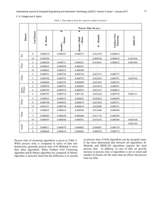
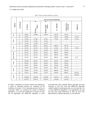
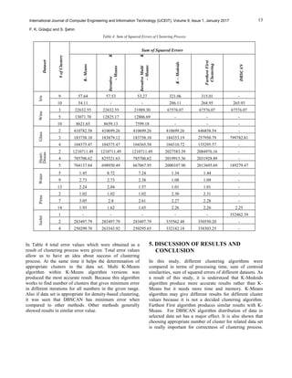
4. EXPERIMENTAL RESULTS
To evaluate the efficiency of the different clustering
algorithms, some tests are realized. Experimental tests are
realized on computer with Intel(R) Core(TM) i5-2410M
CPU @ 2.30 GHz, 4 GB RAM, 350 GB hard disk and
Windows 7 Ultimate operating system. While performing
the tests, six different algorithms were used. Analysis of
algorithms was made on seven different data sets as
mentioned section 2. Test process of algorithms was
carried out with Eclipse compiler and Java-ML (Java
Machine Learning Library) was used for implementation
of algorithms [21]. Table 2 shows results that contain
process time of algorithms, Table 3 shows the similarity of
centers and Table 4 shows results that contains total error
rate of algorithms.

6. 11International Journal of Computer Engineering and Information Technology (IJCEIT), Volume 9, Issue 1, January 2017
F. K. Gülağız and S. Şahin
Table 2: Time taken to form the respective number of clusters
Dataset
#ofClusters
Process Time (in sec.)
K-Means
IterativeK
-Means
IterativeMultiK
–Means
K–Medoids
FarthestFirst
Clustering
DBSCAN
Iris
9 0.000679 0.000553 0.000572 0.014359 0.000610 -
10 0.000784 - - 0.009520 0.000655 0.001058
Wine
3 0.000629 0.000711 0.000561 0.014691 0.000632 0.001049
5 0.000633 0.000594 0.000561 - - -
10 0.000622 0.000612 0.000588 - - -
Glass
2 0,000921 0,000726 0,000724 0,022212 0,000773 -
3 0,000766 0,000725 0,000795 0,022465 0,000761 0,001956
4 0,000668 0,000725 0,000890 0,023465 0,000743 -
Heart-
Diseas
2 0,000970 0,000781 0,000895 0,019614 0,000931 -
4 0,000795 0,000723 0,000933 0,021412 0,000813 -
5 0,000797 0,000714 0,001141 0,022244 0,000758 0,002131
Water
5 0,000833 0,000674 0,000681 0,020624 0,000659 -
9 0,000790 0,000692 0,000679 0,021894 0,000751 -
13 0,001011 0,000749 0,000619 0,022689 0,000731 -
Pima
2 0.000655 0.000614 0.000584 0.013468 0.000580 -
7 0.000603 0.000630 0.000600 0.011716 0.000594 -
14 0.000597 0.000568 0.000581 0.010192 0.000596 0.001038
Isolet
1 - - - - - 0.001102
2 0.000611 0.000678 0.000603 0.000481 0.000710 -
4 0.000646 0.000674 0.000642 0.000478 0.000772 -
Process time of clustering algorithms is given in Table 2.
When process time is compared in terms of data sets
dimensions, generally process time of K-Medoids is more
than other algorithms. When Farthest First Clustering
algorithm and K-Means algorithm are compared, K-Means
algorithm is narrowly faster but this difference is as second,
so process time of both algorithms can be accepted same.
It has been determined that between all algorithms, K-
Medoids and DBSCAN algorithms requires the most
process time. In addition, in case of data set growth,
increase in process time of algorithms is not so much and
number of clusters for the same data set effects the process
time too little.

7. 12International Journal of Computer Engineering and Information Technology (IJCEIT), Volume 9, Issue 1, January 2017
F. K. Gülağız and S. Şahin
Table 3: Sum of centroid similarities of clustersDataset
#ofClusters Sum of Centroid Similarities
K-Means
IterativeK
-Means
IterativeMultiK
–Means
K–Medoids
FarthestFirst
Clustering
DBSCAN
Iris
9 149.85 149.86 149.85 148.70 148.71 -
10 149.85 - - 148.82 148.88 131.89
Wine
3 177.80 177.80 177.81 177.83 177.83 177.83
5 177.82 177.82 177.82 - - -
10 177.86 177.86 177.87 - - -
Glass
2 209.48 209.41 209.41 209.41 205.74 -
3 211.84 211.74 211.84 211.69 211.95 171.86
4 212.83 212.83 212.69 212.72 212.61 -
Heart-Diseas
2 301.42 301.42 301.42 300.81 300.70 -
4 301.62 301.56 301.62 300.84 300.82 -
5 301.78 301.84 301.85 300.87 300.86 55.75
Water
5 526.80 526.81 526.79 526.03 526.04 -
9 526.82 526.82 526.82 526.05 526.07 -
13 526.83 526.85 526.82 526.05 526.09 -
Pima
2 726.95 726.95 726.95 688.77 687.84 -
7 750.30 751.39 750.29 690.49 689.78 -
14 752.45 758.48 757.92 691.09 690.91 687.54
Isolet
1 - - - - - 1136.89
2 1234.00 1234.00 1234.00 1165.24 1144.72 -
4 1274.67 1259.77 1259.74 1169.90 1161.63 -
In Table 3, similarities of clusters which were obtained as
a result of clustering process are evaluated. If the
similarity of centers is low clustering process will be so
successful. When we evaluated the results of different
algorithms, it is seen that similarities of centers are near
for all algorithms but DBSCAN algorithm is more
successful than other methods. When used data sets were
reviewed, it was also seen that DBSCAN algorithm
couldn’t perform clustering process in every data sets. As
a result, DBSCAN algorithm is not appropriate for data
sets that have high differences in data. In such case
determination of epsilon parameter is very difficult.

8. 13International Journal of Computer Engineering and Information Technology (IJCEIT), Volume 9, Issue 1, January 2017
F. K. Gülağız and S. Şahin
Table 4: Sum of Squared Errors of Clustering Process
Dataset
#ofClusters
Sum of Squared Errors
K-Means
IterativeK
-Means
IterativeMultiK
–Means
K–Medoids
FarthestFirst
Clustering
DBSCAN
Iris
9 57.64 57.53 53.27 321.06 315.01 -
10 54.11 - - 286.11 268.95 265.93
Wine
3 22632.55 22632.55 21989.30 67576.07 67576.07 67576.07
5 13071.70 12825.17 12806.69 - - -
10 8621.65 8659.13 7599.18 - - -
Glass
2 410782.58 410699.26 410699.26 410699.26 646858.54 -
3 183758.10 183879.12 183758.10 184353.19 257950.79 799782.81
4 104375.47 104375.47 104365.58 104310.72 135295.57 -
Heart-
Diseas
2 1210711.49 1210711.49 1210711.49 2027583.39 2084976.16 -
4 785706.62 825521.63 785706.62 2019915.36 2031928.89 -
5 704137.84 698950.49 667067.95 2000107.90 2013695.69 189279.47
Water
5 1.45 8.72 7.24 1.34 1.44 -
9 2.73 2.73 2.38 1.08 1.09 -
13 2.24 2.04 1.57 1.01 1.01 -
Pima
2 1.02 1.02 1.02 2.30 2.31 -
7 3.05 2.8 2.61 2.27 2.28 -
14 1.93 1.62 1.65 2.26 2.26 2.25
Isolet
1 - - - - - 352462.39
2 283497.79 283497.79 283497.79 335562.48 350550.20 -
4 250299.70 263343.92 250295.65 332182.18 338303.25 -
In Table 4 total error values which were obtained as a
result of clustering process were given. Total error values
allow us to have an idea about success of clustering
process. At the same time it helps the determination of
appropriate clusters in the data set. Multi K-Means
algorithm within K-Means algorithm versions was
produced the most accurate result. Because this algorithm
works to find number of clusters that gives minimum error
in different iterations for all numbers in the given range.
Also if data set is appropriate for density-based clustering,
it was seen that DBSCAN has minimum error when
compared to other methods. Other methods generally
showed results in similar error value.
5. DISCUSSION OF RESULTS AND
CONCLUSION
In this study, different clustering algorithms were
compared in terms of processing time, sum of centroid
similarities, sum of squared errors of different datasets. As
a result of this study, it is understood that K-Medoids
algorithm produce more accurate results rather than K-
Means but it needs more time and memory. K-Means
algorithm may give different results for different cluster
values because it is not a decided clustering algorithm.
Farthest First algorithm produces similar results with K-
Means. For DBSCAN algorithm distribution of data in
selected data set has a major effect. It is also shown that
choosing appropriate number of cluster for related data set
is really important for correctness of clustering process.

9. 14International Journal of Computer Engineering and Information Technology (IJCEIT), Volume 9, Issue 1, January 2017
F. K. Gülağız and S. Şahin
Considering all methods, DBSCSN algorithm gives the
most accurate results and K-Means is the fastest algorithm.
REFERENCES
[1] Alpaydın, E., Zeki Veri Madenciliği: Ham Veriden Altın
Bilgiye Ulaşma Yöntemler, Bilişim 2000, Veri
madenciliği Eğitim Semineri, 2000.
[2] Özkan, Y., Veri Madenciliği Yöntemleri, Papatya
Yayıncılık, İstanbul, Turkey, 2008.
[3] Ibaraki, M., Data Mining Techniques for Associations,
Clustering and Classification Methodologies, PAKDD'99,
In: Proceedings of Third Pacific-Asia Conference, 1999,
pp 13-23.
[4] Savaş, S., Topaloğlu, N., Yılmaz, M., Veri Madenciliği ve
Türkiye’ deki Uygulama Örnekleri, İstanbul Ticaret
Üniversitesi Fen Bilimleri Dergisi, 2012, 11 (21), pp 1-23.
[5] Deza, M. M., Deza, E., Encyclopedia of Distance,
Springer, 2009.
[6] Çoşlu, E., Veri Madenciliği, In: Proceedings of Akademik
Bilişim 2013 Conference, 2013, pp 573-585
[7] Taşkın, Ç., Emel, G. G., Veri Madenciliğinde Kümeleme
Yaklaşimlari Ve Kohonen Ağlari İle Perakendecilik
Sektöründe Bir Uygulama, Süleyman Demirel
Üniversitesi İktisadi ve İdari Bilimler Fakültesi Dergisi,
2010, 15(3), pp 395-409.
[8] Eden, M. A., Tommy, W. S., A New Shifting Grid
Clustering Algorithm, Pattern Recognition, 2004, 37(3),
pp 503-514.
[9] Kuo, R. J., Ho, L. M., Hu, C. M., Cluster Analysis in
Industrial Market Segmentation Through Artificial Neural
Network, Computers & Industrial Engineering, 2002,
42(2-4), pp 391-399.
[10] Likas, A., Vlassisb, N., Verbeekb, J. J., The Global K-
Means Clustering Algorithm, Pattern Recognition, 2003,
36(2), pp 451-461.
[11] Hsu, C. H., Data Mining to Improve Industrial Standards
and Enhance Production and Marketing: An Empirical
Study in Apparel Industry, Expert Systems with
Applications, 2003, 36(3), pp 4185–4191.
[12] Kaya, H., Köymen, K., Veri Madenciliği Kavrami Ve
Uygulama Alanlari, Doğu Anadolu Bölgesi Araştırmları,
2008.
[13] R. Capaldo and F. Collova, Clustering: A survey,
http://www.slideshare.net/rcapaldo/cluster-analysis-
presentation, (2008).
[14] Kaufman, L., Rousseeuw, P. J., Clustering by Means of
Medoids, Statistical Data Analysis Based on The L1–
Norm and Related Methods, Springer, 1987.
[15] Kaufman, L., Rousseeuw, P. J., Finding Groups in Data:
An Introduction to Cluster Analysis, Wiley, 1990.
[16] Işık, M.,Çanurcu, A., K-Means, K-Medoids Ve Bulanik
C-Means Algoritmalarinin Uygulamali Olarak
Performanslarinin Tespiti, İstanbul Ticaret Üniversitesi
Fen Bilimleri Dergisi, 2007, 6(11), pp 31-45
[17] Sharmila, Kumar, M., An Optimized Farthest First
Clustering Algorithm, In: Proceedings of Nirma
University International Conference on Engineering,
2013, pp 1-5.
[18] Bilgin, T. T., Çamurcu, Y., DBSCAN, OPTICS ve K-
Means Kümeleme Algoritmalarının Uygulamalı
Karşılaştırılması, Politeknik Dergisi, 2005, 8(2), pp 139-
145.
[19] Lichman, M. (2013). UCI Machine Learning Repository
[http://archive.ics.uci.edu/ml]. Irvine, CA: University of
California, School of Information and Computer Science.
[20] Dziak, J. J., Coffman, D. L., Lanza, S. T., Li, R.,
Sensitivity and Specificity of Information Criteria,
Technical Report Series #12-119, The Pennsylvania State
University, College of Health and Human Development,
Metodology Center.
[21] Abeel, T., Peer, Y. V., Saeys, Y., Java-ML: A Machine
Learning Library, Journal of Machine Learning Research,
2009, 10, pp 931-934.
AUTHOR PROFILES:
Fidan Kaya Gülağız has received her BEng. in Computer
Engineering from Kocaeli University in 2010 and ME. in
Computer Engineering from Kocaeli University in 2012. She is
currently working towards Ph.D. degree in Computer
Engineering from Kocaeli University, Turkey. Also, she is
currently a Research Assistant of Computer Engineering
Department at Kocaeli University in Turkey. Her main
research interests include data synchronization, distributed file
systems and data filtering methods.
Suhap Şahin has received his BEng. in Electrical, Electronics
and Communications Engineering from Kocaeli University in
2000. He is an associate professor at the Kocaeli University
Computer Engineering Department in Turkey. He has a Ph.D.
at the Kocaeli University Electrical, Electronics and
Communications Engineering. His main research interests
include beamforming, FPGA, OFDM and wireless
communication.