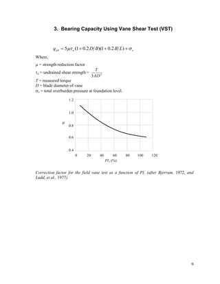
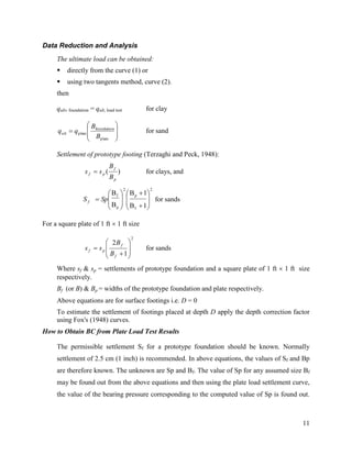
SlideShare a Scribd company logo
1
BEARING CAPACITY BASED ON IN-SITU AND LABORATORY TESTS
IN-SITU TESTS
BC can be estimated by in-situ and laboratory tests, the most common in-situ tests for BC
evaluation are
 Standard Penetration Test (SPT), very cheap, most common and popular
 Cone Penetration Test (CPT), very sophisticated, costly, not very common as compared
with SPT
 Vane shear Test
SPT
SPT-N Value:
Number of blows required for
12 inch penetration of split
spoon sampler under the impact
of a standard wt. of 140 lbs
dropped from a height of 30
inch
2
 It consists of penetrating a sampler known as split spoon sampler by dropping a standard
weight of 140 lbs by 30 inch height. The sampler is penetrating by 18 inches total and for
each 6 inches; the number of blows required for each of the penetration are counted
separately. The number of blows for first 6 inches is ignored and the total numbers of
blows for next two 6 inch penetration (total 12 inch) are taken and known as SPT-N
value. (e.g. if the respective blow count for three successive 6 inch penetration are 8, 9,
10 then SPT-N value is 19.)
 As a part of test, the representative but disturbed soil sample is procured at the test depth
for laboratory testing.
 SPT is generally performed at every 1 m interval up to 15~20 m and then interval may
be increased to 1.5-2 m.
 If SPT is performed below GWT, the SPT-N values is overestimated and a correction to
measured N is (dilatancy correction) applied if SPT-N value exceeds 15
Ncorr. = 15 + 0.5(Nmeasured -15)
 The SPT is more reliable for granular soils as compared with fine grained soils.
 In case of gravels, a 60o
cone is used in stead of split spoon samples
 If SPT is performed below GWT, sand boiling causes disturbance leading to erroneous
SPT-N values. The borehole casing should be filled with water all the time to avoid sand
boiling in case of light percussion technique.
 The SPT-N value has the following correlation with different parameters.
3
GRANULAR SOILS
Description Very Loose Loose Medium Dense Very Dense
Relative density, Dr 0 – 0.15 0.15 – 0.35 0.35 – 0.65 0.65 – 0.85 0.85 – 1.00
Standard Penetration Test
value, N
0 – 4 5 – 10 11 – 30 31 – 50 51 – UP
Approximate angle of internal
friction, degree)
25 – 28 28 – 30 30 – 35 35 – 40 38 – 43
Approximate range of moist
unit weight,  (pcf)
70 – 100 90 – 115 110 – 130 110 – 140 130 – 150
Submerged unit weight, sub 60 55 – 65 60 – 70 65 – 85 75
COHESIVE SOILS
Description Very
Soft
Soft Firm Stiff Very Stiff Hard
Unconfined compressive
strength, qu (tsf)
0 – 0.25 0.25 – 0.5 0.5 – 1.0 1.0 – 2.0 2.0 – 4.0 4.0 – UP
Standard Penetration Test
value, N
0 – 2 3 – 4 5 – 8 9 – 16 17 – 32 33 – UP
Approx. range of saturated unit
weight, sat (pcf)
100 – 120 100 – 130 120 – 140 130+
4
1. Bearing Capacity from SPT
a. Terzaghi & Peck (1948) Method
Terzaghi & Peck (1948) were first to propose a correlation between SPT-N value and allowable
pressure for a settlement of 25 mm (1 inch). The estimation of qa is considered to be very
conservative and is generally not used by current practitioners. The equation is as inder:
  w
d
a R
K
B
B
N
q 





 


2
2
1
3
720 N > 3
where qa = net allowable bearing pressure in psf for 1 inch settlement and B in ft.
or   w
d
a R
K
B
B
N
q 





 


2
2
305
.
0
3
5
.
34 , qa in kPa, B in m
33
.
1
)
33
.
0
1
( 


B
D
Kd , (for R’w see Fig. 1)
This equation can be modified for calculation of settlement for any given pressure
  w
d K
qC
B
B
N
s
2
305
.
0
3
9
.
2








 s in mm, B in m and q in kPa
Cd = 1 for D/B = 0 Cd = 0.75 for D/B = 1
Kw = 1 for Dw > B Kw = 2.0 for Dw = 0
b. Meyerhof (1956) method:
(SI units) qa = 12 N Kd for B1.2 m
(Fps units) qa = d
K
N
4
for B < 4 ft
(SI units) qa= d
K
B
B
N
2
3
.
0
8 




 
for B > 1.2 m
(Fps units) qa = d
K
B
B
N
2
1
6





 
for B > 4 ft
5
Where,
qa = allowable bearing pressure for a maximum settlement of 25 mm or 1-inch, kPa or ksf.
N = SPT resistance in blows/300 mm = statistical average value for the footing influence zone
of about 0.5B above footing base to at least 2B below.
B = footing width in meters or feet.
Kd = depth factor = 33
.
1
)
33
.
0
1
( 

B
D
For any settlement, actual
a
actual q
q
s
s 
For s = 25 mm, the above equations (in SI units) can be modified to determine settlement under
the known contact pressure or vice versa as below:
actual
actual
2
q
C
N
s d
 for B  1.2 m
actual
2
actual
3
.
0
12
.
3
q
C
B
B
N
s d







 for B > 1.2 m
Where
B
D
K
C
d
d
33
.
0
1
1
1


  0.75 and  1.0
c. Meyerhof method modified by Bowles (1977):
(SI units) qa = 20 N Kd for B1.2 m
(Fps units) qa = d
K
N
5
.
2
for B < 4 ft
(SI units) qa.= d
K
B
B
N
2
3
.
0
5
.
12 




 
for B > 1.2 m
(Fps units) qa = d
K
B
B
N
2
1
4





 
for B > 4 ft
Where,
qa = allowable bearing pressure for a maximum settlement of 25 mm or 1-inch, kPa or ksf.
N = SPT resistance in blows/300 mm = statistical average value for the footing influence zone
of about 0.5B above footing base to at least 2B below.
6
B = footing width in meters or feet.
Kd = depth factor = 33
.
1
)
33
.
0
1
( 

B
D
For any settlement, actual
a
actual q
q
s
s 
For s = 25 mm, the above equations (in SI units) can be modified to determine settlement under
the known contact pressure or vice versa as below:
actual
actual
25
.
1
q
C
N
s d
 for B  1.2 m
actual
2
actual
3
.
0
2
q
C
B
B
N
s d







 for B > 1.2 m
Where
B
D
K
C
d
d
33
.
0
1
1
1


  0.75 and  1.0
d. Teng (1962) Relations based on shear failure criterion
For strip footing:
)
100
(
5
3 2
2
w
w
ult DR
N
R
BN
q 


 (Fps units)
The above equation may be modified for qs (FS=3) in SI units
)
100
(
262
.
0
157
.
0 2
2
w
w
s DR
N
R
BN
q 


 (SI units)
For square footing:
)
100
(
6
2 2
2
w
w
ult DR
N
R
BN
q 


 (Fps units)
The above equation may be modified for qs (FS=3) in SI units
)
100
(
314
.
0
105
.
0 2
2
w
w
s DR
N
R
BN
q 


 (SI units)
Where,
qs = net safe bearing capacity w.r.t. shear failure alone for FOS of 3 in psf or kPa
B = footing width in ft or meters
N = SPT resistance in blows/300 mm
D = footing depth in ft or meters; if D > B use D = B for computation
7
Rw & R'w = water table reduction factor
B
D
db
a
d
B
Water
Table
Water Table
Footing
(a)
0 0.2 0.4 0.6 0.8 1.0
0.5
0.6
0.7
0.8
0.9
1.0
Reduction factor,
R w
0 0.2 0.4 0.6 0.8 1.0
0.5
0.6
0.7
0.8
0.9
1.0
Reduction factor,
R' w
(b) (c)
d /D d /B
a b
f
f
R = 1 - 0.5
w
d a
Df
R' w = 0.5 + 0.5
d
B
b
Fig. 1: Correction factors for position of water level: (a) depth of water level with respect
to dimension of footing; (b) water level above base of footing; (c) water level below base of
footing.
e. Parry (1977) Relation based on shear failure criterion
For cohesionless soils only
qult = 30 N (kPa) (D  B)
N = average SPT value at a depth about 0.75B below the proposed base of the footing.
8
2. Bearing Capacity using CPT
(i) Meyerhof (1956)
For a maximum settlement of 25 mm; for foundations (strip or square) on dry sands:
qa= 3.6 qc kN/m2
 qc/30 kg/cm2
for B  1.2 m
qa= 2.1 qc (1 + 1/B)2
kN/m2
 qc/50 (1 + 1/B)2
kg/cm2
for B > 1.2 m
For any value of B, an approximate formula is:
qa= 2.7 qc kN/m2
= qc/40 kg/cm2
Where,
qa = allowable pressure for 25 mm
B = footing width in meters.
qc = CPT cone resistance in kPa.
Notes:
 above equations are based on the approximate rule that N =qc/4 (in kg/cm2
).
 qa is halved if the sand within the stresses zone is submerged.
 For rafts and pier foundations, double the qa values determined above.
(ii) Schmertmann (1978)
The bearing capacity factors for use in Terzaghi's bearing capacity equation can be
estimated as:
0.8 Nq  0.8 N  qc D/B  1.5.
Where qc is average cone resistance over depth interval from B/2 above to 1.1B below
footing base.
 For Cohesionless Soils
Strip: 2
5
.
1
ult kg/cm
in
)
300
(
0052
.
0
28 c
q
q 

 or tons/ft2
Square: 2
5
.
1
ult kg/cm
in
)
300
(
009
.
0
48 c
q
q 

 or tons/ft2
 For Cohesive Soils
Strip: 2
kg/cm
in
28
.
0
2 c
ult q
q 
 or tons/ft2
Square 2
kg/cm
in
34
.
0
5 c
ult q
q 
 or tons/ft2
9
3. Bearing Capacity Using Vane Shear Test (VST)
v
u
ult L
B
B
D
q 
 


 )
2
.
0
1
)(
2
.
0
1
(
5
Where,
 = strength reduction factor
u = undrained shear strength = 3
6
.
3 D
T
T = measured torque
D = blade diameter of vane
v = total overburden pressure at foundation level.
1.2
1.0
0.8
0.6
0.4
0 20 40 60 80 100 120

PI, (%)
Correction factor for the field vane test as a function of PI, (after Bjerrum, 1972, and
Ladd, et al., 1977).
10
4. BEARING CAPACITY FROM PLATE LOAD TEST
Dead Weight
Pit
Rigid Steel Plate
of Square Shape
Hydraulic Jack with
Loading Cell
Loading
Frame
Three Settlement
Dial Gauges Spaced
at 120 apart approx.
o
Schematic sketch showing load-test arrangement
For details of equipment and testing procedure, refer to ASTM D 1195
 The load is applied in increments of 25% of the proposed design load.
 Increments are added till the final load is 150 to 200% of the proposed design load or
to the failure of the soil underneath the plate.
 Each increment of load is maintained until the settlement is ceased, however the final
applied load is maintained for not less than 24 hours.
 Settlement dial readings are recorded for each load increment after 5, 10, 15, 30, 60
minutes and every 1 hour interval thereafter to the first 6 hours and at least once every
12 hours thereafter.
1
2
P Pu
u
= Ultimate Load
Load
Settlement
Typical load-settlement plots of a load test
11
Data Reduction and Analysis
The ultimate load can be obtained:
 directly from the curve (1) or
 using two tangents method, curve (2).
then
qult, foundation = qult, load test for clay









plate
foundation
plate
ult
B
B
q
q for sand
Settlement of prototype footing (Terzaghi and Peck, 1948):
)
(
p
f
p
f
B
B
s
s  for clays, and
2
f
p
2
p
f
1
B
1
B
B
B


















 Sp
S f for sands
For a square plate of 1 ft  1 ft size
2
1
2










f
f
p
f
B
B
s
s for sands
Where sf & sp = settlements of prototype foundation and a square plate of 1 ft  1 ft size
respectively.
Bf (or B) & Bp = widths of the prototype foundation and plate respectively.
Above equations are for surface footings i.e. D = 0
To estimate the settlement of footings placed at depth D apply the depth correction factor
using Fox's (1948) curves.
How to Obtain BC from Plate Load Test Results
The permissible settlement Sf for a prototype foundation should be known. Normally
settlement of 2.5 cm (1 inch) is recommended. In above equations, the values of Sf and Bp
are therefore known. The unknown are Sp and Bf. The value of Sp for any assumed size Bf
may be found out from the above equations and then using the plate load settlement curve,
the value of the bearing pressure corresponding to the computed value of Sp is found out.
12
The bearing pressure is the allowable bearing pressure for a given permissible settlement
Sf.
Limitation of the Plate Load Test
1. Since plate load test is of short duration, it will not give consolidation settlement. If the
underlying soil is sandy in nature immediate settlement may be taken as the total
settlement. If the soil is clayey type, the immediate settlement is only a fraction of the total
settlement. Load tests, therefore, do not have much significance in clayey soils to
determine allowable pressure on the basis of settlement criterion.
2. Plate load tests should be used with caution and the present practice is not to rely too
much on this test. If the soil is not homogeneous to a great depth, plate load tests give very
misleading results.
Assume two layers of soil. The top layer is stiff clay where as the bottom layer is soft clay.
The load test conducted near the surface of the ground measures the characteristics of stiff
clay but does not indicate the nature of the soft clay soil which is below. The actual
foundation of a building, however, has a bulb of pressure which extends to a great depth
into the poor soil which is highly compressible. Whereas the soil tested by the plate load
test is very good leading to unsafe design. Plate load test is, therefore, not at all
Soil-1, stiff clay
Soil-2, soft clay
13
recommended on soils, which are not homogeneous at least to a depth equal to 1.5 to 2
times the width of the prototype foundation.
3. Plate load tests should not be relied on to determine the ultimate B.C of sandy soils as
the scale (size) effect gives very misleading results. However, when the tests are carried on
clay soils, the ultimate B.C as determined by the test may be taken as equal to that of the
foundation since the bearing of clay is essentially independent of the footing size
5. BY LABORATORY UNCONFINED COMPRESSION TEST
The B.C of a cohesive soil can also be evaluated from the unconfined compressive test
on cohesive soils. The failure axial stress in case of unconfined compression test is
termed as unconfined compressive stress which is equal to:
qu = 2C
and C = qu/2 and  =0 (for undrained condition)
By Terzaghi’s equation, the BC of cohesive soils for  =0 case is
qun = CNc Nc = 5.7 or approximately 6
qun = 6C
for FS=3
qns = 2C = qu
Therefore, the net safe bearing capacity (qns) of cohesive soil can be taken approximately
equal to unconfined compression strength of cohesive soil.
6. BC BY BUILDING CODES:
In many countries/cities, the local building code stipulates values of allowable soil pressure to
use when designing foundations. These values are usually based on years of experience,
although in some cases they are simply used from the building construction handbooks.
14
These arbitrary values of soil pressure are termed as Presumptive Bearing Pressures. The
presumptive pressures are generally based on a visual soil classification. Following table
summaries the Presumptive Bearing Pressures from the International Building Code.
Table: Presumptive Bearing Pressures from the International Building Code (IBC, 1997)
Soil or Rock Classification Allowable Bearing Pressure, qa
(kPa) (lbs/ft2
)
Crystalline Bedrock 600 12,000
Sedimentary or Foliated Rocks 300 6,000
Sandy gravel, or gravel (GW, GP) 250 5,000
Sand, silty Sand, clayey sand, silty gravel,
clayey gravel, (SW, SP, SM, SC, GM and
GC)
150 3,000
Clay, sandy clay, silty clay, or clayey silt,
(CL, ML, MH, CH)
100 2,000
Mud, organic silt, organic clay, peat or
unprepared fill
0 0

More Related Content

Similar to 6._Bearing_Capacity_from_other_methods.pdf

1.4 latifs 17 dramix sog
1.4 latifs 17 dramix sog 1.4 latifs 17 dramix sog
1.4 latifs 17 dramix sog
Latifs Chile
 
Precast driven pile 450 x450
Precast driven pile 450 x450Precast driven pile 450 x450
Precast driven pile 450 x450
Priodeep Chowdhury
 
기초공학 - 11-2 Pile Foundations.pdf
기초공학 - 11-2 Pile Foundations.pdf기초공학 - 11-2 Pile Foundations.pdf
기초공학 - 11-2 Pile Foundations.pdf
ShallomNkhoma
 
Coiled tubing calculations.pdf
Coiled tubing calculations.pdfCoiled tubing calculations.pdf
Coiled tubing calculations.pdf
JesusCubillas1
 
Pe Test Geotechnical Rerview
Pe Test Geotechnical RerviewPe Test Geotechnical Rerview
Pe Test Geotechnical Rerview
imedlachheb
 
Gate 2017 me 1 solutions with explanations
Gate 2017 me 1 solutions with explanationsGate 2017 me 1 solutions with explanations
Gate 2017 me 1 solutions with explanations
kulkarni Academy
 
Gate 2017 me 1 solutions with explanations
Gate 2017 me 1 solutions with explanationsGate 2017 me 1 solutions with explanations
Gate 2017 me 1 solutions with explanations
kulkarni Academy
 
Deber corte
Deber corteDeber corte
Deber corte
AldoChandiAngulo
 
Ans1
Ans1Ans1
Solution to-2nd-semester-soil-mechanics-2015-2016
Solution to-2nd-semester-soil-mechanics-2015-2016Solution to-2nd-semester-soil-mechanics-2015-2016
Solution to-2nd-semester-soil-mechanics-2015-2016
chener Qadr
 
Rc19 footing1
Rc19 footing1Rc19 footing1
Rc19 footing1
bayan mostafa
 
Foundationeng deep-foundations_ps
Foundationeng deep-foundations_psFoundationeng deep-foundations_ps
Foundationeng deep-foundations_ps
İsimsiz Kahraman
 
Chapter 2 free vibration of single degree of freedom
Chapter 2 free vibration of single degree of freedomChapter 2 free vibration of single degree of freedom
Chapter 2 free vibration of single degree of freedom
Rafi sulaiman
 
Standard_Penetration_Test__SPT_.pptx
Standard_Penetration_Test__SPT_.pptxStandard_Penetration_Test__SPT_.pptx
Standard_Penetration_Test__SPT_.pptx
TabRasa1
 
Problems on bearing capacity of soil
Problems on bearing capacity of soilProblems on bearing capacity of soil
Problems on bearing capacity of soil
Latif Hyder Wadho
 
Lateral Earth pressure
Lateral Earth pressureLateral Earth pressure
Lateral Earth pressure
Latif Hyder Wadho
 
Margen izquierdo ok
Margen izquierdo okMargen izquierdo ok
Margen izquierdo ok
FritzDelRoAltamirano
 
04 ec2 ws_walraven_ulssls
04 ec2 ws_walraven_ulssls04 ec2 ws_walraven_ulssls
04 ec2 ws_walraven_ulssls
luantvconst
 
Fellenius prediction presentation
Fellenius  prediction presentationFellenius  prediction presentation
Fellenius prediction presentation
cfpbolivia
 
Unisoft software bengt h. fellenius, pierre goudrault
Unisoft software   bengt h. fellenius, pierre goudraultUnisoft software   bengt h. fellenius, pierre goudrault
Unisoft software bengt h. fellenius, pierre goudrault
cfpbolivia
 

Similar to 6._Bearing_Capacity_from_other_methods.pdf (20)

1.4 latifs 17 dramix sog
1.4 latifs 17 dramix sog 1.4 latifs 17 dramix sog
1.4 latifs 17 dramix sog
 
Precast driven pile 450 x450
Precast driven pile 450 x450Precast driven pile 450 x450
Precast driven pile 450 x450
 
기초공학 - 11-2 Pile Foundations.pdf
기초공학 - 11-2 Pile Foundations.pdf기초공학 - 11-2 Pile Foundations.pdf
기초공학 - 11-2 Pile Foundations.pdf
 
Coiled tubing calculations.pdf
Coiled tubing calculations.pdfCoiled tubing calculations.pdf
Coiled tubing calculations.pdf
 
Pe Test Geotechnical Rerview
Pe Test Geotechnical RerviewPe Test Geotechnical Rerview
Pe Test Geotechnical Rerview
 
Gate 2017 me 1 solutions with explanations
Gate 2017 me 1 solutions with explanationsGate 2017 me 1 solutions with explanations
Gate 2017 me 1 solutions with explanations
 
Gate 2017 me 1 solutions with explanations
Gate 2017 me 1 solutions with explanationsGate 2017 me 1 solutions with explanations
Gate 2017 me 1 solutions with explanations
 
Deber corte
Deber corteDeber corte
Deber corte
 
Ans1
Ans1Ans1
Ans1
 
Solution to-2nd-semester-soil-mechanics-2015-2016
Solution to-2nd-semester-soil-mechanics-2015-2016Solution to-2nd-semester-soil-mechanics-2015-2016
Solution to-2nd-semester-soil-mechanics-2015-2016
 
Rc19 footing1
Rc19 footing1Rc19 footing1
Rc19 footing1
 
Foundationeng deep-foundations_ps
Foundationeng deep-foundations_psFoundationeng deep-foundations_ps
Foundationeng deep-foundations_ps
 
Chapter 2 free vibration of single degree of freedom
Chapter 2 free vibration of single degree of freedomChapter 2 free vibration of single degree of freedom
Chapter 2 free vibration of single degree of freedom
 
Standard_Penetration_Test__SPT_.pptx
Standard_Penetration_Test__SPT_.pptxStandard_Penetration_Test__SPT_.pptx
Standard_Penetration_Test__SPT_.pptx
 
Problems on bearing capacity of soil
Problems on bearing capacity of soilProblems on bearing capacity of soil
Problems on bearing capacity of soil
 
Lateral Earth pressure
Lateral Earth pressureLateral Earth pressure
Lateral Earth pressure
 
Margen izquierdo ok
Margen izquierdo okMargen izquierdo ok
Margen izquierdo ok
 
04 ec2 ws_walraven_ulssls
04 ec2 ws_walraven_ulssls04 ec2 ws_walraven_ulssls
04 ec2 ws_walraven_ulssls
 
Fellenius prediction presentation
Fellenius  prediction presentationFellenius  prediction presentation
Fellenius prediction presentation
 
Unisoft software bengt h. fellenius, pierre goudrault
Unisoft software   bengt h. fellenius, pierre goudraultUnisoft software   bengt h. fellenius, pierre goudrault
Unisoft software bengt h. fellenius, pierre goudrault
 

Recently uploaded

学校原版美国波士顿大学毕业证学历学位证书原版一模一样
学校原版美国波士顿大学毕业证学历学位证书原版一模一样学校原版美国波士顿大学毕业证学历学位证书原版一模一样
学校原版美国波士顿大学毕业证学历学位证书原版一模一样
171ticu
 
一比一原版(CalArts毕业证)加利福尼亚艺术学院毕业证如何办理
一比一原版(CalArts毕业证)加利福尼亚艺术学院毕业证如何办理一比一原版(CalArts毕业证)加利福尼亚艺术学院毕业证如何办理
一比一原版(CalArts毕业证)加利福尼亚艺术学院毕业证如何办理
ecqow
 
Engineering Standards Wiring methods.pdf
Engineering Standards Wiring methods.pdfEngineering Standards Wiring methods.pdf
Engineering Standards Wiring methods.pdf
edwin408357
 
Curve Fitting in Numerical Methods Regression
Curve Fitting in Numerical Methods RegressionCurve Fitting in Numerical Methods Regression
Curve Fitting in Numerical Methods Regression
Nada Hikmah
 
一比一原版(爱大毕业证书)爱荷华大学毕业证如何办理
一比一原版(爱大毕业证书)爱荷华大学毕业证如何办理一比一原版(爱大毕业证书)爱荷华大学毕业证如何办理
一比一原版(爱大毕业证书)爱荷华大学毕业证如何办理
nedcocy
 
IEEE Aerospace and Electronic Systems Society as a Graduate Student Member
IEEE Aerospace and Electronic Systems Society as a Graduate Student MemberIEEE Aerospace and Electronic Systems Society as a Graduate Student Member
IEEE Aerospace and Electronic Systems Society as a Graduate Student Member
VICTOR MAESTRE RAMIREZ
 
Advanced control scheme of doubly fed induction generator for wind turbine us...
Advanced control scheme of doubly fed induction generator for wind turbine us...Advanced control scheme of doubly fed induction generator for wind turbine us...
Advanced control scheme of doubly fed induction generator for wind turbine us...
IJECEIAES
 
LLM Fine Tuning with QLoRA Cassandra Lunch 4, presented by Anant
LLM Fine Tuning with QLoRA Cassandra Lunch 4, presented by AnantLLM Fine Tuning with QLoRA Cassandra Lunch 4, presented by Anant
LLM Fine Tuning with QLoRA Cassandra Lunch 4, presented by Anant
Anant Corporation
 
22CYT12-Unit-V-E Waste and its Management.ppt
22CYT12-Unit-V-E Waste and its Management.ppt22CYT12-Unit-V-E Waste and its Management.ppt
22CYT12-Unit-V-E Waste and its Management.ppt
KrishnaveniKrishnara1
 
Redefining brain tumor segmentation: a cutting-edge convolutional neural netw...
Redefining brain tumor segmentation: a cutting-edge convolutional neural netw...Redefining brain tumor segmentation: a cutting-edge convolutional neural netw...
Redefining brain tumor segmentation: a cutting-edge convolutional neural netw...
IJECEIAES
 
Properties Railway Sleepers and Test.pptx
Properties Railway Sleepers and Test.pptxProperties Railway Sleepers and Test.pptx
Properties Railway Sleepers and Test.pptx
MDSABBIROJJAMANPAYEL
 
4. Mosca vol I -Fisica-Tipler-5ta-Edicion-Vol-1.pdf
4. Mosca vol I -Fisica-Tipler-5ta-Edicion-Vol-1.pdf4. Mosca vol I -Fisica-Tipler-5ta-Edicion-Vol-1.pdf
4. Mosca vol I -Fisica-Tipler-5ta-Edicion-Vol-1.pdf
Gino153088
 
Software Engineering and Project Management - Introduction, Modeling Concepts...
Software Engineering and Project Management - Introduction, Modeling Concepts...Software Engineering and Project Management - Introduction, Modeling Concepts...
Software Engineering and Project Management - Introduction, Modeling Concepts...
Prakhyath Rai
 
DEEP LEARNING FOR SMART GRID INTRUSION DETECTION: A HYBRID CNN-LSTM-BASED MODEL
DEEP LEARNING FOR SMART GRID INTRUSION DETECTION: A HYBRID CNN-LSTM-BASED MODELDEEP LEARNING FOR SMART GRID INTRUSION DETECTION: A HYBRID CNN-LSTM-BASED MODEL
DEEP LEARNING FOR SMART GRID INTRUSION DETECTION: A HYBRID CNN-LSTM-BASED MODEL
ijaia
 
Optimizing Gradle Builds - Gradle DPE Tour Berlin 2024
Optimizing Gradle Builds - Gradle DPE Tour Berlin 2024Optimizing Gradle Builds - Gradle DPE Tour Berlin 2024
Optimizing Gradle Builds - Gradle DPE Tour Berlin 2024
Sinan KOZAK
 
Rainfall intensity duration frequency curve statistical analysis and modeling...
Rainfall intensity duration frequency curve statistical analysis and modeling...Rainfall intensity duration frequency curve statistical analysis and modeling...
Rainfall intensity duration frequency curve statistical analysis and modeling...
bijceesjournal
 
Applications of artificial Intelligence in Mechanical Engineering.pdf
Applications of artificial Intelligence in Mechanical Engineering.pdfApplications of artificial Intelligence in Mechanical Engineering.pdf
Applications of artificial Intelligence in Mechanical Engineering.pdf
Atif Razi
 
Digital Twins Computer Networking Paper Presentation.pptx
Digital Twins Computer Networking Paper Presentation.pptxDigital Twins Computer Networking Paper Presentation.pptx
Digital Twins Computer Networking Paper Presentation.pptx
aryanpankaj78
 
ITSM Integration with MuleSoft.pptx
ITSM  Integration with MuleSoft.pptxITSM  Integration with MuleSoft.pptx
ITSM Integration with MuleSoft.pptx
VANDANAMOHANGOUDA
 
132/33KV substation case study Presentation
132/33KV substation case study Presentation132/33KV substation case study Presentation
132/33KV substation case study Presentation
kandramariana6
 

Recently uploaded (20)

学校原版美国波士顿大学毕业证学历学位证书原版一模一样
学校原版美国波士顿大学毕业证学历学位证书原版一模一样学校原版美国波士顿大学毕业证学历学位证书原版一模一样
学校原版美国波士顿大学毕业证学历学位证书原版一模一样
 
一比一原版(CalArts毕业证)加利福尼亚艺术学院毕业证如何办理
一比一原版(CalArts毕业证)加利福尼亚艺术学院毕业证如何办理一比一原版(CalArts毕业证)加利福尼亚艺术学院毕业证如何办理
一比一原版(CalArts毕业证)加利福尼亚艺术学院毕业证如何办理
 
Engineering Standards Wiring methods.pdf
Engineering Standards Wiring methods.pdfEngineering Standards Wiring methods.pdf
Engineering Standards Wiring methods.pdf
 
Curve Fitting in Numerical Methods Regression
Curve Fitting in Numerical Methods RegressionCurve Fitting in Numerical Methods Regression
Curve Fitting in Numerical Methods Regression
 
一比一原版(爱大毕业证书)爱荷华大学毕业证如何办理
一比一原版(爱大毕业证书)爱荷华大学毕业证如何办理一比一原版(爱大毕业证书)爱荷华大学毕业证如何办理
一比一原版(爱大毕业证书)爱荷华大学毕业证如何办理
 
IEEE Aerospace and Electronic Systems Society as a Graduate Student Member
IEEE Aerospace and Electronic Systems Society as a Graduate Student MemberIEEE Aerospace and Electronic Systems Society as a Graduate Student Member
IEEE Aerospace and Electronic Systems Society as a Graduate Student Member
 
Advanced control scheme of doubly fed induction generator for wind turbine us...
Advanced control scheme of doubly fed induction generator for wind turbine us...Advanced control scheme of doubly fed induction generator for wind turbine us...
Advanced control scheme of doubly fed induction generator for wind turbine us...
 
LLM Fine Tuning with QLoRA Cassandra Lunch 4, presented by Anant
LLM Fine Tuning with QLoRA Cassandra Lunch 4, presented by AnantLLM Fine Tuning with QLoRA Cassandra Lunch 4, presented by Anant
LLM Fine Tuning with QLoRA Cassandra Lunch 4, presented by Anant
 
22CYT12-Unit-V-E Waste and its Management.ppt
22CYT12-Unit-V-E Waste and its Management.ppt22CYT12-Unit-V-E Waste and its Management.ppt
22CYT12-Unit-V-E Waste and its Management.ppt
 
Redefining brain tumor segmentation: a cutting-edge convolutional neural netw...
Redefining brain tumor segmentation: a cutting-edge convolutional neural netw...Redefining brain tumor segmentation: a cutting-edge convolutional neural netw...
Redefining brain tumor segmentation: a cutting-edge convolutional neural netw...
 
Properties Railway Sleepers and Test.pptx
Properties Railway Sleepers and Test.pptxProperties Railway Sleepers and Test.pptx
Properties Railway Sleepers and Test.pptx
 
4. Mosca vol I -Fisica-Tipler-5ta-Edicion-Vol-1.pdf
4. Mosca vol I -Fisica-Tipler-5ta-Edicion-Vol-1.pdf4. Mosca vol I -Fisica-Tipler-5ta-Edicion-Vol-1.pdf
4. Mosca vol I -Fisica-Tipler-5ta-Edicion-Vol-1.pdf
 
Software Engineering and Project Management - Introduction, Modeling Concepts...
Software Engineering and Project Management - Introduction, Modeling Concepts...Software Engineering and Project Management - Introduction, Modeling Concepts...
Software Engineering and Project Management - Introduction, Modeling Concepts...
 
DEEP LEARNING FOR SMART GRID INTRUSION DETECTION: A HYBRID CNN-LSTM-BASED MODEL
DEEP LEARNING FOR SMART GRID INTRUSION DETECTION: A HYBRID CNN-LSTM-BASED MODELDEEP LEARNING FOR SMART GRID INTRUSION DETECTION: A HYBRID CNN-LSTM-BASED MODEL
DEEP LEARNING FOR SMART GRID INTRUSION DETECTION: A HYBRID CNN-LSTM-BASED MODEL
 
Optimizing Gradle Builds - Gradle DPE Tour Berlin 2024
Optimizing Gradle Builds - Gradle DPE Tour Berlin 2024Optimizing Gradle Builds - Gradle DPE Tour Berlin 2024
Optimizing Gradle Builds - Gradle DPE Tour Berlin 2024
 
Rainfall intensity duration frequency curve statistical analysis and modeling...
Rainfall intensity duration frequency curve statistical analysis and modeling...Rainfall intensity duration frequency curve statistical analysis and modeling...
Rainfall intensity duration frequency curve statistical analysis and modeling...
 
Applications of artificial Intelligence in Mechanical Engineering.pdf
Applications of artificial Intelligence in Mechanical Engineering.pdfApplications of artificial Intelligence in Mechanical Engineering.pdf
Applications of artificial Intelligence in Mechanical Engineering.pdf
 
Digital Twins Computer Networking Paper Presentation.pptx
Digital Twins Computer Networking Paper Presentation.pptxDigital Twins Computer Networking Paper Presentation.pptx
Digital Twins Computer Networking Paper Presentation.pptx
 
ITSM Integration with MuleSoft.pptx
ITSM  Integration with MuleSoft.pptxITSM  Integration with MuleSoft.pptx
ITSM Integration with MuleSoft.pptx
 
132/33KV substation case study Presentation
132/33KV substation case study Presentation132/33KV substation case study Presentation
132/33KV substation case study Presentation
 

6._Bearing_Capacity_from_other_methods.pdf

  • 1. 1 BEARING CAPACITY BASED ON IN-SITU AND LABORATORY TESTS IN-SITU TESTS BC can be estimated by in-situ and laboratory tests, the most common in-situ tests for BC evaluation are  Standard Penetration Test (SPT), very cheap, most common and popular  Cone Penetration Test (CPT), very sophisticated, costly, not very common as compared with SPT  Vane shear Test SPT SPT-N Value: Number of blows required for 12 inch penetration of split spoon sampler under the impact of a standard wt. of 140 lbs dropped from a height of 30 inch
  • 2. 2  It consists of penetrating a sampler known as split spoon sampler by dropping a standard weight of 140 lbs by 30 inch height. The sampler is penetrating by 18 inches total and for each 6 inches; the number of blows required for each of the penetration are counted separately. The number of blows for first 6 inches is ignored and the total numbers of blows for next two 6 inch penetration (total 12 inch) are taken and known as SPT-N value. (e.g. if the respective blow count for three successive 6 inch penetration are 8, 9, 10 then SPT-N value is 19.)  As a part of test, the representative but disturbed soil sample is procured at the test depth for laboratory testing.  SPT is generally performed at every 1 m interval up to 15~20 m and then interval may be increased to 1.5-2 m.  If SPT is performed below GWT, the SPT-N values is overestimated and a correction to measured N is (dilatancy correction) applied if SPT-N value exceeds 15 Ncorr. = 15 + 0.5(Nmeasured -15)  The SPT is more reliable for granular soils as compared with fine grained soils.  In case of gravels, a 60o cone is used in stead of split spoon samples  If SPT is performed below GWT, sand boiling causes disturbance leading to erroneous SPT-N values. The borehole casing should be filled with water all the time to avoid sand boiling in case of light percussion technique.  The SPT-N value has the following correlation with different parameters.
  • 3. 3 GRANULAR SOILS Description Very Loose Loose Medium Dense Very Dense Relative density, Dr 0 – 0.15 0.15 – 0.35 0.35 – 0.65 0.65 – 0.85 0.85 – 1.00 Standard Penetration Test value, N 0 – 4 5 – 10 11 – 30 31 – 50 51 – UP Approximate angle of internal friction, degree) 25 – 28 28 – 30 30 – 35 35 – 40 38 – 43 Approximate range of moist unit weight,  (pcf) 70 – 100 90 – 115 110 – 130 110 – 140 130 – 150 Submerged unit weight, sub 60 55 – 65 60 – 70 65 – 85 75 COHESIVE SOILS Description Very Soft Soft Firm Stiff Very Stiff Hard Unconfined compressive strength, qu (tsf) 0 – 0.25 0.25 – 0.5 0.5 – 1.0 1.0 – 2.0 2.0 – 4.0 4.0 – UP Standard Penetration Test value, N 0 – 2 3 – 4 5 – 8 9 – 16 17 – 32 33 – UP Approx. range of saturated unit weight, sat (pcf) 100 – 120 100 – 130 120 – 140 130+
  • 4. 4 1. Bearing Capacity from SPT a. Terzaghi & Peck (1948) Method Terzaghi & Peck (1948) were first to propose a correlation between SPT-N value and allowable pressure for a settlement of 25 mm (1 inch). The estimation of qa is considered to be very conservative and is generally not used by current practitioners. The equation is as inder:   w d a R K B B N q           2 2 1 3 720 N > 3 where qa = net allowable bearing pressure in psf for 1 inch settlement and B in ft. or   w d a R K B B N q           2 2 305 . 0 3 5 . 34 , qa in kPa, B in m 33 . 1 ) 33 . 0 1 (    B D Kd , (for R’w see Fig. 1) This equation can be modified for calculation of settlement for any given pressure   w d K qC B B N s 2 305 . 0 3 9 . 2          s in mm, B in m and q in kPa Cd = 1 for D/B = 0 Cd = 0.75 for D/B = 1 Kw = 1 for Dw > B Kw = 2.0 for Dw = 0 b. Meyerhof (1956) method: (SI units) qa = 12 N Kd for B1.2 m (Fps units) qa = d K N 4 for B < 4 ft (SI units) qa= d K B B N 2 3 . 0 8        for B > 1.2 m (Fps units) qa = d K B B N 2 1 6        for B > 4 ft
  • 5. 5 Where, qa = allowable bearing pressure for a maximum settlement of 25 mm or 1-inch, kPa or ksf. N = SPT resistance in blows/300 mm = statistical average value for the footing influence zone of about 0.5B above footing base to at least 2B below. B = footing width in meters or feet. Kd = depth factor = 33 . 1 ) 33 . 0 1 (   B D For any settlement, actual a actual q q s s  For s = 25 mm, the above equations (in SI units) can be modified to determine settlement under the known contact pressure or vice versa as below: actual actual 2 q C N s d  for B  1.2 m actual 2 actual 3 . 0 12 . 3 q C B B N s d         for B > 1.2 m Where B D K C d d 33 . 0 1 1 1     0.75 and  1.0 c. Meyerhof method modified by Bowles (1977): (SI units) qa = 20 N Kd for B1.2 m (Fps units) qa = d K N 5 . 2 for B < 4 ft (SI units) qa.= d K B B N 2 3 . 0 5 . 12        for B > 1.2 m (Fps units) qa = d K B B N 2 1 4        for B > 4 ft Where, qa = allowable bearing pressure for a maximum settlement of 25 mm or 1-inch, kPa or ksf. N = SPT resistance in blows/300 mm = statistical average value for the footing influence zone of about 0.5B above footing base to at least 2B below.
  • 6. 6 B = footing width in meters or feet. Kd = depth factor = 33 . 1 ) 33 . 0 1 (   B D For any settlement, actual a actual q q s s  For s = 25 mm, the above equations (in SI units) can be modified to determine settlement under the known contact pressure or vice versa as below: actual actual 25 . 1 q C N s d  for B  1.2 m actual 2 actual 3 . 0 2 q C B B N s d         for B > 1.2 m Where B D K C d d 33 . 0 1 1 1     0.75 and  1.0 d. Teng (1962) Relations based on shear failure criterion For strip footing: ) 100 ( 5 3 2 2 w w ult DR N R BN q     (Fps units) The above equation may be modified for qs (FS=3) in SI units ) 100 ( 262 . 0 157 . 0 2 2 w w s DR N R BN q     (SI units) For square footing: ) 100 ( 6 2 2 2 w w ult DR N R BN q     (Fps units) The above equation may be modified for qs (FS=3) in SI units ) 100 ( 314 . 0 105 . 0 2 2 w w s DR N R BN q     (SI units) Where, qs = net safe bearing capacity w.r.t. shear failure alone for FOS of 3 in psf or kPa B = footing width in ft or meters N = SPT resistance in blows/300 mm D = footing depth in ft or meters; if D > B use D = B for computation
  • 7. 7 Rw & R'w = water table reduction factor B D db a d B Water Table Water Table Footing (a) 0 0.2 0.4 0.6 0.8 1.0 0.5 0.6 0.7 0.8 0.9 1.0 Reduction factor, R w 0 0.2 0.4 0.6 0.8 1.0 0.5 0.6 0.7 0.8 0.9 1.0 Reduction factor, R' w (b) (c) d /D d /B a b f f R = 1 - 0.5 w d a Df R' w = 0.5 + 0.5 d B b Fig. 1: Correction factors for position of water level: (a) depth of water level with respect to dimension of footing; (b) water level above base of footing; (c) water level below base of footing. e. Parry (1977) Relation based on shear failure criterion For cohesionless soils only qult = 30 N (kPa) (D  B) N = average SPT value at a depth about 0.75B below the proposed base of the footing.
  • 8. 8 2. Bearing Capacity using CPT (i) Meyerhof (1956) For a maximum settlement of 25 mm; for foundations (strip or square) on dry sands: qa= 3.6 qc kN/m2  qc/30 kg/cm2 for B  1.2 m qa= 2.1 qc (1 + 1/B)2 kN/m2  qc/50 (1 + 1/B)2 kg/cm2 for B > 1.2 m For any value of B, an approximate formula is: qa= 2.7 qc kN/m2 = qc/40 kg/cm2 Where, qa = allowable pressure for 25 mm B = footing width in meters. qc = CPT cone resistance in kPa. Notes:  above equations are based on the approximate rule that N =qc/4 (in kg/cm2 ).  qa is halved if the sand within the stresses zone is submerged.  For rafts and pier foundations, double the qa values determined above. (ii) Schmertmann (1978) The bearing capacity factors for use in Terzaghi's bearing capacity equation can be estimated as: 0.8 Nq  0.8 N  qc D/B  1.5. Where qc is average cone resistance over depth interval from B/2 above to 1.1B below footing base.  For Cohesionless Soils Strip: 2 5 . 1 ult kg/cm in ) 300 ( 0052 . 0 28 c q q    or tons/ft2 Square: 2 5 . 1 ult kg/cm in ) 300 ( 009 . 0 48 c q q    or tons/ft2  For Cohesive Soils Strip: 2 kg/cm in 28 . 0 2 c ult q q   or tons/ft2 Square 2 kg/cm in 34 . 0 5 c ult q q   or tons/ft2
  • 9. 9 3. Bearing Capacity Using Vane Shear Test (VST) v u ult L B B D q       ) 2 . 0 1 )( 2 . 0 1 ( 5 Where,  = strength reduction factor u = undrained shear strength = 3 6 . 3 D T T = measured torque D = blade diameter of vane v = total overburden pressure at foundation level. 1.2 1.0 0.8 0.6 0.4 0 20 40 60 80 100 120  PI, (%) Correction factor for the field vane test as a function of PI, (after Bjerrum, 1972, and Ladd, et al., 1977).
  • 10. 10 4. BEARING CAPACITY FROM PLATE LOAD TEST Dead Weight Pit Rigid Steel Plate of Square Shape Hydraulic Jack with Loading Cell Loading Frame Three Settlement Dial Gauges Spaced at 120 apart approx. o Schematic sketch showing load-test arrangement For details of equipment and testing procedure, refer to ASTM D 1195  The load is applied in increments of 25% of the proposed design load.  Increments are added till the final load is 150 to 200% of the proposed design load or to the failure of the soil underneath the plate.  Each increment of load is maintained until the settlement is ceased, however the final applied load is maintained for not less than 24 hours.  Settlement dial readings are recorded for each load increment after 5, 10, 15, 30, 60 minutes and every 1 hour interval thereafter to the first 6 hours and at least once every 12 hours thereafter. 1 2 P Pu u = Ultimate Load Load Settlement Typical load-settlement plots of a load test
  • 11. 11 Data Reduction and Analysis The ultimate load can be obtained:  directly from the curve (1) or  using two tangents method, curve (2). then qult, foundation = qult, load test for clay          plate foundation plate ult B B q q for sand Settlement of prototype footing (Terzaghi and Peck, 1948): ) ( p f p f B B s s  for clays, and 2 f p 2 p f 1 B 1 B B B                    Sp S f for sands For a square plate of 1 ft  1 ft size 2 1 2           f f p f B B s s for sands Where sf & sp = settlements of prototype foundation and a square plate of 1 ft  1 ft size respectively. Bf (or B) & Bp = widths of the prototype foundation and plate respectively. Above equations are for surface footings i.e. D = 0 To estimate the settlement of footings placed at depth D apply the depth correction factor using Fox's (1948) curves. How to Obtain BC from Plate Load Test Results The permissible settlement Sf for a prototype foundation should be known. Normally settlement of 2.5 cm (1 inch) is recommended. In above equations, the values of Sf and Bp are therefore known. The unknown are Sp and Bf. The value of Sp for any assumed size Bf may be found out from the above equations and then using the plate load settlement curve, the value of the bearing pressure corresponding to the computed value of Sp is found out.
  • 12. 12 The bearing pressure is the allowable bearing pressure for a given permissible settlement Sf. Limitation of the Plate Load Test 1. Since plate load test is of short duration, it will not give consolidation settlement. If the underlying soil is sandy in nature immediate settlement may be taken as the total settlement. If the soil is clayey type, the immediate settlement is only a fraction of the total settlement. Load tests, therefore, do not have much significance in clayey soils to determine allowable pressure on the basis of settlement criterion. 2. Plate load tests should be used with caution and the present practice is not to rely too much on this test. If the soil is not homogeneous to a great depth, plate load tests give very misleading results. Assume two layers of soil. The top layer is stiff clay where as the bottom layer is soft clay. The load test conducted near the surface of the ground measures the characteristics of stiff clay but does not indicate the nature of the soft clay soil which is below. The actual foundation of a building, however, has a bulb of pressure which extends to a great depth into the poor soil which is highly compressible. Whereas the soil tested by the plate load test is very good leading to unsafe design. Plate load test is, therefore, not at all Soil-1, stiff clay Soil-2, soft clay
  • 13. 13 recommended on soils, which are not homogeneous at least to a depth equal to 1.5 to 2 times the width of the prototype foundation. 3. Plate load tests should not be relied on to determine the ultimate B.C of sandy soils as the scale (size) effect gives very misleading results. However, when the tests are carried on clay soils, the ultimate B.C as determined by the test may be taken as equal to that of the foundation since the bearing of clay is essentially independent of the footing size 5. BY LABORATORY UNCONFINED COMPRESSION TEST The B.C of a cohesive soil can also be evaluated from the unconfined compressive test on cohesive soils. The failure axial stress in case of unconfined compression test is termed as unconfined compressive stress which is equal to: qu = 2C and C = qu/2 and  =0 (for undrained condition) By Terzaghi’s equation, the BC of cohesive soils for  =0 case is qun = CNc Nc = 5.7 or approximately 6 qun = 6C for FS=3 qns = 2C = qu Therefore, the net safe bearing capacity (qns) of cohesive soil can be taken approximately equal to unconfined compression strength of cohesive soil. 6. BC BY BUILDING CODES: In many countries/cities, the local building code stipulates values of allowable soil pressure to use when designing foundations. These values are usually based on years of experience, although in some cases they are simply used from the building construction handbooks.
  • 14. 14 These arbitrary values of soil pressure are termed as Presumptive Bearing Pressures. The presumptive pressures are generally based on a visual soil classification. Following table summaries the Presumptive Bearing Pressures from the International Building Code. Table: Presumptive Bearing Pressures from the International Building Code (IBC, 1997) Soil or Rock Classification Allowable Bearing Pressure, qa (kPa) (lbs/ft2 ) Crystalline Bedrock 600 12,000 Sedimentary or Foliated Rocks 300 6,000 Sandy gravel, or gravel (GW, GP) 250 5,000 Sand, silty Sand, clayey sand, silty gravel, clayey gravel, (SW, SP, SM, SC, GM and GC) 150 3,000 Clay, sandy clay, silty clay, or clayey silt, (CL, ML, MH, CH) 100 2,000 Mud, organic silt, organic clay, peat or unprepared fill 0 0