yigugiugui

1. L’= 15D
11.11 Frictional resistance (QS) in sand
1
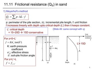
1) Meyerhof’s method
Qs  pL f
p: perimeter of the pile section, L: incremental pile length, f: unit friction
f increases linearly with depth upto critical depth (L’) then it keeps constant.
'

o
f  K tan( )
For z=0~L’
L’: critical depth
= 15~20D  15D conservative
K: earth pressure
coefficient
’o: effective stress
’: soil-pile friction angle
For z=L’~L
f  fzL'
(Slide 49: same concept with q)

2. K: Effective earth coefficient
2
Pile type K
Bored or jetted K ? Ko 1- sin'
Low-displacement (open ended) K ? (1~1.4)Ko (1~1.4)(1- sin')
High-displacement (closed ended) K ? (1~1.8)Ko (1~1.8)(1- sin')
’: friction angle between soil and pile
Pile material ’
Steel ’=(0.67~0.83)’
Concrete ’=(0.9~1.0)’
Timber ’=(0.8~1.0)’
11.11 Frictional resistance (QS) in sand

3. K  0.93
@ L / D  33.3,  35o
2) Coyle and Castello’s method
Data from 24 large scale field tests
of driven piles in sand
11.11 Frictional resistance (QS) in sand
o : Average effective
overburden pressure
’=0.8’: soil-pile friction angle
K: lateral earth pressure
coefficient  f(L/D, ’)
QS  fav pL  (Ko tan)pL
 Ko tan(0.8')pL
3

4. Example 11.5
Part a: Meyerhof’s method
1) Critical Depth L 15D  (15)(0.45)  6.75m
0
'
 0
f  0
For Z=0 to L’ For Z= L’ to L
f  fzL'
At z = 6.75m
At z = 0m
'
 )

o
f  K tan(
L’= 15D
D=0.45m
• A concrete pile is 15m(L) long and 0.45mX0.45m in cross section.
The pile is fully embedded in sand for which =17kN/m³ and ’=35˚.
Calculate the ultimate skin friction, Qs
– a. Meyerhof’s method: Use K=1.3 and '
 0.8'
– B. The method of Coyle and Castello.
 (6.75)(17) 114.75kN / m2
0
'
'
 79.3kN / m2
o

f  K tan( )  (1.3)(114.75)[tan(0.835)]
4

5. Example 11.5
2
2
 

 
  0  79.3(4 0.45)(6.75)  (79.3)(4 0.45)(15 6.75)
 
 
z0 z6.75m
s  z6.75m
f  f
Q  pL' f p(L  L')
L’= 15D
2) Ultimate skin friction, Qs
Part b: Coyle and Castello’s method
 481.751177.61 1659.36kN  1659kN
Part b: Coyle and Castello’s method
QS  Ko tan(0.8')pL
 K  0.93
Qs  (0.93)(127.5) tan[(0.835)](40.45)(15) 1702kN
2
L/ D 15/0.45  33.3;   35
o 
(15)(17)
 127.5kN / m2
5

6. Part c: Using the results of Part d of Example 11.1,
estimate the allowable bearing capacity of the pile (Use FS=3)
Average value of Qs from part a and b
Example 11.5

1250 1680
 977kN
3

Qp  Qs
all
Q
FS
From part d of Example 11.1, Qp=1250kN
2
6
s(average)
Q 
1659 1702
1680.5 1680kN

7. 3) Correlation with SPT (Meyerhof)
fav (kN /m2
) = 2(N60)
fav (t /m2
) = 0.2(N60)
High displacement driven pile
Low displacement driven pile
Qs  pLfav
11.11 Frictional resistance (QS) in sand
fav (kN / m2
) = 1(N60)
fav (t / m2
) = 0.1(N60)
(N60) : the average of SPT N-value
MRT: 0.3N
7

8. Example 11.4
Depth below
ground
surface (m)
N60
1.5 8
3.0 10
4.5 9
6.0 12
7.5 14
9.0 18
10.5 11
12.0 17
13.5 20
15.0 28
16.5 29
18.0 32
19.5 30
21.0 27
Refer to the pile describe in Example 11.3.
Concrete pile, L=15.2m,A=305mmX305mm.
Q: Estimate the magnitude of Qs for pile.
High displacement driven pile
fav (kN / m2
) = 2(N60)
= 8+ 10+ 9+ 12+ 14+ 18+ 11+ 17+ 20+ 28 = 14.7 ? 15
N60
10
Qs  pLfav  (4 0.305)(15.2)(30)  556.2kN
Allowable load-carrying capacity (Use FS=3)

893 556.2
 483kN
3

Qp  Qs
all
Q
FS
av
f  2(N60 )  (2)(15)  30kN / m2
8

9. f =  'fc Qs  pL f  pL ' fc
11.11 Frictional resistance (QS) in sand
4) Correlation with CPT
’ for electric cone penetrometer
9
’ for mechanical cone penetrometer
'  0.44
@ z / D  16
f: unit skin friction; fc: frictional resistance (CPT)

10. Concrete pile: 305mmX305mm, L=18m
Fully embedded in a sandy soil
CPT (mechanical cone results)
Q: Estimate the allowable load (Use FS=3)
Qp = Apqc = (0.305*0.305)(9500) = 883.7kN
2) Skin friction
L/D
= 5/0.305
= 16
(kN/m ) (kN/m )
Example 11.6 Depth from
ground
qc
2
fc
2
surface (m)
0-5 3040 73
5-15 4560 102
15-25 9500 226
1) End bearing: qp  qc (in granular soils: Meyerhof)
Qs 1107.35kN
3) Ultimate and allowable loads
Qu  Qp Qs  883.71107.35 1991.05kN
3

Qu
all
Q
FS

1991.05
 663.68  664kN
Depth from ground
surface (m)
△L
(m)
fc (kN/m2
) α
' p
p△Lα'fc
(kN)
0-5 5 73 0.44 4*0.305 195.9
5-15 10 102 0.44 1.22 547.5
15-25 3 226 0.44 1.22 363.95
10

11. 11.12 Frictional (Skin) resistance in Clay
11
• Clay  QP is small  QS is important
– , ,  methods
 method: total stress + effective stress
 method: total stress
 method: effective stress
– Correlation with CPT

12. 1)  method: total stress + effective stress
• Suggested by Vijayvergiya & Focht (1972)
– Based on the assumption that the
displacement of soil casued by pile
driving results in a passive lateral
pressure at any depth
• Average unit skin resistance
 depends on the penetration depth
Average skin resistance
fav  (o
  2cu )
11.12 Frictional (Skin) resistance in Clay
QS  pLfav
 0.136
@ L  30m
12

13. • Average unit skin resistance
– cu =(L1cu1+L2cu2+L3cu3+․․․)/L : mean undrained shear strength
1 2 3
=(A +A +A +․․․ )/L : mean vertical effective stress
for the entire embedment depth
1)  method: total stress + effective stress
o
–  ¢
11.12 Frictional (Skin) resistance in Clay
fav  (o
  2cu )
13

14. 1
11.12 Frictional resistance in Clay
Qs = 檍fpL = cupL
f = cu
2)  method: total stress
• Suggested by Tomlinson
• Unit skin friction
念
¢ 0.45
o
÷
 = Cç
ç
曜
cu ÷
: empirical adhesion factor
C  0.4~0.5: bored piles
C  0.5: driven piles
Soft:  = 1
Stiff:  < 1
Table 11.10
4

15. 11.12 Frictional resistance in Clay
QS = å fpL
3)  method: effective stress
• Suggested by Burland(1973)
• Pile driving in saturated clay  Generation of excess pore water pressure
 Dissipation  effective stress
f  'o
σ’0= vertical effective stress β
= K tan’R
’R =drained friction angle of remolded clay
K = earth pressure coefficient
'
'
= (1- sin )
= (1- sin )
R
R
NC clay K
OC clay K OCR
OCR: overconsolidation ratio
15

16. 11.12 Frictional resistance in Clay
4) Correlation with CPT
• Suggested by Schmertmann (1975)
f: unit skin friction
fc: frictional resistance (CPT)
16
Qs  pL f  pL' fc
f = 'fc
f =  'fc
Qs  pL f  pL' fc
Same equation in sand and clay
But ' is pretty much different

17. Example 11.7
17
Top 10m: NC clay
Bottom: OC clay (OCR=2)
A driven pipe pile in clay
OD=406mm
p  (0.406)  1.275m
Q: Calculate the skin resistance
By 1)  method; 2)  method; 3)  method (’R=30o)
1)  method: total stress Qs = 檍fpL= cupL
Depth from ground
surface (m)
△L(m) Cu(kN/m2
) Cu/Pa  αCup△L(kN)
0-5 5 30 0.3 0.82 156.83
5-10 5 30 0.3 0.82 156.83
10-30 20 100 1.0 0.48 1224.0
Qs=1538kN

18. Example 11.7
fav  (o
  2cu )
2)  method: total stress + effective stress
30
u
c 
cu(1)L1  cu(2)L2  cu(3)L2

(30)(5)  (30)(5)  (100)(20)
 76.7kN /m2
30
A1 A2  A3
 ' 
o
L

225 552.38 4577
 178.48kN / m2
30
2
av o u
f  (  2c )  0.136(178.48 2 76.7)  45.14kN / m
QS  pLfav 
(0.406)(30)(45.14) 1727kN
18

19. Example 11.7
3)  method: effective stress
'
'
R
R OCR
- sin )
- sin )
NC : K = (1
OC : K = (1
' ' '
o R o
f =  = K tan 
' ' '
2
R R o
0~5m: fav(1) = (1- sin )tan  = (1- sin30)(tan30)(
0+ 90
) = 13.0kN / m2
2
5~10m : fav(2) = (1- sin30)(tan30)(
90 +130.95
) = 31.9kN / m2
2
19
10~20m : fav(3) = (1- sin30) 2(tan30)(
130.95+ 326.75
) = 93.43kN / m2
Qs = p[ fav(1)(5)+ fav(2)(5)+ fav(3)(20)]
= ()(0.406)[(13)(5)+(31.9)(5) +(93.43)(20)] = 2670kN
QS = å fpL

20. Example 11.7
b. Estimate the net allowable pile capacity (FS=4).
1) End bearing
Qp  133 kN (Ex 11.2)
2) Skin friction
Qs(  method )  1538kN Qs(  method)  1727kN
Qs(average) 
1538 1727
 1632.5kN
2
3) Ultimate capacity
Qu = Qp + Qs = 133+ 1632.5 = 1765.5kN
4)Allowable capacity
Qall =
Qu
=
1765.5
? 441kN
Fs 4
20
Qs(  method)  2670kN

21. Example 11.8
21
Concrete pile: 305mmX305mm, L=20m,
Saturated clay. CPT: fc
Q: Estimate the frictional resistance Qs
Correlation with CPT
f =  ' fc
Depth (m) fc (kN/m2) fc /Pa α
' △L (m) p△L α'fc (kN)
0-6 34.34 0.34 0.84 6 211.5
6-12 54.94 0.55 0.71 6 285.5
12-20 70.63 0.70 0.63 8 434.2
* p = (4)(0.305)=1.22m Qs   pL ' fc  931kN

22. 11.13 Point bearing capacity of piles resting on rock
Ultimate unit point resistance
qu (lab )
22
qp = qu (N + 1)
N = tan2
(45+ '/ 2)
qu: unconfined compression strength of rock
’ : drained friction angle

23. 11.13 Point bearing capacity of piles resting on rock
Allowable load
u(lab)
5
u(design)
q
=
q QP(all) =
[qu(design) (N + 1)]Ap
FS
Scale effect
Scale effect
Ap: NetArea
(not plug part)
REV: Representative Elementary Volume
permeability
23
strength
Lab Field

24. Example: QP on Rock
Area of H-Pile (Net Area)  Table 11.1.
: HP 310X125piles: Ap=15.9X10-3 m2

2
5 2
28
5 2
3 2
182kN
5

76 103
kN / m2
 
tan (45 
FS
qu(lab)  tan2
(45 
'
)  1
Ap

 

 


Qp(all )  

) 1 15.910 m 
 
  
 

 
H-pile(310X125, L=26m) is driven through a soft clay layer to rest on
sandstone. Sandstone: qu(lab) = 76MN/m², ’ = 28˚.
Q: Estimate the allowable point bearing capacity (FS=5)
u(lab)
5
u(design)
q
=
q
QP(all) =
[qu(design) (N + 1)]Ap
FS
N = tan2
(45+  '/ 2)
24

25. Ch 11. Pile foundations
25
• Contents
1. Introduction
2. Types of piles and their structural characteristics
11.4 Installation of piles
11.3 Estimating pile length
5. Load transfer mechanism
6. Equations for estimating pile capacity
– QP: 11.7~ 11.10
– QS: 11.11~11.12
– Pile bearing capacity on rock: 11.13
14. Pile load tests
15. Elastic settlement of piles
16. Laterally loaded piles

26. 26
11.14 Pile Load Tests (Compression test)
Dead weight = Kentledge method

27. 27
11.14 Pile Load Tests (Compression test)

28. 28
11.14 Pile Load Tests (Compression test)

29. 9
2
Tension pile
11.14 Pile Load Tests (Compression test)

30. 30
11.14 Pile Load Test (Compression test)
Tension pile

31. 31
11.14 Pile Load Test (Compression test)
Anchor

32. 32
11.14 Pile Load Test (Compression test)
Anchor

33. 11.14 Pile Load Tests (Compression test)
Test procedure
1. ML (Maintained Load): load is sustained at each level until all
settlement has either stop or does not exceed a specified amount.
• SM: Slow Maintained Load Test  0.025mm/hr
• QM : Quick Maintained Load Test  2.5-15 minutes/step
• At least twice of the design load (200%)
• At least 8 load steps (25% of design load at each step)
2. CRP (Constant Rate Penetration): load is adjusted to give constant
rate of downward movement of the pile until it reaches the failure.
* Failure: downward pile movement without increasing load,
penetration of one-tenth of the diameter of the pile at the base
33

34. 34
11.14 Pile Load Tests (Compression test)
Test results
1) Load-time
2) Load-settlement

35. 11.14 Pile Load Test (Compression test)
Test results
2) Load-settlement
Qy: Yield load
: curvature of load – settlement
curve becomes maximum
Qu: Ultimate load
: load-settlement curve
becomes vertical
Settlement
Load
Qu: Ultimate load
35
Qy: Yield load

36. 11.14 Pile Load Test (Compression test)
Disturbance due to pile driving
Remolded or compacted zone around a pile driven into soft clay
Variation of undrained shear
strength (cu) with time around
a pile driven into soft clay
30~60days
36

37. 11.14 Pile Load Test (Compression test)
Time effects
Variation of Qs and Qp with
time for a pile driven
Setup (or freeze): capacity increase with time after installing driven piles.
Setup occurs in saturated clays and silts due to the dissipation of excess
pore pressure at the skin friction.
Relaxation: capacity decrease with time after installing driven piles.
Relaxation occurs in dense fine sand or stiff fissured clay at the pile tip.
37

38. 11.14 Pile Load Test (Tension or Pullout test)
• Tension, Pullout, uplift
• ML (Maintained load) or CRU (Constant rate of uplift)
• This test method was discontinued in 2003 by ASTM
38

39. 11.14 Pile Load Test (Compression test)
39

40. 11.14 Pile Load Test (Lateral loading test)
• This test method was discontinued in 2003 by ASTM
Pair of piles
(Reaction pile)
Single pile
(Kentledge weight)
40

41. 41
11.14 Pile Load Tests (Compression test)
u r
p p
A E
s (mm)  0.012D  0
 D 

QuL
.1 D 
 r  QuL
ApEp
r
 D 
0.012D  0.1 D 
 r 
Qu (kN): ultimate load
D(mm): Diameter or width
Dr: reference diameter or width (300mm)
L(mm): pile length
Ap(mm2): cross sectional area
Ep(kN/mm2): Young’s modulus of pile
Ultimate load by Davisson’s method
Settlement for ultimate load Qu
u
p p
s (mm)  3.81
D(mm)

QuL
D  609.6mm
120 A E
u
p p
s (mm)  3.81
D(mm)

QuL
D  609.6mm
30 A E
1) Original
2) Simplified (Design Code)

42. Example 11.9
Figure shows the load test results of a 20m long concrete pile (406mm x
406mm) embedded in sand. (Ep = 30 x 106 kN/m2)
Q: Using Davisson’s method, determine the ultimate load Qu
u r
1) Settlement for Qu s
 D 

QuL
 0.012D  0.1 D 
 r  p p
A E
2) Dr=300mm, D=406mm, L=20,000mm
Ap=164,836mm2, Ep=30x106kN/m2
(30)(164,836)
u
 406  
Qu (20,000)
s  (0.012)(300)  0.1 300 
 
 3.6  0.135  0.004Qu
 3.735  0.004Qu
3) The intersection of this line with the load-
settlement curve gives the failure load
Qu =1460kN
42

43. 11.15 Elastic settlement of piles
43
The total settlement of a pile under a vertical working load Qw
se = se(1) + se(2) + se(3)
se(1) = axial deformation of pile
se(2) = pile settlement due to load at pile tip
se(3) = pile settlement due to load along pile shaft

44. Se(1) =
(Qwp +Qws)L
ApEp
11.15 Elastic settlement of piles
Qwp= load carried at the pile point under
working load condition
Qws= load carried by frictional (skin)
resistance under working load condition
Ap = area of cross section of pile
L = lengh of pile
Ep= modulus of elasticity of the pile material
1) se(1) : axial deformation of pile
QwpL
ApEp
44

45. 11.15 Elastic settlement of piles
** same method discussed in shallow foundation
D : width or diameter of pile
qwp (=Qwp/Ap) : point load per unit area at the pile point
Qwp : load carried at the pile point under working load condition
Es : modulus of elasticity of soil at or below the pile point
s : Poisson’s ratio of soil
Iwp : influence factor ≈ 0.85
Es
Se(2) 
qwpD
(1 s
2
)Iwp
Soil type Driven pile Bored pile
Sand 0.02 ~ 0.04 0.09 ~ 0.18
Clay 0.02 ~ 0.03 0.03 ~ 0.06
Silt 0.03 ~ 0.05 0.09 ~ 0.12
S =
QwpCp
Dqp
e(2)
Vesic’s semi-empirical method Table 11.13
45
Typical values of CP
2) se(2) : pile settlement due to load at pile tip
qp : ultimate point load of the pile
Cp: empirical coefficient
(sec 5.10: simple method
 rigid foundation)

46. 11.15 Elastic settlement of piles
p = perimeter of the pile
L= embedded length of pile
Qws/pL : average value of f along the pile shaft
Iws= influence factor
s
pL E
  
  
Se(3) 
Qws  D (1 s
2
)Iws
e(3)
p
S =
QwsCs
Lq
Iws = 2+0.35
L
D
Vesic’s semi-empirical method
CS = empirical constant
CS = (
0.93+ 0.16 L/ D)
CP
46
3) se(3) : pile settlement due to load along pile shaft
Soil type Driven pile Bored pile
Sand 0.02 ~ 0.04 0.09 ~ 0.18
Clay 0.02 ~ 0.03 0.03 ~ 0.06
Silt 0.03 ~ 0.05 0.09 ~ 0.12
Table 11.13 Typical values of CP

47. The allowable working load on a prestressed concrete pile 21-m long that
has been driven into sand is 502kN. The pile is octagonal in shape with D =
356mm. Skin resistance carries 350kN of the allowable load, and point
bearing carries the rest.
(use Ep = 21 x 106kN/m2, Es=25x103kN/m2, s=0.35, and =0.62 )
Q: Determine the settlement of the pile
1) se(1) : axial deformation of pile
 502  350  152kN
e(1)
(0.1045m2
)(21106
)

[152 0.62(350)](21)
 0.00353m  3.53mm
S
Example 11.10
Se(1) =
(Qwp +Qws)L
ApEp
Octagonal pile with D=356mm
From Table 11.3a : Ap=1045cm2, p=1.168m
Skin friction: QWS=350kN  End bearing: QWp
47

48. 2
3
152
s WP
s
qWPD
E
Se(2)  (1  )I
   0.356 
1 0.352
(0.85)  0.0155m  15.5mm
  
0.1045 2510
  
s
pL E
  
  
Se(3) 
Qws  D (1 s
2
)Iws
  




 350
3
 0.356 (1 0.352
)(4.69)  0.00084m  0.84mm
(1.168)(21) 2510
 4.69
0.356
21
D
I  2  0.35
L
 2  0.35
WS
4) Total settlement :
se  se(1)  se(2)  se(3)  3.5315.5 0.84 19.96mm
2) se(2) : pile settlement due to load at pile tip
3) se(3) : pile settlement due to load along pile shaft
Example 11.10
48

49. Ch 11. Pile foundations
49
• Contents
17. Pile driving formulas
18. Pile capacity for vibration-driven piles
19. Negative skin friction
Group piles
20. Group efficiency
21. Ultimate capacity of group piles in saturated clay
22. Elastic settlement of group piles
23. Consolidation settlement of group piles
24. Piles in rock

50. 11.17 Pile-driving formulas
So: Set value So
Energy conservation: E(pile impact) = W(for penetration)+W(lost)
Spp : plastic deformation of pile
50
Sep : elastic deformation of pile
Ses : elastic deformation of soil

51. 11.20 Pile-driving formulas
Qu 
WRh
S C
1) Engineering News Record (ENR) formula – Ultimate capacity
WR = weight of the ram
h = height of fall of the ram
S = penetration of the pile per hammer blow
C = 2.54mm (steam hammer) ~ 25.4mm (drop hammer)
2) Based on Hammer efficiency
Qu =
EHE
S + C
EWRh 念
WR + n2
Wp ÷
Qu = ç ÷
÷
S + C ç
曜
ç WR + W p
3) Modified ENR formula
S: set value (mm/blow)
n: coefficient of restitution (0.25 ~ 0.5)
51
P
W : weight of pile including cap
E : hammer efficiency
HE : rated energy of the hammer

52. 11.20 Pile-driving formulas
4) Danish formula
E
52
u
EH
EHE L
2Ap Ep
S 
Q 
E : hammer efficiency
HE : rated energy of the hammer
EP: elastic modulus of pile
S: set value (mm/blow)
L: pile length
AP: cross-sectional area of pile
5)Allowable bearing capacity: Qall = Qu/ FS

53. A precast concrete pile 0.305m x 0.305m in cross section is driven by
hammer.
- Maximum rated hammer energy = 40.67kN-m
- Weight of ram = 33.36kN
- Coefficient of restitution(n) = 0.4
- Hammer efficiency = 0.8
- Pile length = 24.39m
- Weight of pile cap = 2.45kN - Ep = 20.7 x 106kN/m2
- Number of blows for last 25.4mm of penetration = 8
Q: Estimate the allowable pile capacity by the modified ENR formula (FS = 6)
2) Ultimate load (Qu) :
25.4
8
(0.8)(40.671000)  33.36  (0.4)2
(55.95) 

EW h W  n2
W

Qu  R
 R P

S  C  WR WP
   2697kN
33.36  55.95
 
 2.54

 55.95kN
P
1) Weight of pile +cap W  (0.305  0.305  24.39)(23.58kN /m3
)  2.45
Example 11.14
6

2697
 449.5kN

Qu
all
Q
FS
Unit weight
53

54. A precast concrete pile 0.305m x 0.305m in cross section is driven by
hammer.
- Maximum rated hammer energy = 40.67kN-m
- Weight of ram = 33.36kN
- Coefficient of restitution(n) = 0.4
- Hammer efficiency = 0.8
- Pile length = 24.39m
- Weight of pile cap = 2.45kN - Ep = 20.7 x 106kN/m2
- Number of blows for last 25.4mm of penetration = 8
Q: Estimate the allowable pile capacity by the Danish formula (FS = 4)
Example 11.14
(0.8)(40.67)
 1857kN
 0.01435
u
EHE
EH L
E
2ApEp
Q 
S 
25.4
8 1000

(0.8)(40.67)(24.39)
2(0.305 0.305)(20.7 106
)
 0.01435m  14.35mm
p p
2A E
EHEL

4

1857
 464kN

Qu
all
Q
FS
54

55. 11.19 Negative skin friction
Negative skin friction = downward drag force
Settlement of soils is greater than that of pile.
1. After a pile is driven, a clay soil is placed over a granular soil 
consolidation
2. A granular soil is placed over a soft clay  consolidation
3. Lowering of water table  increase in effective stress  consolidation
L1
55

56. 11.19 Negative skin friction
Load transfer mechanism
56

57. 11.19 Negative skin friction
K'=Ko=1-sin’ : earth pressure coefficient
o’ = f
’ z: vertical effective stress
f
’ : effective unit weight of fill
’ =(0.5 ~ 0.7)’ : soil-pile friction angle
Hf : height of fill
0 0
0
H f H f
H f
o 'dz
pK ' tan
f
pK '¢z tan'dz
¢
Qn = 窒 pfndz =
= ò
n o
¢
f = K ' tan '
1) Clay fill over granular soil
 Similar to -method
Unit negative skin friction
1
2
tan '
f
2
f
¢
Qn = pK ' H
57

58. Example 11.16
H = 2m. Pipe pile (D=0.305 m, ’ = 0.6 ). Clay
fill (above the water table),  = 16 kN/m3,  = 32.
Q: Determine the total drag force
p = (0.305) = 0.958m
K ' = 1- sin '= 1- sin 32 = 0.47
 '  (0.6)(32)  19.2
n
Q =
1
(0.958)(0.47)(16)(2)2
tan19.2
2
= 5.02 kN
1
2
tan '
f
2
f
¢
Qn = pK ' H
58

59. 1
2
n f f 1
Q = (pK '¢H tan')L +
1
pK ''L2
tan'
11.19 Negative skin friction
 End bearing pile: L1 = L-Hf
 Friction pile (Bowles, 1982)
 Unit negative skin friction
1
1 2  '
f f f f
 '
f f
 H 2 H
L
念 ⇔
(L- H ) L- H
÷
L = + -
ç
÷
ç
曜
2) Granular soil fill over clay
Negative skin friction: 0~L1 (neutral depth)
 Direction change in skin friction
'
n o
f = K ' tan '
L1
0
L1
0
+  ' z)tan 'dz
Qn = 窒pfndz = f f
pK '( H
¢
K'=Ko=1-sin’
’ =(0.5 ~ 0.7)’
f
 ¢
 '
L1
59

60. 60
Example 11.17
Pile: OD= 0.305m, L = 20m, ’ = 0.6clay.
Sand fill: H = 2m,  = 16.5 kN/m3
Clay: clay = 34, sat(clay) = 17.2kN/m3
Water table = top of the clay layer.
Q: Determine the downward drag force.
Depth of neutral plane
1
1  '  '
f f f f f f
 H 2 H
L
念 ⇔
L- H L- H ÷
L = + -
ç ÷
÷
ç
曜 2
(2)(16.5)(2)
(16.5)(2) 

1 
  
2 (17.2 9.81) (17.2 9.81)
20  2  20  2
L1 
L 
? L1 11.75m
Sand

Clay
clay
sat(clay)
1
1
L
L =
242.4
- 8.93
p  (0.305)  0.958m
∘
K'1sin 34  0.44
 ' = (0.6)(34) = 20.4
Qn = (0.958)(0.44)(16.5)(2)[tan(20.4)](11.75)
(0.958)(0.44)(17.2- 9.81)(11.75)2
[tan(20.4)]
+
2
= 60.78+ 79.97 = 140.75kN
L1
1
2
n f f 1
Q = (pK '¢H tan')L +
1
pK ''L2
tan'

61. Ch 11. Pile foundations
61
• Contents
17. Pile driving formulas
18. Pile capacity for vibration-driven piles
19. Negative skin friction
Group piles
20. Group efficiency
21. Ultimate capacity of group piles in saturated clay
22. Elastic settlement of group piles
23. Consolidation settlement of group piles
24. Piles in rock

62. 11.20 Group efficiency
Pile spacing Pile action
< (3 ~ 7)D Group
> 7D Individual
62
Group pile or single pile ?

63. 11.20 Group efficiency
63

64. • Group piles
1) Bearing capacity of group piles is
extremely complicated and has
not yet been fully understood
2) Different group action of friction
piles and end-bearing piles
3) Effects of pile cap
11.20 Group efficiency
Group effect is
greater when cap
is on the ground
Capacity
decreases
Capacity
shouldn’t be
decreased
64

65. 11.20 Group efficiency
Efficiency of load-bearing capacity of a group pile
 
Qg(u)
Qu
 = group efficiency
Qg(u) = ultimate load-bearing capacity of
the group pile
Qu = ultimate load-bearing capacity of
each pile without the group effect
65

66. 11.20 Group efficiency
(1) Frictional capacity
when acting as a block
p: perimeter of each pile
Group efficiency
<1.0: Qg(u) = η
Σ
Q
u
>1.0: Qg(u) = ΣQu
Capacity
1) Group efficiency of friction piles
66
Qu = fav pL
av g g
殞
Qg(u) ? fav pg L f 2(L + B ) L
薏
= fav [
2(n1 + n2 - 2)d + 4D]
L
pg=2(n1+n2 - 2)+4D: perimeter of block
(2) Frictional capacity
when acting individually

67. Name Equation
Converse-Labarre
equation
Los Angeles Group
Action equation
Seiler-Keeney
equation
2) Other equations for group efficiency of friction piles
11.20 Group efficiency
67

68. 11.20 Group efficiency
3) Group efficiency of friction piles – empirical method
Ultimate capacity is reduced by 1/16 by each adjacent diagonal or row pile
Pile
type
Pile
No.
No of
adjacent pile
Reduction
factor
Ultimate capacity
A 1 8 1-8/16 1×Qu×(1-8/16) = 0.5Qu
B 4 5 1-5/16 4×Qu×(1-5/16) = 2.75Qu
C 4 3 1-3/16 4×Qu×(1-3/16) = 3.25Qu
Qg(u) = (0.5+2.75+3.25)Qu = 6.5Qu
Group efficiency
9
68
 
6.5
 72%

69. 11.20 Group efficiency
4) Bearing capacity of group piles in Sands
Pile spacing:
CTC (center-to-center) > 3D
(1) End bearing of group pile
Qg(p) = nQp
n: pile no.
Qp: ultimate end bearing of
each pile
(2) Skin friction of group pile
Qg(s) ≥ ΣQs
due to compaction & lateral
compression (for loose sand)
(3) General: ≥1.0
69

70. 11.20 Group efficiency
5) Bearing capacity evaluation of group piles in sands
1) CTC > 3D
Qg(u) = ΣQu= Σ(Qp + Qs)
2)Weak layer in pile tip
smaller value from (1) and (2)
(1) Summation of individual piles
Qg(u)1=nΣQu=nΣ(Qp + Qs)
(2) Capacity of block failure
Qg(u)2 = Qg(s) + Qg(p)
Qg(s) = 2(Bg+Lg)fav(g)L
Qg(p) = End bearing of weak layer
(Bg×Lg)
3) Bored pile groups with d (CTC)≒3D
Qg(u) = (⅔～¾)ΣQu
= (⅔～¾)Σ(Qp+ Qs)
70

71. 7
Qg(u)  Qu  n1n2 QP QS 
 n1n2 9Apcu( p)  cu pL
11.21 Ultimate capacity of group piles in saturated clay
The lower value from (1) and (2) is is Qg(u)
(1) Summation of individual pile
g g u( p) c
(2) Capacity of block failure
Qg(u)  Qg(P)  Qg(S)
 L B c N
2(Lg  Bg )cuL
1

72. 72
Upper layer:  1  0.68
cu(1) / Pa  50.3/100  0.503
Example 11.18
34 Group pile
Square pile: 356  356mm
Center-to-center spacing: 889mm
Saturated clay
Ground water table: ground surface
Q:Allowable load-bearing capacity
of the pile group (FS=4)
(1) Summation of individual pile
Qg(u)  n1n2 9Apcu( p)
 n1n2 9Apcu( p) 1cu(1) pL1 2cu(2) pL2 
 cu pL
Lower layer: cu(2) / Pa  85.1/100  0.851  2  0.51
u
9(0.356)2
(85.1)  (0.68)(50.3)(4 0.356)(4.57)
Q  (3)(4)  
(0.51)(85.1)(40.356)(13.72)
 
14,011kN

73. Lg  (3)(0.889)  0.356  3.023m
Bg  (2)(0.889)  0.356  2.134m
Example 11.18
(2) Block failure
g(u) g g u( p) c
Q  L B c N
2(Lg  Bg )cuL

3.023
1.42,
L

18.29
 8.57  8.75

Lg
c
N
g
B 2.134 g
B 2.134

14,011

14,011
 3,503kN
FS 4
73
all
Q
g(u) g g u( p) c g g u
Q  L B c N
 2(L  B )c L
 (3.023)(2.134)(85.1)(8.75)  (2)(3.023 2.134)(50.3)(4.57)  (85.1)(13.72)
 19,217kN
(3) Lower value Qu  14,011kN
(4)Allowable load-bearing capacity

74. 11.22 Elastic settlement of group piles
Settlement of group piles (sg) is greater than settlement of single pile (s)
at equal load per pile
Sg increases with the width of group
pile (Bg) and CTC spacing of piles (d)
(Meyerhof, 1961), D: pile diameter
74

75. g(e) e
S
Bg
D
S =
1) Vesic (1977)
q=Qg/(LgBg) in kN/m2
Lg & Bg = length and width of pile group section (m)
N60 =average corrected SPT N-value
within seat of settlement ( Bg deep below pile tip)
I=influence factor = 1-L/(8Bg) ≥ 0.5
L= length of embedment of piles (m)
Sg(e) = elastic settlement of group piles
Bg = width of group pile section
D = width or diameter of each pile in the group
Se= elastic settlement of each pile
at comparable working load
2) Meyerhof(1976)
60
75
0.96q Bg I
N
Sg(e)(mm) =
11.22 Elastic settlement of group piles

76. 3) CPT correlation g
76
g(e)
c
qB I
2q
S =
11.22 Elastic settlement of group piles
q=Qg/(LgBg) in kN/m2
Lg & Bg = length and width of pile group section (m)
I=influence factor = 1-L/(8Bg) ≥ 0.5
L= length of embedment of piles (m)
qc = average cone penetration resistance
within the seat of settlement

77. g
B  (31)d  2 D   (2)(3D)  D  7D  (7)(0.356m)  2.492m
 2 
 
0.356
e(g)
S 
2.492
(19.69)  52.09mm
34 Group pile
Octagonal pile: D=356mm
Center-to-center spacing: 3D
Pile length L=21m
Sandy soils
Details of each pile and the sand are described in Example 11.10
Working load of group pile = 6024kN:  34Qall = 6024kN  Qall = 502kN
Q: Estimate the elastic settlement of the pile group by Vesic method
1) Settlement of single pile (Example 11.10) se  19.96mm
g(e)
Bg
e
S = S
D
2) Vesic method
Example 11.19
77

78. 11.23 Consolidation settlement of group piles
oi
 ¢
2) Assume that Qg is transmitted at (2/3)L from top.
Load spreading  2:1 (2V:1H)
3) Effective stress increase at the middle of clay layer
Qg
i
Qg
¢=
(Bg + zi )(Lg + zi )
i
 ¢
i
g i g i
Qg
¢=
(B + z )(L + z )
z
1) Total load
Qg = Load from superstructure – effective weight of soil removed
2/3L
78
2/3L
L

79. 11.23 Consolidation settlement of group piles
4) Disregard the settlement above (2/3)L
5) Settlement below (2/3)L
log oi
oi
Hi 
念 ⇔
+ i ÷
S = çCci ÷
÷
¢
1+eo i
ç
曜
ci å
i
oi i
ci si ci
i oi pi


Hi
念 ¢ ⇔
+  ÷
çC log pi
+ C log ÷
⇔ ÷
1+ e ç
oi 曜
S = å
NC clay
79
OC clay
6) Total settlement Sg = å Sci

80. A group pile in NC clay
Q: Determine the consolidation
settlement of the piles
L=15m
2:1 distribution starts at 10m
Qg = 2000kN
0(1) (1)
0(1) 0(1)
log
c(1) 1
c(1)
C H
殞 殞
 ' + '
油 油
S =
油
1 + e 油  '
薏 薏
'0(1)  2(16.2) 12.5(18.0 9.81) 134.8kN / m 2
Example 11.20
Clay layer 1
= 51.6kN / m2
(1)
g 1 g 1
2000
 ' =
Qg
=
(L + z )(B + z ) (3.3+ 3.5)(2.2+ 3.5)
(0.3)(7) 殞
134.8+ 51.6
Sc(1) = log 油 = 0.1624m = 162.4mm
1+0.82 油
薏 134.8
Clay1
80
Clay2
Clay3

81. (2)
0(2)  '0(2)
殞
 ' + '
log 油 0(2)
H
殞
C
Sc(2) = 油
c(2) 2
油
1+ e 油
油
薏 油
薏
2
2000
'(2) 
(3.39)(2.29)
14.52kN / m
Sc(2) =
(0.2)(4)
= 0.0157m = 15.7mm
1+ 0.7 181.62
殞
181.62+ 14.52
log 油
油
薏
Clay layer 2
o(2)
 ' = 2(16.2)+16(18.0- 9.81)+2(18.9- 9.81)= 181.62kN / m2
(3)
 ' =
2000
= 9.2kN / m2
(3.3+ 12)(2.2+ 12)
Total settlement
Sc(g) = 162.4+ 15.7+ 5.4 = 183.5mm
Clay layer 3
S(3) =
(0.25)(2) 殞
208.99+ 9.2
log 油 = 0.0054m = 5.4mm
1+0.75 油
薏 208.99
2
 '0(3) = 181.62+2(18.9- 9.81)+1(19- 9.81)= 208.99kN / m
Example 11.20
(3)
c(3)
0(3)
 '
殞
C H3 殞
 ' + '
log 油 0(3)
= 油c(3)
S 油
油
1 + e
薏
油 0(3) 油
薏
81

82. 11.24 Bearing capacity of group piles in rock
Point bearing group piles
82
if d  D  300mm
Qg(u)  Qu

83. • Assignment # 11-1 (Capacity)
– Due: Next Week
– Problems: 11.1 ~ 11.5 // 11.10, 11.11
• Assignment # 11-2 (Settlement)
– Due: (Saturday)
– Problems: 11.13 // 11.16~11.18 // 11.20, 11.21
• Assignment # 11-3 (Group pile)
– Due: (Saturday)
– Problems: 11.23, 11.25 // 11.26
83
Homework Assignment - Chapter 11

84. 3rd Exam
December 10 (Saturday) 10:00 ~ 13:00
Chapter 6 & 11
Closed book
Calculator
No Smart Devices
84
Announcement

85. Weight Remarks
Attendance &
Participation
15%
The student should attend more than 3/4 of the
classes scheduled.
Personal meeting.
Homework
Assignments
20%
Homework will be given weekly (or biweekly
depending on the topics).
It should be handed in a week after the date assigned.
Examinations 70%
1st Option: 70/3=23.3% each
2nd Option: 15%, 20%, 35%
 Grade is based on the better one.
85
Grading

86. 86
Setup
ASTM D 4945
Pile Driving Analyzer (PDA)

87. Wave propagation in pile (1D)
• Smith Model (1960)
– Pile : lumped mass
spring
– Soil : viscoelastic-plastic
• 1D wave Equation
R
2
u

E 2
u

t2
 x2
87

88. Proportionality
• Wave speed
• Strain
• Rearrangement
• EA 



E 

L 
c 
t

L t c
 
 

t
• Particle Velocity V 

c
F 
EA
V  ZV
c
88
 
V

89. • Piles driven to rock
– Notes
– H형 강말뚝, 강관말뚝, 콘크리트 말뚝과 암반간의 정확한 접촉면적 산정 어려움
– 지지력은 암석의 종류와 특성, 말뚝의 암석내 근입깊이 등에 좌우
– 지지력에 대한 해석적 접근이 어려움
– 재하시험에 의한 확인이 정확
– 재하시험등에 의해 누적된 경험적 데이터나 항타시 관입량으로 지지력 추정
– 말뚝선단의 손상 가능성
• 극한선단지지력 (Goodman, 1980)
• 여기서,
• qu = 암석의 일축압축강도, qu(design) = qu(lab)/
89
Piles driven to rock
암석종류 내부마찰각, Φ
sandstone 27～45
limestone 30～40
shale 10～20
granite 40～50
marble 25～30

90. 11.2 Types of piles and Their Structural Characteristics
90
• Concrete piles
• Allowable structure capacity
– AC : cross-sectional area of the concrete
– fC : allowable stress of concrete (0.25f’)
Qall  AC fC
Advantage Disadvantage
Easy to handle: cutoff, extension
High driving resistance (0.9fy)
High loading capacity
Relatively costly
Noise during driving
Corrosion

91. 11.2 Types of piles and Their Structural Characteristics
• 1. Class A piles carry heavy loads. The minimum diameter
of the butt should be 356mm(14in).
• 2. Class B piles are used to carry medium loads. The
minimum butt diameter should be 305~330mm(12~13in).
• 3. Class C piles are used in temporary construction work.
They can be used permanently for structures when the
entire pile is below the water table. The minimum butt
diameter should be 305mm(12in).
91
Timber piles

92. 11.3 Estimating pile length
• Load transfer mechanism
A. point bearing piles
B. friction piles
C. compaction piles
92

93. 11.3 Estimating pile Length
93
• Selecting the piles
– C. compaction piles
• Under certain circumstances, piles are driven in granular soils
to achieve proper compaction of soil close to the ground surface.
These piles are called compaction piles.
• The lengths of compaction piles depend on factors such as (a)
the relative density of the soil before compaction, (b) the desired
relative density of the soil after compaction, and (c) the required
depth of compaction.

94. 11.11 Other correlations for calculating QP with CPT and SPT
94
• LCPC
– According to the LCPC method,
qp qc(eq)kb
• where qc(eq) = equivalent average cone resistance
kb = empirical bearing capacity factor

95. • LCPC
The magnitude of qc(eq) is calculated in the following
manner :
– 1. Consider the cone tip resistance qc within a range of 1.5D below
the pile tip to 1.5D above the pile tip, as shown in Figure 11.15.
– 2. Calculate the average value of qc[qc(av)] within the zone shown in
figure 11.15.
– 3. Eliminate the qc values that are higher than 1.3qc(av) and the qc
values that are lower than 0.7qc(av).
– 4. Calculate qc(eq) by averaging the remaining qc values.
– Briaud and Miran (1991) suggested that
• Kb = 0.6 (for clay and silts)
• Kb = 0.375 (for sands and gravels)
95
11.11 Other correlations for calculating QP with CPT and SPT

96. ©
2004
Brooks/Cole
Publishing
/
Thomson
Learning™
96
Figure 11.15
LCPC method
11.11 Other correlations for calculating QP with CPT and SPT

97. 2
97
• Dutch
– 1. Average the qc values over a distance yD below the pile tip. This
is path a-b-c. Sum qc values along the downward path a-b (i.e., the
actual path) and the upward path b-c (i.e., the minimum path).
Determine the minimum value qc1 = average value of qc for
0.7< y< 4.
– 2. Average the qc values (qc2) between the pile tip and 8D above
the pile tip along the path c-d-e-f-g, using the minimum path and
ignoring minor peak depressions.
– 3. Calculate
qp 
(qc1 qc2)
k'b 150pa
11.11 Other correlations for calculating QP with CPT and SPT

98. • Figure 11.16
Dutch
method
11.11 Other correlations for calculating QP with CPT and SPT
98

99. • Dutch
– DeRuiter and Beringen(1979) recommended the following
values for k’b for sand :
• 1.0 for OCR = 1
• 0.67 for OCR = 2 to 4
2
99
– Nottingham and schmertmann (1975) and schmertmann
(1978) recommended the following relationship for qp in clay:
qp  R1R2
(qc1 qc2)
k'b 150pa
11.11 Other correlations for calculating QP with CPT and SPT

100. 11.2 Types of piles and Their Structural Characteristics
• α방법 (Tomlinson, 1971)
– Total stress parameters of the clay for short term load capacity
– 여기서,cu=점토의 비배수 전단강도,
– α=adhesion factor
– API (1974) for N.C. clay and short piles
– For very long piles, α=αpF
• 상재하중 증가로 인한 비배수 전단강도의 증가효과를 normalization
• 항타시 진동 및 bending으로 인한 주면마찰의 감소 고려
100

101. 101
Solve Example 11.8 by Broms’s method. Assume that pile is flexible and
is free headed. Let the yield stress of pile material, Fy=248MN/m2; the
unit weight of soil, =18kN/m3; and the soil friction angle =35.
Solution
We check for bending failure. From Eq. (11.100),
From Table 11.1a,
Also,
and
My  SFy
0.254
2
123106
1
2 
S 
d

Ip
3

(24810 )  240.2kNm
0.254
 2 

M y  

123106 
 868.8
240.2
4
4
D4
K

2 
35

2 
(0.254) (18)tan 45


2 

2  '
D  tan 45

M y
M y
p
Example 11.9

102. Next, we check for pile head deflection. From Eq. (11.101),
so
From Figure 11.38a, for L3
=/
521.5,2/
e5/L=0 (free-headed pile): thus,
p
3 2
u(g) (0.254)3
(18) 152.4kN
2 


From Figure 11.37a, for My/D4Kp=868.8, the magnitude of Qu(g)/KpD3  (for a
free-headed pile with e/D=0) is about 140,35so
Q 140K D  140tan 45
1
 5  0.86m
E I (207106
)(123106
)
p p
nh 12,000
  5
L  (0.86)(25)  21.5
 0.15 (by interpolation)
102
xo (Ep Ip ) (nh )
Qg L

103. and
Hence, Qg=40.2kN(<152.4kN).
 40.2kN
103
o p p h
0.15L
x (E I )3/5
(n )2/5
g
Q 
(0.15)(25)

(0.008)[(207106
)(123106
)]3/5
(12,000)2/5

104. Consider a 20-m-long steel pile driven by a Bodine Resonant Driver (Section
HP 310  125) in a medium dense sand. If Hp = 350 horsepower, p = 0.0016
m/s, and  = 115 Hz, calculate the ultimate pile capacity, Qu.
Solution
From Eq. (11.122),
For an HP pile in medium dense sand, SL  0.762  10-3m/cycle. So
Q 
0.746(350)  (98)(0.0016)
 2928kN
p L
  S f
p
0.746H  98p
u
Q 
0.0016 (0.762103
)(115)
104
u
Example 11.11

105. 11.8 Janbu’s method for estimating QP
* *
p p c q
Q  A c' N  q'N
 
*
q
N  (tan' 1 tan2
')2
exp(2'tan')
* *
c q
N  (N 1)cot '
':
':

p
Qp  Apq'N
N
  35∘
,  54∘
 N 
 20
q q
 (1517) 20(0.450.45) 1033kN
105

106. Example 11.1 (old)
• A concrete pile is 16m(L) long and 410mmX410mm in cross section. The
pile is fully embedded in sand for which γ=17kN/m³ and Φ’=30˚. Calculate
the ultimate point load, Qp, by
– a. Meyerhof’s method (section 11.7).
– b. Vesic’s method (section 11.8), Use Ir = Irr = 50.
– c. Janbu’s method (section 11.9), Use η’=90˚.
Part a: Meyerhof’s method
1) For Φ’=30˚  Nq*≈55 (Figure 11.22)
Qp  (0.410.41m2
)(1617)(55)  2515kN
*
= (0.41? 0.41)[
(0.5)(100)(55) tan30]
p a q
Q = Ap(0.5p N tan')
267kN
* *
p p q p q p l
Q  A q ' N  A ( L)N  A q
*
l a q
q  0.5 p N tan '
2) Limiting point resistance Qp = 267kN
106

107. Example 11.1 (old)
3
殞
油
薏
1+ 2(1- sin30)
)(16? 17)(36)
QP = (0.41? 0.41)油
0 ( 1097kN
Part b: Vesic’s Method
'
3
o
 = (
1+ 2Ko
)q '
'
* *
o N )
p c 
Qp  Apqp  A (c'N  o
K = 1-sin()
For Φ
’=30˚, Irr = 50  Nσ
* =36 (T
able 11.4)
Part c: Janbu’s Method
Q  A 
c'N*
 q'N*

 N*
 (t
p p c q q
an ' 1 tan2
 ')2
exp(2 'tan ')
For Φ’=30˚ and η’=90˚ Np*= 1
Qp = (0.41눼
0.41)(16 17)(18.4) =
8.4(Table
11.5)
841kN
107

108. 108
Part a
Eq (11.14):
1) L’≈15D=15(0.41m)=6.15m
2) z=0, σ’o=0, f=0
z=L’=6.15m, σ’o=γL’=(17)(6.15)=104.55kN/m²
f=Kσ’otan=(1.3)(104.55)[tan(0.8x30)]=60.51kN/m²
Example 11.2 (old)
• For the pile described in Example 11.1: Concrete pile, L=16m,
A=410mmX410mm. Sand: γ
=17kN/m³ and Φ
’=30˚.
a.Given that K=1.3 and =0.8Φ’. Determine the frictional resistance Qp,
Use Eqs. (11.14),(11.38), and (11.39)  Meyerhof’s method.
b.Using the results of Example 11.1 and Part a of this problem, estimate
the allowable load-carrying capacity of the pile. Let FS=4.
2
2
= (
0+ 60.51
fz = 0 + fz = 6.15m
Qs = ( ) pL'+ f 6.15mp(L- L')
)(4? 0.41)(6.15) (60.51)(4? 0.41)(16 6.15) = 305.2+ 977.5 = 1282.7kN
Qs  pL f
'
o o
 K  tan()
f  fzL'
For z=0~L’ f
For z=L’~L

109. Example 11.2 (old)
Part b
Qall =
Qu
=
1
(735+ 1282.7) = 504.4kN
FS 4
Qu Qp Qs
Qall =
Qu
FS
Ultimate load
Allowable load
3
P
Q =
267+ 1097+ 841
? 735kN QS = 1282.7kN
109

110. Example 11.3
Depth below ground suface(m) N60
1.5 8
3.0 10
4.5 9
6.0 12
7.5 14
9.0 18
10.5 11
12.0 17
13.5 20
15.0 28
16.5 29
18.0 32
19.5 30
21.0 27
• Consider a concrete pile in sand. Concrete pile, L=15.2m,
0.305mX0.305m. Variations of N60 with depth are shown in this table .
Q: Estimate Qp – a. Using Meyerhof’s method
b. Using Briaud’s method
Part a: Meyerhof’s method

17  20  28  29
 23.5  24
4
60
N
p a 60
q  0.4p N
L
 4p N
Eq.(11.37) : a 60
D
1) N60 of 5D ~ 10D (D:0.305m)
2) From eq.(11.37)
Qp  Ap (qp )
L
110
 Ap [0.4paN60
D
]  Ap 4paN60

111. Example 11.3
Part a: Meyerhof’s method
2) From eq.(11.37)
p
0.305
a 60
D
A [0.4p N
L
]  (0.305 0.305)[(0.4)(100)(24)(
15.2
)]  4450.6kN
Ap (0.4paN60 )  (0.3050.305)[(4)(100)(24)]  893kN
Thus Qp=893kN
Part a: Briaud’s method
1) From Eq.(11.37)
)0.36
]
 (0.3050.305)[(19.7)(100)(24)0.36
]  575.4kN
Qp  Apqp  Ap[19.7pa (N60
111

112. Example 11.4
Refer to the pile describe in Example 11.3. Concrete pile, L=15.2m,
A=305mmX305mm.
Q: Estimate the magnitude of Qs for pile.
112

113. Part a: Use Eq. (11.45).
Example 11.4
fav  0.02Pa (N60 )
=
8+10 + 9 +12 +14 +18 +11+17 +20 +28
= 14.7 ? 15
N60
10
f  0.02P (N60 )  (0.02)(100)(15)  30kN / m2
av a
Qs  pLfav  (40.305)(15.2)(30)  556.2kN
Part b: Use Eq. (11.47).
f  0.224P (N60 )0.29
av a
f  0.224P (N 60 )0.29
 (0.224)(100)(15)0.29
 49.13kN / m2
av a
Qs  pLfav  (40.305)(15.2)(49.13)  911.1kN
113

114. Part c: Considering the results in Example 11.3, determine the allowable
load-carrying capacity of the pile based on Meyerhof’s method and
Briaud’s method. (Use FS=3)
Example 11.4

893 556.2
 483kN
3

575.4 911.1
 495.5kN
3

Qp  Qs
all
Q
FS

Qp  Qs
Meyerhof’s method:
Briaud’s method : all
114
Q
FS
So the allowable pile capacity may be taken to be about 490kN

115. Example 11.3 (OLD)
• For the pile described in Example 11.1Concrete pile, L=16m,
A=410mmX410mm. Sand: γ
=17kN/m³ and Φ
’=30˚.
Q: Estimate Qall using Coyle and Castello’s method. (FS=4)
+ (0.2)(
17´ 16
) tan(0.8눼
30)(4 0.41)(16)
2
= 1143+ 317.8 = 1460.8kN
Qu Qp Qs
Ultimate load Q  q ' N*
A
p q p
QS  K 'o tan(0.8) pL
For Φ’=30˚, L/D=39  Nq*=25, K≈0.2
Qu = (17눼16)(25)(0.41 0.41)
Qall =
Qu
=
1460.8
= 365.2kN
FS 4
115

116. 11.14 General comments and allowable pile capacity
Net ultimate end bearing load
116
Qp(net) = Qp(gross) - q' Ap
For soils ’>0 Qp(net) = Qp(gross)
q
For soils ’=0, N *=1  
*
p(gross) c p
Q  c ' N  q ' A
 
* *
 
 
c c
Qp(net)  c ' N  q '  q ' Ap  c' N Ap  9cuAp  Qp

117. Example 11.4 (Old)
Ap =
 D2
=
 (0.406)2
= 0.1295m2
4 4
A driven pipe pile in clay. OD=406mm, t=6.35mm.
117
a. Calculate the net point bearing capacity. Eq.(11.19).
Qp  9cu Ap
Qp  9cu Ap  9(100)(0.1295) 116.55kN

118. 118
0
60
90
120
150
180
200210
230
240
243
245
248
176
100
50
0
0
5
10
15
20
25
30
35
40
45
50
0 20 40 60 80 100 120 140 160 180 200 220 240 260 280 300
30
침하량)mm)
하중(ton)

119. Example 11.7 (old)
PC Pile (L=12m, 305*305mm, Ep=21X106kN/m²) is driven into a homogeneous
layer of sand: d= 16.8kN/m³, Φ’= 35˚, Qall=338kN, Es=30,000kN/m², and μs=0.3.
QP=240kN, QS=98kN. Q: Determine the elastic settlement of the pile.
se = se(1) + s e(2) + se(3) = 1.48+8.2+0.64=10.32mm
Se(1) =
(Qwp +Qws)L
ApEp
=
[97+ (0.6)(240)]12
= 0.00148m = 1.48mm
(0.305)2
(21´ 106
)
Se(2) =
qwpD
(1- s
2
)Iwp = [
(1042.7)(0.305)
](1- 0.32
)(0.85) = 0.0082m = 8.2mm
Es 30000
Iwp =influence factor ≈ 0.85
pL Es
Se(3)  (
Qwp
)
D
(1 s
2
)Iws  4.2
0.305
12
D
L
 2  0.35
Iws  2  0.35
(
0.305
)(10.32
)(4.2)  0.00064m  0.64mm
Se(3) 
(40.305)(12) 30000
240
se = se(1) + s e(2) + se(3)
119
2012 기말

120. A precast concrete pile 24.4m long that has been driven by hammer. The pile is
octagonal in shape with D = 254mm.
Q: Determine the ultimate load (by Modified ENR method)
1) Area (Table 11.3a): p
A  645104
m2
2) Weight of pile itself :
Wpi  ApLc  (64510 )(24.4m)(23.58kN/ m )  37.1kN
4 3
3) Cap weight : WCap  2.98kN
4) Pile weight :
5) Hammer :
Wp  37.1 2.98  40.08kN
(1) Rated energy = 26.03kN-m = HE = WRh
(2) Ram weight : WR = 22.24kN
(3) Hammer efficiency : E = 0.85
6) Coefficient of restitution : n = 0.35
11.20 Pile-driving formulas (Example)
120

121. 7) Ultimate load (Qu) with set value (S=2.54mm)
u
p
q
A

Qu
 29.43 MN / m2
11.20 Pile-driving formulas (Example)
EWRh 念
WR + n2
Wp ÷
Qu = ç ÷
÷
S + C ç
曜WR + W p
0.85(26.03? 1000) 念
22.24 0.352
(40.08)÷
= ç ÷ = 1898kN
÷
2.54 + 2.54 22.24 + 40.08
ç
曜
8) Unit ultimate load (qu)
121

122. Example 11.10 (old)
A precast concrete pile 12 in12in. in cross section is driven by a hammer. The
maximum rated hammer energy E= 26 kip-ft, the weight of the ram WR= 8 kip, the
total length of the pile L= 65 ft, the hammer efficiency E = 0.8, the coefficient of
restitution n= 0.45, the weight of the pile cap Wc= 0.72 kip, and the number of
blows for the last 1 in. of penetration = 5  S=1/5 = 0.2 (in/blows).
It looks like a drop hammer  C=0.1
Q: Estimate the allowable pile capacity by using
a. the EN formula with FS = 6.
Qu = = 832kip
EHE
=
(0.8)(26Kip- ft)(12in / ft)
S + C 0.2+ 0.1 (in)
all
Q =
832
= 138.7 kip
=
Qu
FS 6
122

123. Example 11.10 (old)
A precast concrete pile: 12 in12in L= 65 ft. Hammer - E= 26 kip-ft, WR= 8 kip, E =
0.8, n= 0.45, Wc= 0.72 kip, S=1/5 = 0.2 (in/blows). C=0.1
b. the modified EN formula with FS = 4. Qu =
EWRh WR +n2
Wp
S + C WR + W p
Weight of piles = WApc = (65 ft)(1 ft ? 1 ft)(150 lb/ft )
3
9750 lb = 9.75 kip
Wp = weight of pile + weight of cap = 9.75+ 0.72= 10.47 kip
= (832)(0.548) = 455.39 kip
油
Qu = 油
油
薏
殞
(0.8)(26)(12) 殞
8+ (0.45)2
(10.47)
油
薏 0.2+ 0.1 8+ 10.47
all
Q =
Qu
FS
=
455.9
= 114 kip
4
123

124. Example 11.10 (old)
A precast concrete pile: 12 in12in L= 65 ft. Hammer - E= 26 kip-ft, WR= 8 kip, E =
0.8, n= 0.45, Wc= 0.72 kip, S=1/5 = 0.2 (in/blows). C=0.1
c. the Danish formula with FS = 3.
u
EHE
EH L
E
2Ap Ep
S 
Q 
p p
EHE L
=
(0.8)(26눼12)(65 12)
= 0.475 in
2A E 念
3´ 106
(2)(12´ 12)ç ÷
ç
曜
1000 ÷
0.2  0.475
u
Q 
(0.8)(26)(12)
 369.8 kip
3
all
Q
FS
=
Qu
=
369.8
= 123.3 kip
Concrete pile: Ep = 3106 lb/in2
124

125. Example 11.14 (old)  2012년 기말
n1 = 4, n2 = 3, D = 305mm (square pile), d = 1220mm, L =
15m. Soil: homogeneous saturated clay. cu = 70kN/m2, 
= 18.8kN/m3, Groundwater table is located at a depth
18m below the ground surface. Q: determine the
allowable load-bearing capacity of the group pile (FS=4).
1. Summation of individual pile
 pcuL]
Qg(u)1 = 檍Qn = n1n2[9Apcu( p) +
A  (0.305)(0.305)  0.093m2

70
 0.496
141
cu
'0
2
0
15
18.8) 141kN / m


2
(
 

' 
Qn  (4)(3)[(9)(0.093)(70)  (0.7)(1.22)(70)(15)]
12(58.59896.7) 11,463kN
p
p  (4)(0.305) 1.22m
average value of the effective overburden pressure
Figure 11.24
125
=0.7

126. n1 = 4, n2 = 3, D = 305mm (square pile), d = 1220mm, L = 15m. Soil: homogeneous
saturated clay. cu = 70kN/m2,  = 18.8kN/m3, Groundwater table is located at a depth
18m below the ground surface. Q: determine the allowable load-bearing capacity of the
group pile (FS=4).
2. Block failure
*
g(u)2 g g u( p) c
Q = L B c N + 2(Lg + Bg )cuL
å
Lg = (n1 - 1)d + 2(D / 2)= (4- 1)(1.22)+ 0.305 = 3.965m
Bg = (n2 - 1)d + 2(D / 2)= (3- 1)(1.22)+ 0.305 = 2.745m
L

15
 5.46
Bg 2.745

3.965
1.44
Bg 2.745
Lg
c
N*
 8.6.
Qg(u)2 = (3.965)(2.745)(70)(8.6)+ 2(3.965+ 2.745)(70)(15)
= 6552+ 14,091= 20,643kN
3.Allowable capacity Qg(u) 11,463kN  20,643kN
4
g(u)
Q
FS
Qg(all) = =
11,463
? 2,866kN
Example 11.14 (old)
126

127. 127
11.14 Pile Load Test (Compression test)
Anchor