기초공학 - 11-2 Pile Foundations.pdf

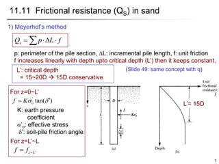
1
L’= 15D
11.11 Frictional resistance (QS) in sand
1) Meyerhof’s method
  

s
Q p L f
p: perimeter of the pile section, L: incremental pile length, f: unit friction
f increases linearly with depth upto critical depth (L’) then it keeps constant.
'
tan( )
 
 o
f K
For z=0~L’
For z=L’~L
K: earth pressure
coefficient
’o: effective stress
’: soil-pile friction angle
L’: critical depth
= 15~20D  15D conservative
'
z L
f f 

(Slide 49: same concept with q)

2
K: Effective earth coefficient
Pile type K
Bored or jetted
Low-displacement (open ended)
High-displacement (closed ended)
1 sin '
o
K K 
? -
(1~1.4) (1~1.4)(1 sin ')
o
K K 
? -
(1~1.8) (1~1.8)(1 sin ')
o
K K 
? -
’: friction angle between soil and pile
Pile material ’
Steel ’=(0.67~0.83)’
Concrete ’=(0.9~1.0)’
Timber ’=(0.8~1.0)’

3
0.93
@ / 33.3, 35o
K
L D 

 
2) Coyle and Castello’s method
Data from 24 large scale field tests
of driven piles in sand
: Average effective
overburden pressure
’=0.8’: soil-pile friction angle
K: lateral earth pressure
coefficient  f(L/D, ’)
o
( tan )
tan(0.8 ')
 
 
 
 


o
S av
o
Q f pL K pL
K pL

4
Example 11.5
• A concrete pile is 15m(L) long and 0.45mX0.45m in cross section.
The pile is fully embedded in sand for which =17kN/m³and ’=35˚.
Calculate the ultimate skin friction, Qs
– a. Meyerhof’s method: Use K=1.3 and
– B. The method of Coyle and Castello.
' '
0.8
 

15 (15)(0.45) 6.75
   
L D m
'
0 0
0
f
 

For Z=0 to L’ For Z= L’ to L
'
z L
f f 

At z = 6.75m
At z = 0m
Part a: Meyerhof’s method
1) Critical Depth
'
tan( )
 
 o
f K
L’= 15D
' 2
0
'
2
(6.75)(17) 114.75 /
tan( ) (1.3)(114.75)[tan(0.8 35)]
79.3 /
o
kN m
f K
kN m

 
 

  

D=0.45m

5
Example 11.5
0 6.75
6.75
' ( ')
2
0 79.3
(4 0.45)(6.75) (79.3)(4 0.45)(15 6.75)
2
481.75 1177.61 1659.36 1659
 


 
  
 
 

 
    
 
 
   
z z m
s z m
f f
Q pL f p L L
kN kN
L’= 15D
2) Ultimate skin friction, Qs
Part b: Coyle and Castello’s method
Part b: Coyle and Castello’s method
tan(0.8 ')
 

 o
S
Q K pL
/ 15/0.45 33.3; 35 0.93

    
L D K
(0.93)(127.5)tan[(0.8 35)](4 0.45)(15) 1702
s
Q kN
   
2
(15)(17)
127.5 /
2
  
o kN m

6
Part c: Using the results of Part d of Example 11.1,
estimate the allowable bearing capacity of the pile (Use FS=3)
Example 11.5
1250 1680
977
3
p s
all
Q Q
Q kN
FS
 
  
Average value of Qs from part a and b
From part d of Example 11.1, Qp=1250kN
( )
1659 1702
1680.5 1680
2
s average
Q kN

  

7
3) Correlation with SPT (Meyerhof)
2
60
2
60
( / ) 2( )
( / ) 0.2( )
av
av
f kN m N
f t m N
=
=
High displacement driven pile
Low displacement driven pile

s av
Q pLf
2
60
2
60
( / ) 1( )
( / ) 0.1( )
av
av
f kN m N
f t m N
=
=
: the average of SPT N-value
60
( )
N
MRT: 0.3N

8
Example 11.4
Refer to the pile describe in Example 11.3.
Concrete pile, L=15.2m, A=305mmX305mm.
Q: Estimate the magnitude of Qs for pile.
Depth below
ground
surface (m)
N60
1.5 8
3.0 10
4.5 9
6.0 12
7.5 14
9.0 18
10.5 11
12.0 17
13.5 20
15.0 28
16.5 29
18.0 32
19.5 30
21.0 27
2
60
( / ) 2( )
av
f kN m N
=
High displacement driven pile
.
N
+ + + + + + + + +
= = ?
60
8 10 9 12 14 18 11 17 20 28
14 7 15
10
(4 0.305)(15.2)(30) 556.2
s av
Q pLf kN
   
Allowable load-carrying capacity (Use FS=3)
893 556.2
483
3
p s
all
Q Q
Q kN
FS
 
  
2
60
2( ) (2)(15) 30 /
  
av
f N kN m

9
' c
f f

= '

     
  c
s
Q p L f p L f
4) Correlation with CPT
’ for electric cone penetrometer ’ for mechanical cone penetrometer
' 0.44
@ / 16
z D
 

f: unit skin friction; fc: frictional resistance (CPT)

10
Example 11.6
Concrete pile: 305mmX305mm, L=18m
Fully embedded in a sandy soil
CPT (mechanical cone results)
Q: Estimate the allowable load (Use FS=3)
Qp = Apqc = (0.305*0.305)(9500) = 883.7kN
Depth from
ground
surface (m)
qc
(kN/m2
)
fc
(kN/m2
)
0-5 3040 73
5-15 4560 102
15-25 9500 226
1) End bearing: c
p q
q  (in granular soils: Meyerhof)
1107.35
s
Q kN

883.7 1107.35 1991.05
u p s
Q Q Q kN
    
L/D
= 5/0.305
= 16
1991.05
663.68 664
3
u
all
Q
Q kN
FS
   
2) Skin friction
3) Ultimate and allowable loads
Depth from ground
surface (m)
△L
(m)
fc (kN/m2
) α' p
p△Lα'fc
(kN)
0-5 5 73 0.44 4*0.305 195.9
5-15 10 102 0.44 1.22 547.5
15-25 3 226 0.44 1.22 363.95

11
11.12 Frictional (Skin) resistance in Clay
• Clay  QP is small  QS is important
– , ,  methods
 method: total stress + effective stress
 method: total stress
 method: effective stress
– Correlation with CPT

12
• Suggested by Vijayvergiya & Focht (1972)
– Based on the assumption that the
displacement of soil casued by pile
driving results in a passive lateral
pressure at any depth
• Average unit skin resistance
 depends on the penetration depth
( 2 )
 
 
av o u
f c
1)  method: total stress + effective stress
S av
Q pLf

Average skin resistance
0.136
@ 30
L m
 


13
• Average unit skin resistance
– cu =(L1cu1+L2cu2+L3cu3+․․․)/L : mean undrained shear strength
– =(A1+A2+A3+․․․)/L : mean vertical effective stress
for the entire embedment depth
o
 ¢
( 2 )
 
 
av o u
f c

14
11.12 Frictional resistance in Clay

 
= =
檍
s u
Q fp L c p L
• Suggested by Tomlinson
• Unit skin friction

= u
f c
2)  method: total stress
.
0 45

 o
u
C
c
念 ¢÷
ç
= ÷
ç ÷
÷
ç
曜
: empirical adhesion factor
C  0.4~0.5: bored piles
C  0.5: driven piles
Soft:  = 1
Stiff:  < 1
Table 11.10

15

= å
S
Q fp L
• Suggested by Burland(1973)
• Pile driving in saturated clay  Generation of excess pore water pressure
 Dissipation  effective stress
o
f '


σ’0 = vertical effective stress
β = K tan’R
’R =drained friction angle of remolded clay
K = earth pressure coefficient
NC clay
OC clay
1
1


= -
= -
'
'
( sin )
( sin )
R
R
K
K OCR
3)  method: effective stress
OCR: overconsolidation ratio

16
• Suggested by Schmertmann (1975)
4) Correlation with CPT
f: unit skin friction
fc: frictional resistance (CPT)
' c
f f

=
'

     
  c
s
Q p L f p L f
' c
f f

=
Same equation in sand and clay
But is pretty much different
' c
f f

=
 '
'

     
  c
s
Q p L f p L f

17
Example 11.7
Top 10m: NC clay
Bottom: OC clay (OCR=2)
A driven pipe pile in clay
OD=406mm
Q: Calculate the skin resistance
By 1)  method; 2)  method; 3)  method (’R=30o)
(0.406) 1.275

 
p m
1)  method: total stress 
 
= =
檍
s u
Q fp L c p L
Depth from ground
surface (m)
△L(m) Cu(kN/m2
) Cu/Pa  αCup△L(kN)
0-5 5 30 0.3 0.82 156.83
5-10 5 30 0.3 0.82 156.83
10-30 20 100 1.0 0.48 1224.0
Qs=1538kN

18
Example 11.7
( 2 )
 
 
av o u
f c
(1) 1 (2) 2 (3) 2
2
30
(30)(5) (30)(5) (100)(20)
76.7 /
30
 

 
 
u u u
u
c L c L c L
c
kN m
1 2 3
2
'
225 552.38 4577
178.48 /
30

 

 
 
o
A A A
L
kN m
2
( 2 ) 0.136(178.48 2 76.7) 45.14 /
av o u
f c kN m
 
     
(0.406)(30)(45.14) 1727
S av
Q pLf kN

  

19
Example 11.7
3)  method: effective stress
'
'
: ( sin )
: ( sin )
R
R
NC K
OC K OCR


= -
= -
1
1
' ' '
tan
o R o
f K
  
= =
' ' '
( )
0~5m: ( sin )tan ( sin )(tan )( ) . / 2
1
0 90
1 1 30 30 13 0
2
  
av R R o
f kN m
+
= - = - =
( )
.
5~10m : ( sin )(tan )( ) . / 2
2
90 130 95
1 30 30 31 9
2
av
f kN m
+
= - =
( )
. .
10~20m : ( sin ) (tan )( ) . / 2
3
130 95 326 75
1 30 2 30 93 43
2
av
f kN m
+
= - =
( ) ( ) ( )
[ ( ) ( ) ( )]
( )( . )[( )( ) ( . )( ) ( . )( )]
1 2 3
5 5 20
0 406 13 5 31 9 5 93 43 20 2670

s av av av
Q p f f f
kN
= + +
= + + =

S
Q fp L
= å

20
Example 11.7
b. Estimate the net allowable pile capacity (FS=4).
s average
Q kN

 
( )
1538 1727
1632.5
2
. .
133 1632 5 1765 5
u p s
Q Q Q kN
= + = + =
1) End bearing
133 ( 11.2)

p
Q kN Ex
2) Skin friction
3) Ultimate capacity
.
1765 5
441
4
u
all
s
Q
Q kN
F
= = ?
4) Allowable capacity
( ) 1538
s method
Q kN
   ( ) 1727
s method
Q kN
   ( ) 2670
s method
Q kN
  

21
Example 11.8
Concrete pile: 305mmX305mm, L=20m,
Saturated clay. CPT: fc
Q: Estimate the frictional resistance Qs
Correlation with CPT

= ' c
f f
Depth (m) fc (kN/m2) fc /Pa α' △L (m) p△L α'fc (kN)
0-6 34.34 0.34 0.84 6 211.5
6-12 54.94 0.55 0.71 6 285.5
12-20 70.63 0.70 0.63 8 434.2
* p = (4)(0.305)=1.22m ' 931
c
s
Q p L f kN

  


22
11.13 Point bearing capacity of piles resting on rock
Ultimate unit point resistance
( )
u lab
q
( )
1

p u
q q N
= +
tan ( '/ )
2
45 2
 
N = +
qu: unconfined compression strength of rock
’ : drained friction angle

23
11.13 Point bearing capacity of piles resting on rock
Allowable load
5
=
( )
( )
u lab
u design
q
q
1
 +
=
( )
( )
[ ( )]
u design p
P all
q N A
Q
FS
Scale effect
Scale effect
Ap: Net Area
(not plug part)
REV: Representative Elementary Volume
permeability
strength
Lab Field

24
Example: QP on Rock
Area of H-Pile (Net Area)  Table 11.1.
: HP 310X125piles: Ap=15.9X10-3 m2
 
 
( ) 2
( )
3 2
2 3 2
'
tan (45 ) 1
5 2
76 10 / 28
tan (45 ) 1 15.9 10
5 2
182
5
u lab
p
p all
q
A
Q
FS
kN m
m
kN


 
   
 
 
   
   
 

 
 

 
 
  
 
   
 
 
 
 
 
H-pile(310X125, L=26m) is driven through a soft clay layer to rest on
sandstone. Sandstone: qu(lab) = 76MN/m², ’ = 28˚.
Q: Estimate the allowable point bearing capacity (FS=5)
5
=
( )
( )
u lab
u design
q
q
1
 +
=
( )
( )
[ ( )]
u design p
P all
q N A
Q
FS
tan ( '/ )
N 
= +
2
45 2

25
Ch 11. Pile foundations
• Contents
11.1 Introduction
11.2 Types of piles and their structural characteristics
11.4 Installation of piles
11.3 Estimating pile length
11.5 Load transfer mechanism
11.6 Equations for estimating pile capacity
– QP: 11.7~ 11.10
– QS: 11.11~11.12
– Pile bearing capacity on rock: 11.13
11.14 Pile load tests
11.15 Elastic settlement of piles
11.16 Laterally loaded piles

26
11.14 Pile Load Tests (Compression test)
Dead weight = Kentledge method

27

28

29
Tension pile

30
11.14 Pile Load Test (Compression test)
Tension pile

31
Anchor

32
Anchor

33
Test procedure
1. ML (Maintained Load): load is sustained at each level until all
settlement has either stop or does not exceed a specified amount.
• SM: Slow Maintained Load Test  0.025mm/hr
• QM : Quick Maintained Load Test  2.5-15 minutes/step
• At least twice of the design load (200%)
• At least 8 load steps (25% of design load at each step)
2. CRP (Constant Rate Penetration): load is adjusted to give constant
rate of downward movement of the pile until it reaches the failure.
* Failure: downward pile movement without increasing load,
penetration of one-tenth of the diameter of the pile at the base

34
Test results
1) Load-time
2) Load-settlement

35
Test results
2) Load-settlement
Qy: Yield load
: curvature of load – settlement
curve becomes maximum
Qu: Ultimate load
: load-settlement curve
becomes vertical
Settlement
Load
Qu: Ultimate load
Qy: Yield load

36
Disturbance due to pile driving
Variation of undrained shear
strength (cu) with time around
a pile driven into soft clay
Remolded or compacted zone around a pile driven into soft clay
30~60days

37
Time effects
Setup (or freeze): capacity increase with time after installing driven piles.
Setup occurs in saturated clays and silts due to the dissipation of excess
pore pressure at the skin friction.
Relaxation: capacity decrease with time after installing driven piles.
Relaxation occurs in dense fine sand or stiff fissured clay at the pile tip.
Variation of Qs and Qp with
time for a pile driven

38
11.14 Pile Load Test (Tension or Pullout test)
• Tension, Pullout, uplift
• ML (Maintained load) or CRU (Constant rate of uplift)
• This test method was discontinued in 2003 by ASTM

39

40
11.14 Pile Load Test (Lateral loading test)
• This test method was discontinued in 2003 by ASTM
Pair of piles
(Reaction pile)
Single pile
(Kentledge weight)

41
( ) 0.012 0.1 u
u r
r p p
Q L
D
s mm D
D A E
 
  
 
 
Settlement for ultimate load Qu
u
p p
Q L
A E
0.012 0.1
r
r
D
D
D
 
  
 
Qu (kN): ultimate load
D(mm): Diameter or width
Dr: reference diameter or width (300mm)
L(mm): pile length
Ap(mm2): cross sectional area
Ep(kN/mm2): Young’s modulus of pile
Ultimate load by Davisson’s method
   
( )
( ) 3.81 609.6
120
u
u
p p
Q L
D mm
s mm D mm
A E
   
( )
( ) 3.81 609.6
30
u
u
p p
Q L
D mm
s mm D mm
A E
1) Original
2) Simplified (Design Code)

42
Example 11.9
Figure shows the load test results of a 20m long concrete pile (406mm x
406mm) embedded in sand. (Ep = 30 x 106 kN/m2)
Q: Using Davisson’s method, determine the ultimate load Qu
1) Settlement for Qu 0.012 0.1 u
u r
r p p
Q L
D
s D
D A E
 
  
 
 
2) Dr=300mm, D=406mm, L=20,000mm
Ap=164,836mm2, Ep=30x106kN/m2
(20,000)
406
(0.012)(300) 0.1
300 (30)(164,836)
3.6 0.135 0.004
3.735 0.004
u
u
u
u
Q
s
Q
Q
 
  
 
 
  
 
3) The intersection of this line with the load-
settlement curve gives the failure load
Qu =1460kN

43
The total settlement of a pile under a vertical working load Qw
se = se(1) + se(2) + se(3)
se(1) = axial deformation of pile
se(2) = pile settlement due to load at pile tip
se(3) = pile settlement due to load along pile shaft

44
( )
( )
wp ws
e
p p
Q Q L
S
A E

+
=
1
Qwp= load carried at the pile point under
working load condition
Qws= load carried by frictional (skin)
resistance under working load condition
Ap = area of cross section of pile
L = lengh of pile
Ep= modulus of elasticity of the pile material
1) se(1) : axial deformation of pile
wp
p p
Q L
A E

45
** same method discussed in shallow foundation
D : width or diameter of pile
qwp (=Qwp/Ap) : point load per unit area at the pile point
Qwp : load carried at the pile point under working load condition
Es : modulus of elasticity of soil at or below the pile point
s : Poisson’s ratio of soil
Iwp : influence factor ≈ 0.85
wp
s
s
wp
e I
E
D
q
S )
1
( 2
)
2
( 


Soil type Driven pile Bored pile
Sand 0.02 ~ 0.04 0.09 ~ 0.18
Clay 0.02 ~ 0.03 0.03 ~ 0.06
Silt 0.03 ~ 0.05 0.09 ~ 0.12
( )
wp p
e
p
Q C
S
Dq
=
2
Vesic’s semi-empirical method Table 11.13 Typical values of CP
2) se(2) : pile settlement due to load at pile tip
qp : ultimate point load of the pile
Cp: empirical coefficient
(sec 5.10: simple method
 rigid foundation)

46
p = perimeter of the pile
L= embedded length of pile
Qws/pL : average value of f along the pile shaft
Iws= influence factor
ws
e s ws
s
Q D
S I
pL E

  
 
  
 
 
2
(3) )
(1
( )
3
ws s
e
p
Q C
S
Lq
=
.
L
Iws
D
= +
2 0 35
Vesic’s semi-empirical method
CS = empirical constant
( )
. . /
0 93 0 16
S P
C L D C
= +
3) se(3) : pile settlement due to load along pile shaft
Soil type Driven pile Bored pile
Sand 0.02 ~ 0.04 0.09 ~ 0.18
Clay 0.02 ~ 0.03 0.03 ~ 0.06
Silt 0.03 ~ 0.05 0.09 ~ 0.12
Table 11.13 Typical values of CP

47
The allowable working load on a prestressed concrete pile 21-m long that
has been driven into sand is 502kN. The pile is octagonal in shape with D =
356mm. Skin resistance carries 350kN of the allowable load, and point
bearing carries the rest.
(use Ep = 21 x 106kN/m2, Es=25x103kN/m2, s=0.35, and =0.62 )
Q: Determine the settlement of the pile
From Table 11.3a : Ap=1045cm2, p=1.168m
502 350 152
Wp
Q kN
  
(1) 2 6
[152 0.62(350)](21)
0.00353 3.53
(0.1045 )(21 10 )
e
S m mm
m

  

Example 11.10
( )
( )
wp ws
e
p p
Q Q L
S
A E

+
=
1
1) se(1) : axial deformation of pile
Octagonal pile with D=356mm
Skin friction: QWS=350kN  End bearing:

48
 
2
(2)
2
3
(1 )
152 0.356
1 0.35 (0.85) 0.0155 15.5
0.1045 25 10
WP
e s WP
s
q D
S I
E
m mm

 
  
   
  

  
ws
e s ws
s
Q D
S I
pL E
m mm

  
 
  
 
 
  
   
  

 
 
2
(3) )
2
3
(1
350 0.356
(1 0.35 )(4.69) 0.00084 0.84
(1.168)(21) 25 10
69
.
4
356
.
0
21
35
.
0
2
35
.
0
2 




D
L
IWS
4) Total settlement :
(1) (2) (3) 3.53 15.5 0.84 19.96
e e e e
s s s s mm
      
2) se(2) : pile settlement due to load at pile tip
3) se(3) : pile settlement due to load along pile shaft
Example 11.10

49
• Contents
11.17 Pile driving formulas
11.18 Pile capacity for vibration-driven piles
11.19 Negative skin friction
Group piles
11.20 Group efficiency
11.21 Ultimate capacity of group piles in saturated clay
11.22 Elastic settlement of group piles
11.23 Consolidation settlement of group piles
11.24 Piles in rock

50
11.17 Pile-driving formulas
So: Set value So
Energy conservation: E(pile impact) = W(for penetration)+W(lost)
Spp : plastic deformation of pile
Sep : elastic deformation of pile
Ses : elastic deformation of soil

51
R
u
W h
Q
S C


1) Engineering News Record (ENR) formula – Ultimate capacity
WR = weight of the ram
h = height of fall of the ram
S = penetration of the pile per hammer blow
C = 2.54mm (steam hammer) ~ 25.4mm (drop hammer)
2) Based on Hammer efficiency
E
u
EH
Q
S C
=
+
2
R R p
u
R p
EW h W n W
Q
S C W W
念 + ÷
ç ÷
= ç ÷
ç ÷
ç
+ +
曜
3) Modified ENR formula
S: set value (mm/blow)
n: coefficient of restitution (0.25 ~ 0.5)
WP: weight of pile including cap
E : hammer efficiency
HE : rated energy of the hammer

52
4) Danish formula
p
p
E
E
u
E
A
L
EH
S
EH
Q
2


E : hammer efficiency
HE : rated energy of the hammer
EP: elastic modulus of pile
S: set value (mm/blow)
L: pile length
AP: cross-sectional area of pile
5) Allowable bearing capacity: Qall = Qu/ FS

53
A precast concrete pile 0.305m x 0.305m in cross section is driven by
hammer.
- Maximum rated hammer energy = 40.67kN-m
- Hammer efficiency = 0.8 - Weight of ram = 33.36kN
- Pile length = 24.39m - Coefficient of restitution(n) = 0.4
- Weight of pile cap = 2.45kN - Ep = 20.7 x 106kN/m2
- Number of blows for last 25.4mm of penetration = 8
Q: Estimate the allowable pile capacity by the modified ENR formula (FS = 6)
2) Ultimate load (Qu) :
2 2
(0.8)(40.67 1000) 33.36 (0.4) (55.95)
2697
25.4 33.36 55.95
2.54
8
R R P
u
R P
EW h W n W
Q kN
S C W W
   
  
  
   
  
 
  
1) Weight of pile +cap 3
(0.305 0.305 24.39)(23.58 / ) 2.45
55.95
P
W kN m
kN
   

Example 11.14
2697
449.5
6
u
all
Q
Q kN
FS
  
Unit weight

54
A precast concrete pile 0.305m x 0.305m in cross section is driven by
hammer.
- Maximum rated hammer energy = 40.67kN-m
- Hammer efficiency = 0.8 - Weight of ram = 33.36kN
- Pile length = 24.39m - Coefficient of restitution(n) = 0.4
- Weight of pile cap = 2.45kN - Ep = 20.7 x 106kN/m2
- Number of blows for last 25.4mm of penetration = 8
Q: Estimate the allowable pile capacity by the Danish formula (FS = 4)
Example 11.14
2
(0.8)(40.67)
1857
25.4
0.01435
8 1000
E
u
E
p p
EH
Q
EH L
S
A E
kN


 


6
(0.8)(40.67)(24.39)
0.01435 14.35
2 2(0.305 0.305)(20.7 10 )
E
p p
EH L
m mm
A E
  
 
1857
464
4
u
all
Q
Q kN
FS
  

55
Settlement of soils is greater than that of pile.
1. After a pile is driven, a clay soil is placed over a granular soil 
consolidation
2. A granular soil is placed over a soft clay  consolidation
3. Lowering of water table  increase in effective stress  consolidation
Negative skin friction = downward drag force
L1

56
Load transfer mechanism

57
K'=Ko=1-sin’ : earth pressure coefficient
o’ = f
’ z: vertical effective stress
f
’ : effective unit weight of fill
’ =(0.5 ~ 0.7)’ : soil-pile friction angle
Hf : height of fill
0 0
0
' tan '
' tan '
f f
f
H H
n n o
H
f
Q pf dz pK dz
pK z dz
 
 
¢
= =
¢
=
窒
ò
1) Clay fill over granular soil
 Similar to -method
' tan '
n o
f K  
¢
=
2
1
' tan '
2
 
n f f
Q pK H
¢
=
Unit negative skin friction

58
Example 11.16
H = 2m. Pipe pile (D=0.305 m, ’ = 0.6 ). Clay
fill (above the water table),  = 16 kN/m3,  = 32.
Q: Determine the total drag force
(0.305) 0.958
p m

= =
' (0.6)(32) 19.2
  
2
1
(0.958)(0.47)(16)(2) tan19.2
2
5.02 kN
n
Q =
=
' 1 sin ' 1 sin32 0.47
K 
= - = - =
2
1
' tan '
2
 
n f f
Q pK H
¢
=

59
2
1 1
1
( ' tan ') ' ' tan '
2
n f f
Q pK H L pK L
   
¢
= +
Negative skin friction: 0~L1 (neutral depth)
 Direction change in skin friction
 End bearing pile: L1 = L-Hf
 Friction pile (Bowles, 1982)
 Unit negative skin friction
1
1
( ) 2
2 ' '
 
 
f f f f f f
L H L H H H
L
L
念 ⇔
- - ÷
ç ÷
= + -
ç ÷
ç ÷
ç
曜
'
' tan '
 
n o
f K
=
1 1
0 0
'( ' )tan '
  
L L
n n f f
Q pf dz pK H z dz
¢
= = +
窒
2) Granular soil fill over clay
K'=Ko=1-sin’
’ =(0.5 ~ 0.7)’
 f
¢
'

L1

60
Example 11.17
Pile: OD= 0.305m, L = 20m, ’ = 0.6clay.
Sand fill: H = 2m,  = 16.5 kN/m3
Clay: clay = 34, sat(clay) = 17.2kN/m3
Water table = top of the clay layer.
Q: Determine the downward drag force.
Depth of neutral plane
1
1
2
2 ' '
 
 
f f f f f f
L H L H H H
L
L
念 ⇔
- - ÷
ç ÷
= + -
ç ÷
ç ÷
ç
曜
)
81
.
9
2
.
17
(
)
2
)(
5
.
16
)(
2
(
)
81
.
9
2
.
17
(
)
2
)(
5
.
16
(
2
2
20
2
20
1
1















L
L
Sand

Clay
clay
sat(clay)
1 1
1
242.4
8.93 11.75
L L m
L
= - ?
m
p 958
.
0
)
305
.
0
( 

44
.
0
34
sin
1
' 

 
K
' (0.6)(34) 20.4
 = =
(0.958)(0.44)(16.5)(2)[tan(20.4)](11.75)
(0.958)(0.44)(17.2 9.81)(11.75) [tan(20.4)]
2
60.78 79.97 140.75kN
n
Q
2
=
-
+
= + =
L1
2
1 1
1
( ' tan ') ' ' tan '
2
n f f
Q pK H L pK L
   
¢
= +

61
• Contents
11.17 Pile driving formulas
11.18 Pile capacity for vibration-driven piles
Group piles
11.24 Piles in rock

62
Pile spacing Pile action
< (3 ~ 7)D Group
> 7D Individual
Group pile or single pile ?

64
• Group piles
1) Bearing capacity of group piles is
extremely complicated and has
not yet been fully understood
2) Different group action of friction
piles and end-bearing piles
3) Effects of pile cap
Group effect is
greater when cap
is on the ground
Capacity
decreases
Capacity
shouldn’t be
decreased

65
( )
g u
u
Q
Q
 

Efficiency of load-bearing capacity of a group pile
 = group efficiency
Qg(u) = ultimate load-bearing capacity of
the group pile
Qu = ultimate load-bearing capacity of
each pile without the group effect

66
(1) Frictional capacity
when acting as a block
Group efficiency
pg=2(n1+n2 - 2)+4D: perimeter of block
(2) Frictional capacity
when acting individually
p: perimeter of each pile
<1.0: Qg(u) = ηΣQu
>1.0: Qg(u) = ΣQu
Capacity
1) Group efficiency of friction piles
u av
Q f pL
=
[ ]
( ) ( )
( )
g u av g av g g
av
Q f p L f L B L
f n n d D L
1 2
2
2 2 4
殞
? +
薏
= + - +

67
Name Equation
Converse-Labarre
equation
Los Angeles Group
Action equation
Seiler-Keeney
equation
2) Other equations for group efficiency of friction piles

68
3) Group efficiency of friction piles – empirical method
Ultimate capacity is reduced by 1/16 by each adjacent diagonal or row pile
Pile
type
Pile
No.
No of
adjacent pile
Reduction
factor
Ultimate capacity
A 1 8 1-8/16 1×Qu×(1-8/16) = 0.5Qu
B 4 5 1-5/16 4×Qu×(1-5/16) = 2.75Qu
C 4 3 1-3/16 4×Qu×(1-3/16) = 3.25Qu
Qg(u) = (0.5+2.75+3.25)Qu = 6.5Qu
Group efficiency
6.5
72%
9
  

69
4) Bearing capacity of group piles in Sands
Pile spacing:
CTC (center-to-center) > 3D
(1) End bearing of group pile
Qg(p) = nQp
n: pile no.
Qp: ultimate end bearing of
each pile
(2) Skin friction of group pile
Qg(s) ≥ ΣQs
due to compaction & lateral
compression (for loose sand)
(3) General: ≥1.0

70
5) Bearing capacity evaluation of group piles in sands
1) CTC > 3D
Qg(u) = ΣQu= Σ(Qp + Qs)
2) Weak layer in pile tip
smaller value from (1) and (2)
(1) Summation of individual piles
Qg(u)1=nΣQu=nΣ(Qp + Qs)
(2) Capacity of block failure
Qg(u)2 = Qg(s) + Qg(p)
Qg(s) = 2(Bg+Lg)fav(g)L
Qg(p) = End bearing of weak layer
(Bg×Lg)
3) Bored pile groups with d (CTC)≒3D
Qg(u) = (⅔～¾)ΣQu
= (⅔～¾)Σ(Qp + Qs)

71
The lower value from (1) and (2) is is Qg(u)
 
 
( ) 1 2
1 2 ( )
9
g u u P S
p u p u
Q Q n n Q Q
n n A c c p L

  
  


(1) Summation of individual pile
(2) Capacity of block failure
( ) ( ) ( )
( ) 2( )

 
   

g u g P g S
g g u p c g g u
Q Q Q
L B c N L B c L

72
34 Group pile
Square pile: 356  356mm
Center-to-center spacing: 889mm
Saturated clay
Ground water table: ground surface
Q: Allowable load-bearing capacity
of the pile group (FS=4)
Upper layer: (1) 1
/ 50.3/100 0.503 0.68

   
u a
c P
Example 11.18
(1) Summation of individual pile
 
 
( ) 1 2 ( )
1 2 ( ) 1 (1) 1 2 (2) 2
9
9
g u p u p u
p u p u u
Q n n A c c p L
n n A c c pL c pL

 
  
  

Lower layer: (2) 2
/ 85.1/100 0.851 0.51

   
u a
c P
2
9(0.356) (85.1) (0.68)(50.3)(4 0.356)(4.57)
(3)(4)
(0.51)(85.1)(4 0.356)(13.72)
14,011
u
Q
kN
 
 
  
 
 


73
(3)(0.889) 0.356 3.023
(2)(0.889) 0.356 2.134
  
  
g
g
L m
B m
Example 11.18
(2) Block failure
( ) ( ) 2( )

   

g u g g u p c g g u
Q L B c N L B c L
3.023 18.29
1.42, 8.57 8.75
2.134 2.134

     
g
c
g g
L L
N
B B
14,011 14,011
3,503
4
  
all
Q kN
FS
 
( ) ( ) 2( )
(3.023)(2.134)(85.1)(8.75) (2)(3.023 2.134) (50.3)(4.57) (85.1)(13.72)
19,217

   
   


g u g g u p c g g u
Q L B c N L B c L
kN
(3) Lower value 14,011

u
Q kN
(4) Allowable load-bearing capacity

74
Settlement of group piles (sg) is greater than settlement of single pile (s)
at equal load per pile
Sg increases with the width of group
pile (Bg) and CTC spacing of piles (d)
(Meyerhof, 1961), D: pile diameter

75
( )
g
g e e
B
S S
D
=
1) Vesic (1977)
q=Qg/(LgBg) in kN/m2
Lg & Bg = length and width of pile group section (m)
N60 =average corrected SPT N-value
within seat of settlement ( Bg deep below pile tip)
I=influence factor = 1-L/(8Bg) ≥ 0.5
L= length of embedment of piles (m)
Sg(e) = elastic settlement of group piles
Bg = width of group pile section
D = width or diameter of each pile in the group
Se= elastic settlement of each pile
at comparable working load
2) Meyerhof(1976)
( )
60
0.96
( )
g
g e
q B I
S mm
N
=

76
3) CPT correlation
( )
2
g
g e
c
qB I
S
q
=
q=Qg/(LgBg) in kN/m2
Lg & Bg = length and width of pile group section (m)
I=influence factor = 1-L/(8Bg) ≥ 0.5
L= length of embedment of piles (m)
qc = average cone penetration resistance
within the seat of settlement

77
(3 1) 2 (2)(3 ) 7 (7)(0.356 ) 2.492
2
g
D
B d D D D m m
 
       
 
 
( )
2.492
(19.69) 52.09
0.356
e g
S mm
 
34 Group pile
Octagonal pile: D=356mm Pile length L=21m
Center-to-center spacing: 3D Sandy soils
Details of each pile and the sand are described in Example 11.10
Working load of group pile = 6024kN:  34Qall = 6024kN  Qall = 502kN
Q: Estimate the elastic settlement of the pile group by Vesic method
19.96
e
s mm

1) Settlement of single pile (Example 11.10)
( )
g
g e e
B
S S
D
=
2) Vesic method
Example 11.19

78
oi
 ¢
1) Total load
Qg = Load from superstructure – effective weight of soil removed
2) Assume that Qg is transmitted at (2/3)L from top.
Load spreading  2:1 (2V:1H)
3) Effective stress increase at the middle of clay layer
Qg
( )( )
g
i
g i g i
Q
B z L z

 ¢=
+ +
i

 ¢
( )( )
g
i
g i g i
Q
B z L z

 ¢=
+ +
z
2/3L
2/3L
L

79
4) Disregard the settlement above (2/3)L
5) Settlement below (2/3)L
log
1
i oi i
ci ci
i oi oi
H
S C
e
 



念 ⇔
+ ÷
ç ÷
= ç ÷
ç ÷
ç ¢
+ 曜
å
log log
1
pi
i oi i
ci si ci
i oi oi pi
H
S C C
e
  
 


念 ¢ ⇔
+ ÷
ç ÷
ç
= + ÷
ç ÷
⇔ ÷
ç
+ 曜
å
NC clay
OC clay
6) Total settlement g ci
S S
 
= å

80
A group pile in NC clay
Q: Determine the consolidation
settlement of the piles
L=15m
2:1 distribution starts at 10m
Qg = 2000kN
(1) 1 0(1) (1)
(1)
0(1) 0(1)
' '
log
1 '
c
c
C H
S
e
 



殞殞 +
油油
= 油油
+
油油
薏薏
2
)
1
(
0 /
8
.
134
)
81
.
9
0
.
18
(
5
.
12
)
2
.
16
(
2
' m
kN





Example 11.20
Clay layer 1
2
(1)
1 1
2000
' 51.6 /
( )( ) (3.3 3.5)(2.2 3.5)
g
g g
Q
kN m
L z B z

 = = =
+ + + +
(1)
(0.3)(7) 134.8 51.6
log 0.1624 162.4mm
1 0.82 134.8
c
S m

殞 +
油
= = =
油
+ 薏
Clay1
Clay2
Clay3

81
(2) 2 0(2) (2)
(2)
0(2) 0(2)
' '
log
1 '
c
c
C H
S
e
 



殞殞 +
油油
= 油油
+
油油
薏薏
2
)
2
( /
52
.
14
)
9
2
.
2
)(
9
3
.
3
(
2000
' m
kN





(2)
(0.2)(4) 181.62 14.52
log 0.0157 15.7mm
1 0.7 181.62
c
S m

殞 +
油
= = =
油
+ 薏
Clay layer 2
2
(2)
' 2(16.2) 16(18.0 9.81) 2(18.9 9.81) 181.62 /
o kN m
 = + - + - =
2
(3)
2000
' 9.2 /
(3.3 12)(2.2 12)
kN m

 = =
+ +
( ) 162.4 15.7 5.4 183.5mm
c g
S
 = + + =
Clay layer 3
(3)
(0.25)(2) 208.99 9.2
log 0.0054 5.4mm
1 0.75 208.99
S m

殞 +
油
= = =
油
+ 薏
2
0(3)
' 181.62 2(18.9 9.81) 1(19 9.81) 208.99 /
kN m
 = + - + - =
Total settlement
Example 11.20
(3) 0(3) (3)
(3)
0(3) 0(3)
3 ' '
log
1 '
c
c
C H
S
e
 



殞殞 +
油油
= 油油
+
油油
薏薏

82
11.24 Bearing capacity of group piles in rock
Point bearing group piles
( ) 300
g u u
Q Q if d D mm
  


83
• Assignment # 11-1 (Capacity)
– Due: Next Week
– Problems: 11.1 ~ 11.5 // 11.10, 11.11
• Assignment # 11-2 (Settlement)
– Due: (Saturday)
– Problems: 11.13 // 11.16~11.18 // 11.20, 11.21
• Assignment # 11-3 (Group pile)
– Due: (Saturday)
– Problems: 11.23, 11.25 // 11.26
Homework Assignment - Chapter 11

84
3rd Exam
December 10 (Saturday) 10:00 ~ 13:00
Chapter 6 & 11
Closed book
Calculator
No Smart Devices
Announcement

85
Weight Remarks
Attendance &
Participation
15%
The student should attend more than 3/4 of the
classes scheduled.
Personal meeting.
Homework
Assignments
20%
Homework will be given weekly (or biweekly
depending on the topics).
It should be handed in a week after the date assigned.
Examinations 70%
1st Option: 70/3=23.3% each
2nd Option: 15%, 20%, 35%
 Grade is based on the better one.
Grading

86
Setup
ASTM D 4945
Pile Driving Analyzer (PDA)

87
Wave propagation in pile (1D)
• Smith Model (1960)
– Pile : lumped mass
spring
– Soil : viscoelastic-plastic
• 1D wave Equation
R
x
u
E
t
u






2
2
2
2


88
Proportionality
• Wave speed
• Strain
• Particle Velocity
• Rearrangement
• EA 













E
t
L
c
c
t
L 







t
V



ZV
V
c
EA
F 

c
V



89
• Piles driven to rock
– Notes
– H형 강말뚝, 강관말뚝, 콘크리트 말뚝과 암반간의 정확한 접촉면적 산정 어려움
– 지지력은 암석의 종류와 특성, 말뚝의 암석내 근입깊이 등에 좌우
– 지지력에 대한 해석적 접근이 어려움
– 재하시험에 의한 확인이 정확
– 재하시험등에 의해 누적된 경험적 데이터나 항타시 관입량으로 지지력 추정
– 말뚝선단의 손상 가능성
• 극한선단지지력 (Goodman, 1980)
• 여기서,
• qu = 암석의 일축압축강도, qu(design) = qu(lab)/
Piles driven to rock
암석종류 내부마찰각, Φ
sandstone 27～45
limestone 30～40
shale 10～20
granite 40～50
marble 25～30

90
11.2 Types of piles and Their Structural Characteristics
• Concrete piles
• Allowable structure capacity
– AC : cross-sectional area of the concrete
– fC : allowable stress of concrete (0.25f’)
all C C
Q A f

Advantage Disadvantage
Easy to handle: cutoff, extension
High driving resistance (0.9fy)
High loading capacity
Relatively costly
Noise during driving
Corrosion

91
• 1. Class A piles carry heavy loads. The minimum diameter
of the butt should be 356mm(14in).
• 2. Class B piles are used to carry medium loads. The
minimum butt diameter should be 305~330mm(12~13in).
• 3. Class C piles are used in temporary construction work.
They can be used permanently for structures when the
entire pile is below the water table. The minimum butt
diameter should be 305mm(12in).
Timber piles

92
11.3 Estimating pile length
• Load transfer mechanism
A. point bearing piles
B. friction piles
C. compaction piles

93
11.3 Estimating pile Length
• Selecting the piles
– C. compaction piles
• Under certain circumstances, piles are driven in granular soils
to achieve proper compaction of soil close to the ground surface.
These piles are called compaction piles.
• The lengths of compaction piles depend on factors such as (a)
the relative density of the soil before compaction, (b) the desired
relative density of the soil after compaction, and (c) the required
depth of compaction.

94
11.11 Other correlations for calculating QP with CPT and SPT
• LCPC
– According to the LCPC method,
• where qc(eq) = equivalent average cone resistance
kb = empirical bearing capacity factor
b
eq
c
p k
q
q )
(


95
• LCPC
The magnitude of qc(eq) is calculated in the following
manner :
– 1. Consider the cone tip resistance qc within a range of 1.5D below
the pile tip to 1.5D above the pile tip, as shown in Figure 11.15.
– 2. Calculate the average value of qc[qc(av)] within the zone shown in
figure 11.15.
– 3. Eliminate the qc values that are higher than 1.3qc(av) and the qc
values that are lower than 0.7qc(av).
– 4. Calculate qc(eq) by averaging the remaining qc values.
– Briaud and Miran (1991) suggested that
• Kb = 0.6 (for clay and silts)
• Kb = 0.375 (for sands and gravels)

97
• Dutch
– 1. Average the qc values over a distance yD below the pile tip. This
is path a-b-c. Sum qc values along the downward path a-b (i.e., the
actual path) and the upward path b-c (i.e., the minimum path).
Determine the minimum value qc1 = average value of qc for
0.7< y< 4.
– 2. Average the qc values (qc2) between the pile tip and 8D above
the pile tip along the path c-d-e-f-g, using the minimum path and
ignoring minor peak depressions.
– 3. Calculate
a
b
c
c
p p
k
q
q
q 150
'
2
)
( 2
1




98
• Figure 11.16
Dutch
method

99
• Dutch
– DeRuiter and Beringen(1979) recommended the following
values for k’b for sand :
• 1.0 for OCR = 1
• 0.67 for OCR = 2 to 4
– Nottingham and schmertmann (1975) and schmertmann
(1978) recommended the following relationship for qp in clay:
a
b
c
c
p p
k
q
q
R
R
q 150
'
2
)
( 2
1
2
1 



100
• α 방법 (Tomlinson, 1971)
– Total stress parameters of the clay for short term load capacity
– 여기서,cu=점토의 비배수 전단강도,
– α=adhesion factor
– API (1974) for N.C. clay and short piles
– For very long piles, α=αpF
• 상재하중 증가로 인한 비배수 전단강도의 증가효과를 normalization
• 항타시 진동 및 bending으로 인한 주면마찰의 감소 고려

101
Solve Example 11.8 by Broms’s method. Assume that pile is flexible and
is free headed. Let the yield stress of pile material, Fy=248MN/m2; the
unit weight of soil, =18kN/m3; and the soil friction angle =35.
Solution
We check for bending failure. From Eq. (11.100),
From Table 11.1a,
Also,
and
y
y SF
M 
2
254
.
0
10
123
2
6
1




d
I
S
p
kNm
M y 2
.
240
)
10
248
(
2
254
.
0
10
123 3
6















8
.
868
2
35
45
tan
)
18
(
)
254
.
0
(
2
.
240
2
'
45
tan 2
4
2
4
4




















D
M
K
D
M y
p
y
Example 11.9

102
From Figure 11.37a, for My/D4Kp=868.8, the magnitude of Qu(g)/KpD3  (for a
free-headed pile with e/D=0) is about 140, so
Next, we check for pile head deflection. From Eq. (11.101),
so
From Figure 11.38a, for L=21.5, e/L=0 (free-headed pile): thus,
kN
D
K
Q p
g
u 4
.
152
)
18
(
)
254
.
0
(
2
35
45
tan
140
140 3
2
3
)
( 








 
1
5
6
6
5 86
.
0
)
10
123
)(
10
207
(
000
,
12 





 m
I
E
n
p
p
h

5
.
21
)
25
)(
86
.
0
( 

L

ion)
interpolat
(by
15
.
0
)
(
)
( 5
/
2
5
/
3

L
Q
n
I
E
x
g
h
p
p
o

103
and
Hence, Qg=40.2kN(<152.4kN).
kN
L
n
I
E
x
Q
h
p
p
o
g
2
.
40
)
25
)(
15
.
0
(
)
000
,
12
(
)]
10
123
)(
10
207
)[(
008
.
0
(
15
.
0
)
(
)
(
5
/
2
5
/
3
6
6
5
/
2
5
/
3







104
Consider a 20-m-long steel pile driven by a Bodine Resonant Driver (Section
HP 310  125) in a medium dense sand. If Hp = 350 horsepower, p = 0.0016
m/s, and  = 115 Hz, calculate the ultimate pile capacity, Qu.
Solution
From Eq. (11.122),
For an HP pile in medium dense sand, SL  0.762  10-3m/cycle. So
f
S
H
Q
L
p
p
p
u





98
746
.
0
kN
2928




 
)
115
)(
10
762
.
0
(
0016
.
0
)
0016
.
0
)(
98
(
)
350
(
746
.
0
3
u
Q
Example 11.11

105
11.8 Janbu’s method for estimating QP
* *
' '
p p c q
Q A c N q N
 
 
 
* 2 2
(tan ' 1 tan ') exp(2 'tan ')
q
N    
  
* *
( 1)cot '
c q
N N 
 
:
'

:
'


 p
p
p N
q
A
Q '
20
54
,
35 


 

q
q N
N 



kN
1033
)
45
.
0
45
.
0
(
20
)
17
15
( 






106
1) For Φ’=30˚  Nq*≈55 (Figure 11.22)
Example 11.1 (old)
• A concrete pile is 16m(L) long and 410mmX410mm in cross section. The
pile is fully embedded in sand for which γ=17kN/m³and Φ’=30˚.
Calculate the ultimate point load, Qp, by
– a. Meyerhof’s method (section 11.7).
– b. Vesic’s method (section 11.8), Use Ir = Irr = 50.
– c. Janbu’s method (section 11.9), Use η’=90˚.
kN
m
Qp 2515
)
55
)(
17
16
)(
41
.
0
41
.
0
( 2




[ ]
0 5
0 41 0 41 0 5 100 55 30 267

=
= ?
*
( . tan ')
( . . ) ( . )( )( )tan
p
p a q
Q A p N
kN
* *
' ( )

  
p p q p q p l
Q A q N A L N A q
*
0.5 tan '


l a q
q p N
2) Limiting point resistance 267
=
p
Q kN

107
Example 11.1 (old)
For Φ’=30˚ and η’=90˚ Np*= 18.4(Table 11.5)
1 2 1 30
0 41 0 41 0 16 17 36 1097
3
殞 + -
油
= ? ?
油
薏
( sin )
( . . ) ( )( )( )
P
Q kN
0 41 0 41 16 17 18 4 841
= 눼 =
( . . )( )( . )
p
Q kN
Part b: Vesic’s Method
' 1 2
( ) '
3
o
o
K
q

+
=
'
* *
( ' )
o
p p p p c
Q A q A c N N

   Ko = 1-sin()
For Φ’=30˚, Irr = 50  Nσ* =36 (Table 11.4)
Part c: Janbu’s Method
* *
' '
p p c q
Q A c N q N
 
 
 
* 2 2
(tan ' 1 tan ') exp(2 'tan ')
q
N    
  

108
Part a
Eq (11.14):
1) L’≈15D=15(0.41m)=6.15m
2) z=0, σ’o =0, f=0
z=L’=6.15m, σ’o =γL’=(17)(6.15)=104.55kN/m²
f=Kσ’otan=(1.3)(104.55)[tan(0.8x30)]=60.51kN/m²
Example 11.2 (old)
• For the pile described in Example 11.1: Concrete pile, L=16m,
A=410mmX410mm. Sand: γ=17kN/m³and Φ’=30˚.
a. Given that K=1.3 and =0.8Φ’. Determine the frictional resistance Qp,
Use Eqs. (11.14),(11.38), and (11.39)  Meyerhof’s method.
b. Using the results of Example 11.1 and Part a of this problem, estimate
the allowable load-carrying capacity of the pile. Let FS=4.
0 6 15
6 15
2
0 60 51
4 0 41 6 15 60 51 4 0 41 16 6 15 305 2 977 5 1282 7
2
= =
+
= + -
+
= ? ? = + =
.
.
( ) ' ( ')
.
( )( . )( . ) ( . )( . )( . ) . . .
z z m
s m
f f
Q pL f p L L
kN
 
 f
L
p
Qs
'
tan( )
o o
f K  

'

 z L
f f
For z=0~L’
For z=L’~L

109
Example 11.2 (old)
Part b
1
735 1282 7 504 4
4
= = + =
( . ) .
u
all
Q
Q kN
FS
s
p
u Q
Q
Q 

=
u
all
Q
Q
FS
Ultimate load
Allowable load
267 1097 841
735
3
+ +
= ?
P
Q kN 1282 7
= .
S
Q kN

110
Example 11.3
• Consider a concrete pile in sand. Concrete pile, L=15.2m,
0.305mX0.305m. Variations of N60 with depth are shown in this table .
Q: Estimate Qp – a. Using Meyerhof’s method
b. Using Briaud’s method
Depth below ground suface(m) N60
1.5 8
3.0 10
4.5 9
6.0 12
7.5 14
9.0 18
10.5 11
12.0 17
13.5 20
15.0 28
16.5 29
18.0 32
19.5 30
21.0 27
24
5
.
23
4
29
28
20
17
60 





N
60
60 4
4
.
0 N
p
D
L
N
p
q a
a
p 

Eq.(11.37) :
1) N60 of 5D ~ 10D (D:0.305m)
2) From eq.(11.37)
60
60 4
]
4
.
0
[
)
(
N
p
A
D
L
N
p
A
q
A
Q
a
p
a
p
p
p
p




111
Example 11.3
kN
N
p
A
kN
D
L
N
p
A
a
p
a
p
893
)]
24
)(
100
)(
4
)[(
305
.
0
305
.
0
(
)
4
.
0
(
6
.
4450
)]
305
.
0
2
.
15
)(
24
)(
100
)(
4
.
0
)[(
305
.
0
305
.
0
(
]
4
.
0
[
60
60






2) From eq.(11.37)
Thus Qp=893kN
Part a: Briaud’s method
1) From Eq.(11.37)
kN
N
p
A
q
A
Q a
p
p
p
p
4
.
575
]
)
24
)(
100
)(
7
.
19
)[(
305
.
0
305
.
0
(
]
)
(
7
.
19
[
36
.
0
36
.
0
60






112
Example 11.4
Refer to the pile describe in Example 11.3. Concrete pile, L=15.2m,
A=305mmX305mm.
Q: Estimate the magnitude of Qs for pile.

113
Part a: Use Eq. (11.45).
Example 11.4
60
0.02 ( )
av a
f P N

.
N
+ + + + + + + + +
= = ?
60
8 10 9 12 14 18 11 17 20 28
14 7 15
10
2
60
0.02 ( ) (0.02)(100)(15) 30 /
av a
f P N kN m
  
(4 0.305)(15.2)(30) 556.2
s av
Q pLf kN
   
Part b: Use Eq. (11.47).
0.29 0.29 2
60
0.224 ( ) (0.224)(100)(15) 49.13 /
av a
f P N kN m
  
0.29
60
0.224 ( )
av a
f P N

(4 0.305)(15.2)(49.13) 911.1
s av
Q pLf kN
   

114
Part c: Considering the results in Example 11.3, determine the allowable
load-carrying capacity of the pile based on Meyerhof’s method and
Briaud’s method. (Use FS=3)
Example 11.4
893 556.2
483
3
p s
all
Q Q
Q kN
FS
 
  
Meyerhof’s method:
Briaud’s method :
575.4 911.1
495.5
3
p s
all
Q Q
Q kN
FS
 
  
So the allowable pile capacity may be taken to be about 490kN

115
Example 11.3 (OLD)
• For the pile described in Example 11.1Concrete pile, L=16m,
A=410mmX410mm. Sand: γ=17kN/m³and Φ’=30˚.
Q: Estimate Qall using Coyle and Castello’s method. (FS=4)
17 16 25 0 41 0 41
17 16
0 2 0 8 30 4 0 41 16
2
1143 317 8 1460 8
= 눼
´
+ 눼
= + =
( )( )( . . )
( . )( )tan( . )( . )( )
. .
u
Q
kN
s
p
u Q
Q
Q 

Ultimate load *
'

p q p
Q q N A ' tan(0.8 )
 
 o
S
Q K pL
1460 8
365 2
4
= = =
.
.
u
all
Q
Q kN
FS
For Φ’=30˚, L/D=39  Nq*=25, K≈0.2

116
11.14 General comments and allowable pile capacity
Net ultimate end bearing load
= -
( ) ( ) '
p net p gross p
Q Q q A
For soils ’>0 =
( ) ( )
p net p gross
Q Q
For soils ’=0, Nq*=1  
*
( ) ' '
 
p gross c p
Q c N q A
 
* *
( ) ' ' ' ' 9
 
     
 
p net p p u p p
c c
Q c N q q A c N A c A Q

117
Example 11.4 (Old)
( . ) .
p
A D m
 
= = =
2 2 2
0 406 0 1295
4 4
A driven pipe pile in clay. OD=406mm, t=6.35mm.
a. Calculate the net point bearing capacity. Eq.(11.19).
9

p u p
Q c A
9 9(100)(0.1295) 116.55
  
p u p
Q c A kN

118
0
30
60
90
120
150
180
200
210
230
240
243
245
248
176
100
50
0
0
5
10
15
20
25
30
35
40
45
50
0 20 40 60 80 100 120 140 160 180 200 220 240 260 280 300
침하량)mm)
하중(ton)

119
Example 11.7 (old)
PC Pile (L=12m, 305*305mm, Ep=21X106kN/m²) is driven into a homogeneous
layer of sand: d= 16.8kN/m³, Φ’= 35˚, Qall=338kN, Es=30,000kN/m², and μs=0.3.
QP=240kN, QS=98kN. Q: Determine the elastic settlement of the pile.
se = se(1) + s e(2) + se(3) = 1.48+8.2+0.64=10.32mm
( )
( ) [ ( . )( )]
. .
( . ) ( )
wp ws
e
p p
Q Q L
S m mm
A E

+ +
= = = =
´
1
2 6
97 0 6 240 12
0 00148 1 48
0 305 21 10
( )
( . )( . )
( ) [ ]( . )( . ) . .
wp
e s wp
s
q D
S I m mm
E

= - = - = =
2 2
2
1042 7 0 305
1 1 0 3 0 85 0 0082 8 2
30000
Iwp =influence factor ≈ 0.85
ws
s
s
wp
e I
E
D
pL
Q
S )
)
3
(
2
1
(
)
( 

 2
.
4
305
.
0
12
35
.
0
2
35
.
0
2 




D
L
Iws
mm
m
Se 64
.
0
00064
.
0
)
2
.
4
)(
3
.
0
1
)(
30000
305
.
0
(
)
12
)(
305
.
0
4
(
240 2
)
3
( 




se = se(1) + s e(2) + se(3)
2012 기말

120
A precast concrete pile 24.4m long that has been driven by hammer. The pile is
octagonal in shape with D = 254mm.
Q: Determine the ultimate load (by Modified ENR method)
1) Area (Table 11.3a):
4 2
645 10
p
A m

 
2) Weight of pile itself :
kN
m
kN
m
L
A
W c
p
pi 1
.
37
)
/
58
.
23
)(
4
.
24
)(
10
645
( 3
4



 

3) Cap weight : 2.98
Cap
W kN

4) Pile weight : kN
Wp 08
.
40
98
.
2
1
.
37 


5) Hammer : (1) Rated energy = 26.03kN-m = HE = WRh
(2) Ram weight : WR = 22.24kN
(3) Hammer efficiency : E = 0.85
6) Coefficient of restitution : n = 0.35
11.20 Pile-driving formulas (Example)

121
7) Ultimate load (Qu) with set value (S=2.54mm)
2
29.43 /
u
u
p
Q
q MN m
A
 
11.20 Pile-driving formulas (Example)
. ( . ) . . ( . )
. . . .
2
2
0 85 26 03 1000 22 24 0 35 40 08
1898
2 54 2 54 22 24 40 08
R R p
u
R p
EW h W n W
Q
S C W W
kN
念 + ÷
ç ÷
= ç ÷
ç ÷
ç
+ +
曜
念
? ÷
ç ÷
= =
ç ÷
ç ÷
ç
+ +
曜
8) Unit ultimate load (qu)

122
Example 11.10 (old)
A precast concrete pile 12 in12in. in cross section is driven by a hammer. The
maximum rated hammer energy E= 26 kip-ft, the weight of the ram WR= 8 kip, the
total length of the pile L= 65 ft, the hammer efficiency E = 0.8, the coefficient of
restitution n= 0.45, the weight of the pile cap Wc= 0.72 kip, and the number of
blows for the last 1 in. of penetration = 5  S=1/5 = 0.2 (in/blows).
It looks like a drop hammer  C=0.1
Q: Estimate the allowable pile capacity by using
a. the EN formula with FS = 6.
( . )( )( / )
kip
. . ( )
E
u
EH Kip ft in ft
Q
S C in
-
= = =
+ +
0 8 26 12
832
0 2 0 1
138.7 kip
u
all
Q
Q
FS
= = =
832
6

123
Example 11.10 (old)
A precast concrete pile: 12 in12in L= 65 ft. Hammer - E= 26 kip-ft, WR= 8 kip, E =
0.8, n= 0.45, Wc= 0.72 kip, S=1/5 = 0.2 (in/blows). C=0.1
b. the modified EN formula with FS = 4.
R R p
u
R p
EW h W n W
Q
S C W W
+
=
+ +
2
3
Weight of piles (65 ft)(1 ft 1 ft)(150 lb/ft ) lb 9.75 kip
p c
WA 
= = ? =
9750
weight of pile weight of cap = 9.75 0.72 10.47 kip
p
W = + + =
( . )( )( ) ( . ) ( . )
( )( . ) . kip
. . .
u
Q
殞
殞 +
油
油
= = =
油
油 + +
薏薏
2
0 8 26 12 8 0 45 10 47
832 0 548 455 39
0 2 0 1 8 10 47
.
114 kip
u
all
Q
Q
FS
= = =
455 9
4

124
Example 11.10 (old)
A precast concrete pile: 12 in12in L= 65 ft. Hammer - E= 26 kip-ft, WR= 8 kip, E =
0.8, n= 0.45, Wc= 0.72 kip, S=1/5 = 0.2 (in/blows). C=0.1
c. the Danish formula with FS = 3.
p
p
E
E
u
E
A
L
EH
S
EH
Q
2


( . )( )( )
0.475 in
( )( )
E
p p
EH L
A E
눼
= =
念´ ÷
ç ÷
´ ç ÷
ç ÷
ç
曜
6
0 8 26 12 65 12
2 3 10
2 12 12
1000
kip
8
.
369
475
.
0
2
.
0
)
12
)(
26
)(
8
.
0
(



u
Q
369.8
123.3 kip
3
u
all
Q
Q
FS
= = =
Concrete pile: Ep = 3106 lb/in2

125
n1 = 4, n2 = 3, D = 305mm (square pile), d = 1220mm, L =
15m. Soil: homogeneous saturated clay. cu = 70kN/m2, 
= 18.8kN/m3, Groundwater table is located at a depth
18m below the ground surface. Q: determine the
allowable load-bearing capacity of the group pile (FS=4).
Example 11.14 (old)  2012년 기말
1. Summation of individual pile
( )1 1 2 ( )
[9 ]
g u n p u p u
Q Q n n A c pc L
 
= = +
檍
2
093
.
0
)
305
.
0
)(
305
.
0
( m
Ap 

m
p 22
.
1
)
305
.
0
)(
4
( 

496
.
0
141
70
'0



u
c
2
0 /
141
)
8
.
18
(
2
15
' m
kN









kN
Qn
463
,
11
)
7
.
896
59
.
58
(
12
)]
15
)(
70
)(
22
.
1
)(
7
.
0
(
)
70
)(
093
.
0
)(
9
)[(
3
)(
4
(






average value of the effective overburden pressure
Figure 11.24 =0.7

126
n1 = 4, n2 = 3, D = 305mm (square pile), d = 1220mm, L = 15m. Soil: homogeneous
saturated clay. cu = 70kN/m2,  = 18.8kN/m3, Groundwater table is located at a depth
18m below the ground surface. Q: determine the allowable load-bearing capacity of the
group pile (FS=4).
2. Block failure
*
( )2 ( ) 2( )
g u g g u p c g g u
Q L B c N L B c L

= + +
å
( )
1
( 1) 2 / 2 (4 1)(1.22) 0.305 3.965
g
L n d D m
= - + = - + =
( )
2
( 1) 2 / 2 (3 1)(1.22) 0.305 2.745
g
B n d D m
= - + = - + =
46
.
5
745
.
2
15


g
B
L
44
.
1
745
.
2
965
.
3


g
g
B
L
.
6
.
8
*

c
N
( )2 (3.965)(2.745)(70)(8.6) 2(3.965 2.745)(70)(15)
6552 14,091 20,643
g u
Q
kN
= + +
= + =
3. Allowable capacity kN
kN
Q u
g 643
,
20
463
,
11
)
( 

( )
( )
11,463
2,866kN
4
g u
g all
Q
Q
FS
= = ?
Example 11.14 (old)

127
Anchor

기초공학 - 11-2 Pile Foundations.pdf

More Related Content

What's hot

Similar to 기초공학 - 11-2 Pile Foundations.pdf

Recently uploaded

기초공학 - 11-2 Pile Foundations.pdf