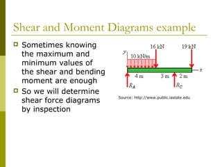
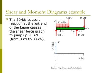
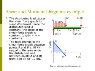
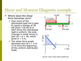
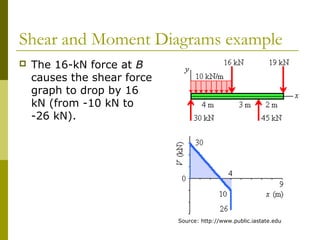
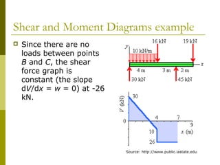
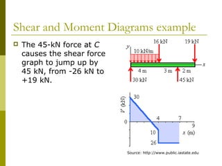
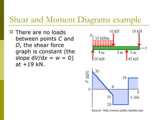
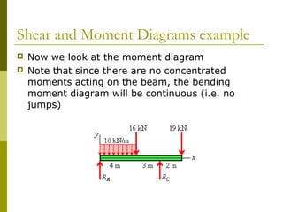
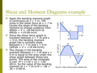
This document reviews beam theory and provides an example of calculating shear force and bending moment diagrams for a beam with various loads applied. The example beam is loaded with a uniform distributed load, two concentrated loads, and supported with two reactions. Free body diagrams are drawn and the reactions are calculated. Then, the shear force and bending moment are calculated as functions of position along the beam based on the loads and reactions. Shear and bending moment diagrams are drawn to visualize how the values change along the length of the beam.

1. Eng. 6002 Ship Structures 1
Hull Girder Response Analysis
Lecture 7: Review of Beam
Theory

2. Overview
 In this lecture we will review the elastic response
of beams and the relationship between load,
shear, bending, and deflection.
 We will use the following sign conventions:

3. Static Equilibrium Equations
 We look at a small section
of the beam as a free body
in equilibrium. For any
static equilibrium problem,
all forces and moments in
all directions must be
equal to zero
 Summing vertical forces
we have
∑∑ == 0and0 MF
( )
dx
dQ
xP
dxxPdQ
dxxPdQxQxQ
=
=⇒
=++−
)(
so,
)(
0)()()(

4. Static Equilibrium Equations
 This means that a line load
on a beam is equal to the
rate of change of shear
 Now, summing moments
( )
dx
dM
xQ
dx
dM
dx
dxxPdxxQ
dMxM
dx
dxxPdxxQxM
=
=+−−⇒
=++−−−
)(
saycanweandsmall,lyvanishingis
0
2
)()(
0)(
2
)()()(
2
2

5. Static Equilibrium Equations
 This means that shear load in a beam is equal to the rate
of change of bending moment
 We can write these equations in integral form
 In words – shear is the sum of all loads from start to x
∫
∫
+=
=
x
o dxxPQ
dxxPxQ
0
)(
)()(

6. Shear and Moment Diagrams example
 A beam is loaded and supported as shown Draw
complete shear force and bending moment
diagrams.
 Determine the equations for the shear force and
the bending moment as functions of x.
Source: http://www.public.iastate.edu

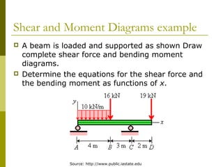
7. Shear and Moment Diagrams example
 We start by drawing a
free-body diagram of
the beam and
determining the
support reactions.
 Summing moments
about the left end of
the beam
 Summing vertical
forces
[ ] ( ) ( )
kNR
RcM
c
A
45
019916410427
=⇒
=−−⋅−=∑
Source: http://www.public.iastate.edu
( )
kNR
RRF
A
CA
30
01916104
=⇒
=−−⋅−+=∑
[ ] ( ) ( )
kNR
RcM
c
A
45
019916410427
=⇒
=−−⋅−=∑

8. Shear and Moment Diagrams example
 Sometimes knowing
the maximum and
minimum values of
the shear and bending
moment are enough
 So we will determine
shear force diagrams
by inspection
Source: http://www.public.iastate.edu

9. Shear and Moment Diagrams example
 The 30-kN support
reaction at the left end
of the beam causes
the shear force graph
to jump up 30 kN
(from 0 kN to 30 kN).
Source: http://www.public.iastate.edu

10. Shear and Moment Diagrams example
 The distributed load causes
the shear force graph to
slope downward. Since the
distributed load is
constant, the slope of the
shear force graph is
constant (dV/dx = w =
constant).
 The total change in the
shear force graph between
points A and B is 40 kN
(equal to the area under
the distributed load
between points A and B)
from +30 kN to -10 kN.
Source: http://www.public.iastate.edu

11. Shear and Moment Diagrams example
 Where does the shear
force becomes zero?
 How much of the
distributed load will it take
to cause a change of 30
kN (from +30 kN to 0
kN)? Since the distributed
load is uniform, the area
(change in shear force) is
just 10 × b = 30, which
gives b = 3 m.
 The shear force graph
becomes zero at x = 3 m
(3 m from the beginning
of the uniform distributed
load).
Source: http://www.public.iastate.edu

12. Shear and Moment Diagrams example
 The 16-kN force at B
causes the shear force
graph to drop by 16
kN (from -10 kN to
-26 kN).
Source: http://www.public.iastate.edu

13. Shear and Moment Diagrams example
 Since there are no
loads between points
B and C, the shear
force graph is
constant (the slope
dV/dx = w = 0) at -26
kN.
Source: http://www.public.iastate.edu

14. Shear and Moment Diagrams example
 Since there are no
loads between points
B and C, the shear
force graph is
constant (the slope
dV/dx = w = 0) at -26
kN.
Source: http://www.public.iastate.edu

15. Shear and Moment Diagrams example
 The 45-kN force at C
causes the shear force
graph to jump up by
45 kN, from -26 kN to
+19 kN.
Source: http://www.public.iastate.edu

16. Shear and Moment Diagrams example
 There are no loads
between points C and
D, the shear force
graph is constant (the
slope dV/dx = w = 0)
at +19 kN.
Source: http://www.public.iastate.edu

17. Shear and Moment Diagrams example
 Now we look at the moment diagram
 Note that since there are no concentrated
moments acting on the beam, the bending
moment diagram will be continuous (i.e. no
jumps)

18. Shear and Moment Diagrams example
 The bending moment graph
starts out at zero and with a
large positive slope (since the
shear force starts out with a
large positive value and
dM/dx = V ).
 As the shear force decreases,
so does the slope of the
bending moment graph. At x
= 3 m the shear force
becomes zero and the
bending moment is at a local
maximum (dM/dx = V = 0 )
 For values of x greater than 3
m (3 < x < 4 m) the shear
force is negative and the
bending moment decreases
(dM/dx = V < 0).
Source: http://www.public.iastate.edu

19. Shear and Moment Diagrams example
 The shear force graph is linear
so the bending moment graph
is a parabola.
 The change in the bending
moment between x = 0 m and
x = 3 m is equal to the area
under the shear graph
between those two points.
 So the value of the bending
moment at x = 3 m is M = 0 +
45 = 45 kN·m.
 The change in the bending
moment between x = 3 and x
= 4 m is also equal to the area
under the shear graph
 So the value of the bending
moment at x = 4 m is M = 45
- 5 = 40 kN·m.
Source: http://www.public.iastate.edu

20. Shear and Moment Diagrams example
 The bending moment graph is
continuous at x = 4 m, but the
jump in the shear force at x = 4 m
causes the slope of the bending
moment to change suddenly from
dM/dx = V = -10 kN·m/m to
dM/dx = -26 kN·m/m.
 Since the shear force graph is
constant between x = 4 m and x =
7 m, the bending moment graph
has a constant slope between x =
4 m and x = 7 m (dM/dx = V =
-26 kN·m/m).
 The change in the bending
moment between x = 4 m and x =
7 m is equal to the area under the
shear graph between those two
points.
 The area of the rectangle is just
-26 × 3= -78 kN·m. So the value
of the bending moment at x = 7 m
is M = 40 - 78 = -38 kN·m.
Source: http://www.public.iastate.edu

21. Shear and Moment Diagrams example
 Again the bending moment graph
is continuous at x = 7 m. The
jump in the shear force at x = 7 m
causes the slope of the bending
moment to change suddenly from
dM/dx = V = -26 kN·m/m to
dM/dx = +19 kN·m/m.
 Since the shear force graph is
constant between x = 7 m and x
= 9 m, the bending moment
graph has a constant slope
between x = 7 m and x = 9 m
(dM/dx = V = +19 kN·m/m).
 The change in the bending
moment between x = 7 m and x =
9 m is equal to the area under the
shear graph between those two
points. The area of the rectangle
is just M = (+19 × 2) = +38
kN·m. So the value of the bending
moment at x = 7 m is M = -38 +
38 = 0 kN·m.
Source: http://www.public.iastate.edu