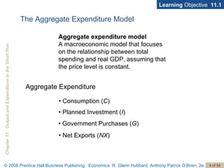
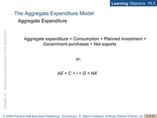
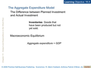
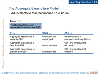
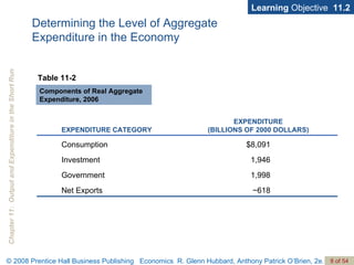
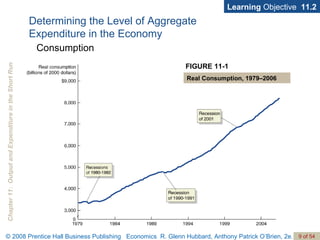
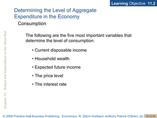
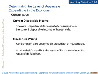
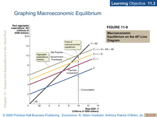
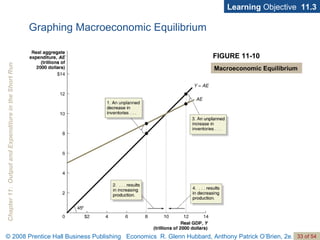
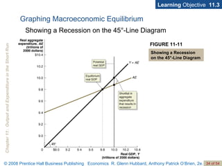
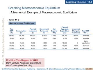
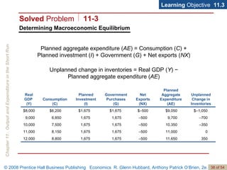
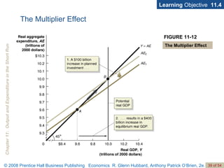
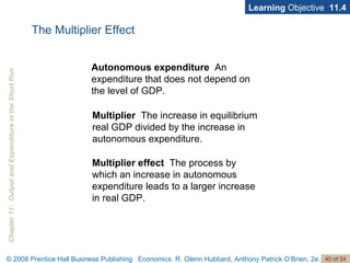
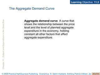
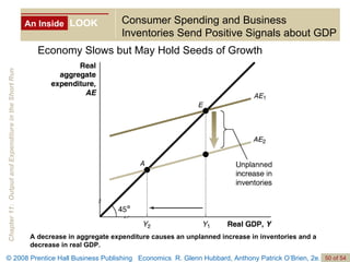
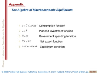
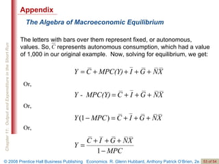
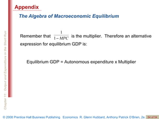
Fluctuating Demand at Cisco Systems Learning  Objectives In this chapter, we will explore the reasons for changes in aggregate expenditures and how these changes affect the level of total production in the economy. APPENDIX Apply the  algebra of macroeconomic equilibrium . Understand the relationship between the  aggregate demand curve  and aggregate expenditure. 11.5 Define the  multiplier effect  and use it to calculate changes in equilibrium GDP. 11.4 Use a  45°-line diagram  to illustrate macroeconomic equilibrium. 11.3 Discuss the determinants of the four  components of aggregate expenditure  and define the  marginal propensity to consume  and the  marginal propensity to save . 11.2 Understand how macroeconomic equilibrium is determined in the  aggregate expenditure model . 11.1
Output and Expenditure in the Short Run Aggregate expenditure ( AE )   The total amount of spending in the economy:  the sum of consumption, planned investment, government purchases, and net exports.
The Aggregate Expenditure Model Aggregate expenditure model  A macroeconomic model that focuses on the relationship between total spending and real GDP, assuming that the price level is constant. Aggregate Expenditure Learning  Objective  11.1 •  Consumption ( C ) •  Planned Investment ( I ) •  Government Purchases ( G ) •  Net Exports ( NX )
The Aggregate Expenditure Model Aggregate expenditure = Consumption + Planned investment +    Government purchases + Net exports Aggregate Expenditure Learning  Objective  11.1 or: AE = C + I + G + NX
The Aggregate Expenditure Model Inventories   Goods that have been produced but not yet sold. The Difference between Planned Investment  and Actual Investment Learning  Objective  11.1 Aggregate expenditure = GDP Macroeconomic Equilibrium
The Aggregate Expenditure Model Adjustments to Macroeconomic Equilibrium Learning  Objective  11.1 Table 11-1 The Relationship between Aggregate Expenditure and GDP GDP and employment increase . inventories fall Aggregate Expenditure is greater than GDP GDP and employment decrease. inventories rise Aggregate expenditure is less than GDP the economy is in macroeconomic equilibrium. inventories are unchanged Aggregate expenditure is equal to GDP AND … THEN … IF …
Determining the Level of Aggregate  Expenditure in the Economy Learning  Objective  11.2 Table 11-2 Components of Real Aggregate Expenditure, 2006 − 618 Net Exports 1,998 Government 1,946 Investment $8,091 Consumption EXPENDITURE (BILLIONS OF 2000 DOLLARS) EXPENDITURE CATEGORY
Determining the Level of Aggregate  Expenditure in the Economy Learning  Objective  11.2 Consumption FIGURE 11-1 Real Consumption, 1979–2006
Determining the Level of Aggregate  Expenditure in the Economy Learning  Objective  11.2 •  Current disposable income •  Household wealth •  Expected future income •  The price level •  The interest rate Consumption The following are the five most important variables that determine the level of consumption:
Determining the Level of Aggregate  Expenditure in the Economy Learning  Objective  11.2 The most important determinant of consumption is the current disposable income of households. Consumption Current Disposable Income Household Wealth Consumption also depends on the wealth of households. A household’s wealth is the value of its  assets  minus the value of its  liabilities.
Determining the Level of Aggregate  Expenditure in the Economy Learning  Objective  11.2 Consumption also depends on expected future income.  Most people prefer to keep their consumption fairly stable from year to year, even if their income fluctuates significantly.  Consumption Expected Future Income The Price Level The  price level  measures the average prices of goods and services in the economy.  Consumption is affected by changes in the price level.  The Interest Rate When the interest rate is high, the reward to saving is increased, and households are likely to save more and spend less.
Learning  Objective  11.2 FIGURE 11-2 The Relationship between  Consumption and Income, 1960– 2006 Determining the Level of Aggregate  Expenditure in the Economy Consumption The Consumption Function
Learning  Objective  11.2 Consumption function   The relationship between consumption spending and disposable income. Marginal propensity to consume ( MPC )   The slope of the consumption function:  The amount by which consumption spending changes when disposable income changes. Determining the Level of Aggregate  Expenditure in the Economy Consumption The Consumption Function
Learning  Objective  11.2 or Change in consumption = Change in disposable income ×  MPC Determining the Level of Aggregate  Expenditure in the Economy Consumption The Consumption Function We can also use the  MPC  to determine how much consumption will change as income changes:
Learning  Objective  11.2 We can rearrange the equation like this: National income = GDP = Disposable income + Net taxes Disposable income = National income − Net taxes Determining the Level of Aggregate  Expenditure in the Economy The Relationship between Consumption and National Income
Learning  Objective  11.2 FIGURE 11-2 The Relationship between  Consumption and National Income Determining the Level of Aggregate  Expenditure in the Economy The Relationship between Consumption and National Income
Learning  Objective  11.2 National income = Consumption + Saving + Taxes Change in national income = Change in consumption + Change in saving +  Change in taxes Y = C + S + T Determining the Level of Aggregate  Expenditure in the Economy Income, Consumption, and Saving and To simplify, we can assume that taxes are always a constant amount, in which case  ΔT = 0 , so the following is also true: ΔY = ΔC + ΔS
Learning  Objective  11.2 Marginal propensity to save ( MPS )  The change in saving divided by the change in disposable income. Determining the Level of Aggregate  Expenditure in the Economy Income, Consumption, and Saving or, 1  = MPC + MPS
Calculating the Marginal Propensity to  Consume and the Marginal Propensity to Save Learning  Objective  11.2 Solved  Problem 11-2 0.4 0.6 2,600 10,400 13,000 0.4 0.6 2,200 9,800 12,000 0.4 0.6 1,800 9,200 11,000 0.4 0.6 1,400 8,600 10,000 — — $1,000 $8,000 $9,000 MARGINAL PROPENSITY TO SAVE (MPS) MARGINAL PROPENSITY TO CONSUME (MPC) SAVING (S) CONSUMPTION (C) NATIONAL INCOME AND REAL GDP (Y)
Learning  Objective  11.2 FIGURE 11-4 Real Investment, 1979–2006 Determining the Level of Aggregate  Expenditure in the Economy Planned Investment
Learning  Objective  11.2 •  Expectations of future profitability •  The interest rate •  Taxes •  Cash flow Determining the Level of Aggregate  Expenditure in the Economy Planned Investment The four most important variables that determine the level of investment are:
Learning  Objective  11.2 Expectations of Future Profitability The optimism or pessimism of firms is an important determinant of investment spending. The Interest Rate A higher real interest rate results in less investment spending, and a lower real interest rate results in more investment spending. Determining the Level of Aggregate  Expenditure in the Economy Planned Investment
Determining the Level of Aggregate  Expenditure in the Economy Learning  Objective  11.2 Planned Investment Taxes Firms focus on the profits that remain after they have paid taxes. Cash Flow Cash flow   The difference between the cash revenues received by a firm and the cash spending by the firm.
Cisco Rides the Roller Coaster of Information Technology Spending Learning  Objective  11.2 Making the Connection
Learning  Objective  11.2 FIGURE 11-5 Real Government Purchases, 1979–2006 Determining the Level of Aggregate  Expenditure in the Economy Government Purchases
Learning  Objective  11.2 FIGURE 11-6 Real Net Exports, 1979–2006 Determining the Level of Aggregate  Expenditure in the Economy Net Exports
Learning  Objective  11.2 •  The price level in the United States relative to the price levels in other countries •  The growth rate of GDP in the United States relative to the growth rates of GDP in other countries •  The exchange rate between the dollar and other currencies Determining the Level of Aggregate  Expenditure in the Economy Net Exports The following are the three most important variables that determine the level of net exports:
Determining the Level of Aggregate  Expenditure in the Economy Learning  Objective  11.2 Planned Investment The Price Level in the United States Relative to the Price Levels in Other Countries If inflation in the United States is lower than inflation in other countries, prices of U.S. products increase more slowly than the prices of products of other countries. The Growth Rate of GDP in the United States Relative  to the Growth Rates of GDP in Other Countries When incomes in the United States rise more slowly than incomes in other countries, net exports will rise. The Exchange Rate Between the Dollar and Other Currencies As the value of the U.S. dollar rises, the foreign currency price of U.S. products sold in other countries rises, and the dollar price of foreign products sold in the United States falls.
Graphing Macroeconomic Equilibrium Learning  Objective  11.3 FIGURE 11-7 An Example of a  45°-Line Diagram
Learning  Objective  11.3 FIGURE 11-8 The Relationship between Planned Aggregate Expenditure and GDP on a 45°-Line Diagram Graphing Macroeconomic Equilibrium
Graphing Macroeconomic Equilibrium Learning  Objective  11.3 FIGURE 11-9 Macroeconomic Equilibrium on the 45°-Line Diagram
Learning  Objective  11.3 FIGURE 11-10 Macroeconomic Equilibrium Graphing Macroeconomic Equilibrium
Graphing Macroeconomic Equilibrium Learning  Objective  11.3 FIGURE 11-11 Showing a Recession  on the 45°-Line Diagram Showing a Recession on the 45°-Line Diagram
Graphing Macroeconomic Equilibrium Learning  Objective  11.3 Whenever planned aggregate expenditure is less than real GDP, some firms will experience an unplanned increase in inventories. The Important Role of Inventories
Business Attempts to Control Inventories, Then . . . and Now Learning  Objective  11.2 Dell Computer uses supply chain management to keep its inventory low. Making the Connection
Learning  Objective  11.3 Graphing Macroeconomic Equilibrium A Numerical Example of Macroeconomic Equilibrium Don’t Let This Happen to  YOU! Don’t Confuse Aggregate Expenditure with Consumption Spending Table 11-3 Macroeconomic Equilibrium decrease +700 11,300 – 500 1,500 1,500 8,800 12,000 decrease +350 10,650 – 500 1,500 1,500 8,150 11,000 be in equilibrium 0 10,000 – 500 1,500 1,500 7,500 10,000 increase – 350 9,350 – 500 1,500 1,500 6,850 9,000 increase – $700 $8,700 –  $500 $1,500 $1,500 $6,200 $8,000 Real GDP  Will … Unplanned Change in Inventories Planned Aggregate Expenditure (AE) Net Exports (NX) Government Purchases (G) Planned Investment (I) Consumption (C) Real GDP  (Y)
Determining Macroeconomic Equilibrium Learning  Objective  11.3 Planned aggregate expenditure ( AE ) = Consumption ( C ) + Planned investment ( I ) + Government ( G ) + Net exports ( NX ) Unplanned change in inventories = Real GDP ( Y ) − Planned aggregate expenditure ( AE ) Solved  Problem 11-3 350 11,650 – 500 1,675 1,675 8,800 12,000 0 11,000 – 500 1,675 1,675 8,150 11,000 – 350 10,350 – 500 1,675 1,675 7,500 10,000 – 700 9,700 – 500 1,675 1,675 6,850 9,000 $–1,050 $9,050 $–500 $1,675 $1,675 $6,200 $8,000 Unplanned Change in Inventories Planned Aggregate Expenditure (AE) Net Exports (NX) Government Purchases (G) Planned Investment (I) Consumption (C) Real GDP  (Y)
Learning  Objective  11.4 The Multiplier Effect FIGURE 11-12 The Multiplier Effect
Learning  Objective  11.4 The Multiplier Effect Autonomous expenditure  An expenditure that does not depend on the level of GDP. Multiplier   The increase in equilibrium real GDP divided by the increase in autonomous expenditure. Multiplier effect   The process by which an increase in autonomous expenditure leads to a larger increase in real GDP.
Learning  Objective  11.4 The Multiplier Effect Table 11-4 The Multiplier Effect in  Action 398 billion 1 billion 0 ROUND 19 $400 billion 0 0 n . . . . . . . . . . . . 395 billion 2 billion 0 ROUND 15 . . . . . . . . . . . . 377 billion 8 billion 0 ROUND 10 . . . . . . . . . . . . 305 billion 32 billion 0 ROUND 5 273 billion 42 billion 0 ROUND 4 231 billion 56 billion 0 ROUND 3 175 billion 75 billion 0 ROUND 2 $100 billion $0 $100 billion ROUND 1 TOTAL ADDITIONAL EXPENDITURE =  TOTAL ADDITIONAL GDP ADDITIONAL INDUCED EXPENDITURE (CONSUMPTION) ADDITIONAL AUTONOMOUS EXPENDITURE (INVESTMENT)  
The Multiplier in Reverse:  The Great Depression of the 1930s Learning  Objective  11.4 The multiplier effect contributed to the very high levels of unemployment during the Great Depression. Making the Connection 24.9% $636 billion -$10.2 billion $17.0 billion $541 billion 1933 3.2% $865 billion $9.4illion $91.3 billion $661 billion 1929 Unemployment Rate Real GDP Net Exports Investment Consumption Year
Learning  Objective  11.4 The Multiplier Effect A Formula for the Multiplier
Learning  Objective  11.4 The Multiplier Effect Summarizing the Multiplier Effect 1   The multiplier effect occurs both when autonomous expenditure increases and when it decreases.  2   The multiplier effect makes the economy more sensitive to changes in autonomous expenditure than it would otherwise be.  3   The larger the  MPC , the larger the value of the multiplier.  4   The formula for the multiplier, 1/(1 −  MPC ), is oversimplified because it ignores some real-world complications, such as the effect that an increasing GDP can have on imports, inflation, and interest rates.
Using the Multiplier Formula Learning  Objective  11.4 Solved  Problem 11-4 – 500 1,000 1,000 10,100 12,000 – 500 1,000 1,000 9,300 11,000 – 500 1,000 1,000 8,500 10,000 – 500 1,000 1,000 7,700 9,000 – $500 $1,000 $1,000 $6,900 $8,000 NET EXPORTS (NX) GOVERNMENT PURCHASES (G) PLANNED INVESTMENT (I) CONSUMPTION (C) REAL GDP  (Y)
Using the Multiplier Formula (continued) Learning  Objective  11.4 Solved  Problem 11-4 11,600 – 500 1,000 1,000 10,100 12,000 10,800 – 500 1,000 1,000 9,300 11,000 10,000 – 500 1,000 1,000 8,500 10,000 9,200 – 500 1,000 1,000 7,700 9,000 $8,400 – $500 $1,000 $1,000 $6,900 $8,000 PLANNED  AGGREGATE  EXPENDITURE (AE) NET EXPORTS (NX) GOVERNMENT PURCHASES (G) PLANNED INVESTMENT (I) CONSUMPTION (C) REALGDP  (Y)
Learning  Objective  11.5 The Aggregate Demand Curve FIGURE 11-13 The Effect of a Change in the Price Level on Real GDP
Learning  Objective  11.5 The Aggregate Demand Curve FIGURE 11-14 The Aggregate Demand Curve
Learning  Objective  11.5 The Aggregate Demand Curve Aggregate demand curve   A curve that shows the relationship between the price level and the level of planned aggregate expenditure in the economy, holding constant all other factors that affect aggregate expenditure.
An Inside LOOK Consumer Spending and Business Inventories Send Positive Signals about GDP Economy Slows but May Hold Seeds of Growth A decrease in aggregate expenditure causes an unplanned increase in inventories and a decrease in real GDP.
Aggregate demand curve Aggregate expenditure (AE) Aggregate expenditure model Autonomous expenditure Cash flow Consumption function Inventories Marginal propensity to consume (MPC) Marginal propensity to  save (MPS) Multiplier Multiplier effect K e y  T e r m s
The Algebra of Macroeconomic Equilibrium Appendix 1    Consumption function 2    Planned investment function 3    Government spending function 4     Net export function 5     Equilibrium condition
The Algebra of Macroeconomic Equilibrium Appendix Or, Or, Or, The letters with bars over them represent fixed, or autonomous, values. So,  represents autonomous consumption, which had a value of 1,000 in our original example.  Now, solving for equilibrium, we get:
The Algebra of Macroeconomic Equilibrium Equilibrium GDP = Autonomous expenditure x Multiplier Appendix Remember that  is the multiplier.  Therefore an alternative expression for equilibrium GDP is:

Chap11pp

  • 1.
  • 2.
    Fluctuating Demand atCisco Systems Learning Objectives In this chapter, we will explore the reasons for changes in aggregate expenditures and how these changes affect the level of total production in the economy. APPENDIX Apply the algebra of macroeconomic equilibrium . Understand the relationship between the aggregate demand curve and aggregate expenditure. 11.5 Define the multiplier effect and use it to calculate changes in equilibrium GDP. 11.4 Use a 45°-line diagram to illustrate macroeconomic equilibrium. 11.3 Discuss the determinants of the four components of aggregate expenditure and define the marginal propensity to consume and the marginal propensity to save . 11.2 Understand how macroeconomic equilibrium is determined in the aggregate expenditure model . 11.1
  • 3.
    Output and Expenditurein the Short Run Aggregate expenditure ( AE ) The total amount of spending in the economy: the sum of consumption, planned investment, government purchases, and net exports.
  • 4.
    The Aggregate ExpenditureModel Aggregate expenditure model A macroeconomic model that focuses on the relationship between total spending and real GDP, assuming that the price level is constant. Aggregate Expenditure Learning Objective 11.1 • Consumption ( C ) • Planned Investment ( I ) • Government Purchases ( G ) • Net Exports ( NX )
  • 5.
    The Aggregate ExpenditureModel Aggregate expenditure = Consumption + Planned investment + Government purchases + Net exports Aggregate Expenditure Learning Objective 11.1 or: AE = C + I + G + NX
  • 6.
    The Aggregate ExpenditureModel Inventories Goods that have been produced but not yet sold. The Difference between Planned Investment and Actual Investment Learning Objective 11.1 Aggregate expenditure = GDP Macroeconomic Equilibrium
  • 7.
    The Aggregate ExpenditureModel Adjustments to Macroeconomic Equilibrium Learning Objective 11.1 Table 11-1 The Relationship between Aggregate Expenditure and GDP GDP and employment increase . inventories fall Aggregate Expenditure is greater than GDP GDP and employment decrease. inventories rise Aggregate expenditure is less than GDP the economy is in macroeconomic equilibrium. inventories are unchanged Aggregate expenditure is equal to GDP AND … THEN … IF …
  • 8.
    Determining the Levelof Aggregate Expenditure in the Economy Learning Objective 11.2 Table 11-2 Components of Real Aggregate Expenditure, 2006 − 618 Net Exports 1,998 Government 1,946 Investment $8,091 Consumption EXPENDITURE (BILLIONS OF 2000 DOLLARS) EXPENDITURE CATEGORY
  • 9.
    Determining the Levelof Aggregate Expenditure in the Economy Learning Objective 11.2 Consumption FIGURE 11-1 Real Consumption, 1979–2006
  • 10.
    Determining the Levelof Aggregate Expenditure in the Economy Learning Objective 11.2 • Current disposable income • Household wealth • Expected future income • The price level • The interest rate Consumption The following are the five most important variables that determine the level of consumption:
  • 11.
    Determining the Levelof Aggregate Expenditure in the Economy Learning Objective 11.2 The most important determinant of consumption is the current disposable income of households. Consumption Current Disposable Income Household Wealth Consumption also depends on the wealth of households. A household’s wealth is the value of its assets minus the value of its liabilities.
  • 12.
    Determining the Levelof Aggregate Expenditure in the Economy Learning Objective 11.2 Consumption also depends on expected future income. Most people prefer to keep their consumption fairly stable from year to year, even if their income fluctuates significantly. Consumption Expected Future Income The Price Level The price level measures the average prices of goods and services in the economy. Consumption is affected by changes in the price level. The Interest Rate When the interest rate is high, the reward to saving is increased, and households are likely to save more and spend less.
  • 13.
    Learning Objective 11.2 FIGURE 11-2 The Relationship between Consumption and Income, 1960– 2006 Determining the Level of Aggregate Expenditure in the Economy Consumption The Consumption Function
  • 14.
    Learning Objective 11.2 Consumption function The relationship between consumption spending and disposable income. Marginal propensity to consume ( MPC ) The slope of the consumption function: The amount by which consumption spending changes when disposable income changes. Determining the Level of Aggregate Expenditure in the Economy Consumption The Consumption Function
  • 15.
    Learning Objective 11.2 or Change in consumption = Change in disposable income × MPC Determining the Level of Aggregate Expenditure in the Economy Consumption The Consumption Function We can also use the MPC to determine how much consumption will change as income changes:
  • 16.
    Learning Objective 11.2 We can rearrange the equation like this: National income = GDP = Disposable income + Net taxes Disposable income = National income − Net taxes Determining the Level of Aggregate Expenditure in the Economy The Relationship between Consumption and National Income
  • 17.
    Learning Objective 11.2 FIGURE 11-2 The Relationship between Consumption and National Income Determining the Level of Aggregate Expenditure in the Economy The Relationship between Consumption and National Income
  • 18.
    Learning Objective 11.2 National income = Consumption + Saving + Taxes Change in national income = Change in consumption + Change in saving + Change in taxes Y = C + S + T Determining the Level of Aggregate Expenditure in the Economy Income, Consumption, and Saving and To simplify, we can assume that taxes are always a constant amount, in which case ΔT = 0 , so the following is also true: ΔY = ΔC + ΔS
  • 19.
    Learning Objective 11.2 Marginal propensity to save ( MPS ) The change in saving divided by the change in disposable income. Determining the Level of Aggregate Expenditure in the Economy Income, Consumption, and Saving or, 1 = MPC + MPS
  • 20.
    Calculating the MarginalPropensity to Consume and the Marginal Propensity to Save Learning Objective 11.2 Solved Problem 11-2 0.4 0.6 2,600 10,400 13,000 0.4 0.6 2,200 9,800 12,000 0.4 0.6 1,800 9,200 11,000 0.4 0.6 1,400 8,600 10,000 — — $1,000 $8,000 $9,000 MARGINAL PROPENSITY TO SAVE (MPS) MARGINAL PROPENSITY TO CONSUME (MPC) SAVING (S) CONSUMPTION (C) NATIONAL INCOME AND REAL GDP (Y)
  • 21.
    Learning Objective 11.2 FIGURE 11-4 Real Investment, 1979–2006 Determining the Level of Aggregate Expenditure in the Economy Planned Investment
  • 22.
    Learning Objective 11.2 • Expectations of future profitability • The interest rate • Taxes • Cash flow Determining the Level of Aggregate Expenditure in the Economy Planned Investment The four most important variables that determine the level of investment are:
  • 23.
    Learning Objective 11.2 Expectations of Future Profitability The optimism or pessimism of firms is an important determinant of investment spending. The Interest Rate A higher real interest rate results in less investment spending, and a lower real interest rate results in more investment spending. Determining the Level of Aggregate Expenditure in the Economy Planned Investment
  • 24.
    Determining the Levelof Aggregate Expenditure in the Economy Learning Objective 11.2 Planned Investment Taxes Firms focus on the profits that remain after they have paid taxes. Cash Flow Cash flow The difference between the cash revenues received by a firm and the cash spending by the firm.
  • 25.
    Cisco Rides theRoller Coaster of Information Technology Spending Learning Objective 11.2 Making the Connection
  • 26.
    Learning Objective 11.2 FIGURE 11-5 Real Government Purchases, 1979–2006 Determining the Level of Aggregate Expenditure in the Economy Government Purchases
  • 27.
    Learning Objective 11.2 FIGURE 11-6 Real Net Exports, 1979–2006 Determining the Level of Aggregate Expenditure in the Economy Net Exports
  • 28.
    Learning Objective 11.2 • The price level in the United States relative to the price levels in other countries • The growth rate of GDP in the United States relative to the growth rates of GDP in other countries • The exchange rate between the dollar and other currencies Determining the Level of Aggregate Expenditure in the Economy Net Exports The following are the three most important variables that determine the level of net exports:
  • 29.
    Determining the Levelof Aggregate Expenditure in the Economy Learning Objective 11.2 Planned Investment The Price Level in the United States Relative to the Price Levels in Other Countries If inflation in the United States is lower than inflation in other countries, prices of U.S. products increase more slowly than the prices of products of other countries. The Growth Rate of GDP in the United States Relative to the Growth Rates of GDP in Other Countries When incomes in the United States rise more slowly than incomes in other countries, net exports will rise. The Exchange Rate Between the Dollar and Other Currencies As the value of the U.S. dollar rises, the foreign currency price of U.S. products sold in other countries rises, and the dollar price of foreign products sold in the United States falls.
  • 30.
    Graphing Macroeconomic EquilibriumLearning Objective 11.3 FIGURE 11-7 An Example of a 45°-Line Diagram
  • 31.
    Learning Objective 11.3 FIGURE 11-8 The Relationship between Planned Aggregate Expenditure and GDP on a 45°-Line Diagram Graphing Macroeconomic Equilibrium
  • 32.
    Graphing Macroeconomic EquilibriumLearning Objective 11.3 FIGURE 11-9 Macroeconomic Equilibrium on the 45°-Line Diagram
  • 33.
    Learning Objective 11.3 FIGURE 11-10 Macroeconomic Equilibrium Graphing Macroeconomic Equilibrium
  • 34.
    Graphing Macroeconomic EquilibriumLearning Objective 11.3 FIGURE 11-11 Showing a Recession on the 45°-Line Diagram Showing a Recession on the 45°-Line Diagram
  • 35.
    Graphing Macroeconomic EquilibriumLearning Objective 11.3 Whenever planned aggregate expenditure is less than real GDP, some firms will experience an unplanned increase in inventories. The Important Role of Inventories
  • 36.
    Business Attempts toControl Inventories, Then . . . and Now Learning Objective 11.2 Dell Computer uses supply chain management to keep its inventory low. Making the Connection
  • 37.
    Learning Objective 11.3 Graphing Macroeconomic Equilibrium A Numerical Example of Macroeconomic Equilibrium Don’t Let This Happen to YOU! Don’t Confuse Aggregate Expenditure with Consumption Spending Table 11-3 Macroeconomic Equilibrium decrease +700 11,300 – 500 1,500 1,500 8,800 12,000 decrease +350 10,650 – 500 1,500 1,500 8,150 11,000 be in equilibrium 0 10,000 – 500 1,500 1,500 7,500 10,000 increase – 350 9,350 – 500 1,500 1,500 6,850 9,000 increase – $700 $8,700 – $500 $1,500 $1,500 $6,200 $8,000 Real GDP Will … Unplanned Change in Inventories Planned Aggregate Expenditure (AE) Net Exports (NX) Government Purchases (G) Planned Investment (I) Consumption (C) Real GDP (Y)
  • 38.
    Determining Macroeconomic EquilibriumLearning Objective 11.3 Planned aggregate expenditure ( AE ) = Consumption ( C ) + Planned investment ( I ) + Government ( G ) + Net exports ( NX ) Unplanned change in inventories = Real GDP ( Y ) − Planned aggregate expenditure ( AE ) Solved Problem 11-3 350 11,650 – 500 1,675 1,675 8,800 12,000 0 11,000 – 500 1,675 1,675 8,150 11,000 – 350 10,350 – 500 1,675 1,675 7,500 10,000 – 700 9,700 – 500 1,675 1,675 6,850 9,000 $–1,050 $9,050 $–500 $1,675 $1,675 $6,200 $8,000 Unplanned Change in Inventories Planned Aggregate Expenditure (AE) Net Exports (NX) Government Purchases (G) Planned Investment (I) Consumption (C) Real GDP (Y)
  • 39.
    Learning Objective 11.4 The Multiplier Effect FIGURE 11-12 The Multiplier Effect
  • 40.
    Learning Objective 11.4 The Multiplier Effect Autonomous expenditure An expenditure that does not depend on the level of GDP. Multiplier The increase in equilibrium real GDP divided by the increase in autonomous expenditure. Multiplier effect The process by which an increase in autonomous expenditure leads to a larger increase in real GDP.
  • 41.
    Learning Objective 11.4 The Multiplier Effect Table 11-4 The Multiplier Effect in Action 398 billion 1 billion 0 ROUND 19 $400 billion 0 0 n . . . . . . . . . . . . 395 billion 2 billion 0 ROUND 15 . . . . . . . . . . . . 377 billion 8 billion 0 ROUND 10 . . . . . . . . . . . . 305 billion 32 billion 0 ROUND 5 273 billion 42 billion 0 ROUND 4 231 billion 56 billion 0 ROUND 3 175 billion 75 billion 0 ROUND 2 $100 billion $0 $100 billion ROUND 1 TOTAL ADDITIONAL EXPENDITURE = TOTAL ADDITIONAL GDP ADDITIONAL INDUCED EXPENDITURE (CONSUMPTION) ADDITIONAL AUTONOMOUS EXPENDITURE (INVESTMENT)  
  • 42.
    The Multiplier inReverse: The Great Depression of the 1930s Learning Objective 11.4 The multiplier effect contributed to the very high levels of unemployment during the Great Depression. Making the Connection 24.9% $636 billion -$10.2 billion $17.0 billion $541 billion 1933 3.2% $865 billion $9.4illion $91.3 billion $661 billion 1929 Unemployment Rate Real GDP Net Exports Investment Consumption Year
  • 43.
    Learning Objective 11.4 The Multiplier Effect A Formula for the Multiplier
  • 44.
    Learning Objective 11.4 The Multiplier Effect Summarizing the Multiplier Effect 1 The multiplier effect occurs both when autonomous expenditure increases and when it decreases. 2 The multiplier effect makes the economy more sensitive to changes in autonomous expenditure than it would otherwise be. 3 The larger the MPC , the larger the value of the multiplier. 4 The formula for the multiplier, 1/(1 − MPC ), is oversimplified because it ignores some real-world complications, such as the effect that an increasing GDP can have on imports, inflation, and interest rates.
  • 45.
    Using the MultiplierFormula Learning Objective 11.4 Solved Problem 11-4 – 500 1,000 1,000 10,100 12,000 – 500 1,000 1,000 9,300 11,000 – 500 1,000 1,000 8,500 10,000 – 500 1,000 1,000 7,700 9,000 – $500 $1,000 $1,000 $6,900 $8,000 NET EXPORTS (NX) GOVERNMENT PURCHASES (G) PLANNED INVESTMENT (I) CONSUMPTION (C) REAL GDP (Y)
  • 46.
    Using the MultiplierFormula (continued) Learning Objective 11.4 Solved Problem 11-4 11,600 – 500 1,000 1,000 10,100 12,000 10,800 – 500 1,000 1,000 9,300 11,000 10,000 – 500 1,000 1,000 8,500 10,000 9,200 – 500 1,000 1,000 7,700 9,000 $8,400 – $500 $1,000 $1,000 $6,900 $8,000 PLANNED AGGREGATE EXPENDITURE (AE) NET EXPORTS (NX) GOVERNMENT PURCHASES (G) PLANNED INVESTMENT (I) CONSUMPTION (C) REALGDP (Y)
  • 47.
    Learning Objective 11.5 The Aggregate Demand Curve FIGURE 11-13 The Effect of a Change in the Price Level on Real GDP
  • 48.
    Learning Objective 11.5 The Aggregate Demand Curve FIGURE 11-14 The Aggregate Demand Curve
  • 49.
    Learning Objective 11.5 The Aggregate Demand Curve Aggregate demand curve A curve that shows the relationship between the price level and the level of planned aggregate expenditure in the economy, holding constant all other factors that affect aggregate expenditure.
  • 50.
    An Inside LOOKConsumer Spending and Business Inventories Send Positive Signals about GDP Economy Slows but May Hold Seeds of Growth A decrease in aggregate expenditure causes an unplanned increase in inventories and a decrease in real GDP.
  • 51.
    Aggregate demand curveAggregate expenditure (AE) Aggregate expenditure model Autonomous expenditure Cash flow Consumption function Inventories Marginal propensity to consume (MPC) Marginal propensity to save (MPS) Multiplier Multiplier effect K e y T e r m s
  • 52.
    The Algebra ofMacroeconomic Equilibrium Appendix 1 Consumption function 2 Planned investment function 3 Government spending function 4 Net export function 5 Equilibrium condition
  • 53.
    The Algebra ofMacroeconomic Equilibrium Appendix Or, Or, Or, The letters with bars over them represent fixed, or autonomous, values. So, represents autonomous consumption, which had a value of 1,000 in our original example. Now, solving for equilibrium, we get:
  • 54.
    The Algebra ofMacroeconomic Equilibrium Equilibrium GDP = Autonomous expenditure x Multiplier Appendix Remember that is the multiplier. Therefore an alternative expression for equilibrium GDP is: