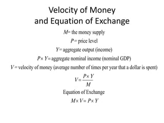
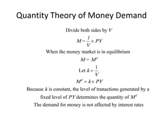
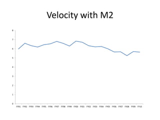
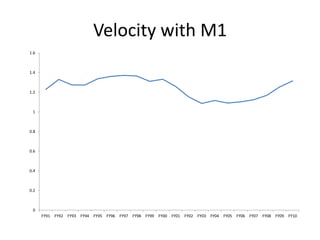
This document provides an overview of the quantity theory of money. It discusses the history of the theory as outlined by Irving Fisher in 1911. Fisher examined the link between the money supply (M), price level (P), and aggregate output or income (Y). This relationship is captured in the equation of exchange: M × V = P × Y, where V is the velocity of money, or how quickly money circulates in the economy. The document then explains that according to the quantity theory, changes in the money supply will only affect the price level as long as velocity and output remain constant in the short run. Finally, it provides graphs showing how velocity has changed over time for different monetary aggregates in Egypt.
1. Quantity Theory of Money
Chahir Zaki
FEPS, Cairo University
Second semester, 2012
2. Outline
1. Introduction
2. History
3. Velocity
4. Quantity Theory of Money
5. Velocity in Egypt
3. Outline
1. Introduction
2. History
3. Velocity
4. Quantity Theory of Money
5. Velocity in Egypt
4. Introduction
• The quantity theory of money is a theory of how the
nominal value of aggregate income is determined.
• Because it also tells us how much money is held for a
given amount of aggregate income, it is also a theory
of the demand for money.
• The most important feature of this theory is that it
suggests that interest rates have no effect on the
demand for money.
5. Outline
1. Introduction
2. History
3. Velocity
4. Quantity Theory of Money
5. Velocity in Egypt
6. History
•The clearest exposition of the classical quantity theory
approach is found in the work of the American
economist Irving Fisher, in his influential book The
Purchasing Power of Money, published in 1911.
•Fisher wanted to examine the link between the total
quantity of money M (the money supply) and the total
amount of spending on final goods and services
produced in the economy P Y, where P is the price level
and Y is aggregate output (income or nominal GDP.)
7. Outline
1. Introduction
2. History
3. Velocity
4. Quantity Theory of Money
5. Velocity in Egypt
8. Velocity of Money
and Equation of Exchange
M = the money supply
P = price level
Y = aggregate output (income)
P Y aggregate nominal income (nominal GDP)
V = velocity of money (average number of times per year that a dollar is spent)
P Y
V
M
Equation of Exchange
M V P Y
9. Velocity of Money
• The concept that provides the link between M
and P , Y is called the velocity of money:
• The rate of turnover of money
• The average number of times per year that a
dollar is spent in buying the total amount of
goods and services produced in the economy.
10. Velocity of Money
• Irving Fisher reasoned that velocity is determined by the
institutions in an economy that affect the way individuals
conduct transactions.
• If people use charge accounts and credit cards to conduct
their transactions and consequently use money less often
when making purchases, less money is required to conduct
the transactions generated by nominal income (M↓ relative
to P Y), and velocity (P Y )/M will increase.
• Conversely, if it is more convenient for purchases to be
paid for with cash or checks (both of which are money),
more money is used to conduct the transactions generated
by the same level of nominal income, and velocity will fall.
11. Outline
1. Introduction
2. History
3. Velocity
4. Quantity Theory of Money
5. Velocity in Egypt
12. Quantity Theory
• Velocity fairly constant in short run
• Aggregate output at full-employment level
• Changes in money supply affect only the price level
• Movement in the price level results solely from change
in the quantity of money
13. Quantity Theory of Money Demand
Divide both sides by V
1
M = PY
V
When the money market is in equilibrium
M = Md
1
Let k
V
M d k PY
Because k is constant, the level of tranactions generated by a
fixed level of PY determines the quantity of M d
The demand for money is not affected by interest rates
14. Outline
1. Introduction
2. History
3. Velocity
4. Quantity Theory of Money
5. Velocity in Egypt