Downloaded 293 times
![Project Management for Construction: Cost Estimation http://pmbook.ce.cmu.edu/05_Cost_Estimation.html
Insurance and taxes
Financing costs
Utilities
Owner's other expenses
The magnitude of each of these cost components depends on the nature, size and location of the project as
well as the management organization, among many considerations. The owner is interested in achieving the
lowest possible overall project cost that is consistent with its investment objectives.
It is important for design professionals and construction managers to realize that while the construction cost
may be the single largest component of the capital cost, other cost components are not insignificant. For
example, land acquisition costs are a major expenditure for building construction in high-density urban areas,
and construction financing costs can reach the same order of magnitude as the construction cost in large
projects such as the construction of nuclear power plants.
From the owner's perspective, it is equally important to estimate the corresponding operation and maintenance
cost of each alternative for a proposed facility in order to analyze the life cycle costs. The large expenditures
needed for facility maintenance, especially for publicly owned infrastructure, are reminders of the neglect in
the past to consider fully the implications of operation and maintenance cost in the design stage.
In most construction budgets, there is an allowance for contingencies or unexpected costs occuring during
construction. This contingency amount may be included within each cost item or be included in a single
category of construction contingency. The amount of contingency is based on historical experience and the
expected difficulty of a particular construction project. For example, one construction firm makes estimates of
the expected cost in five different areas:
Design development changes,
Schedule adjustments,
General administration changes (such as wage rates),
Differing site conditions for those expected, and
Third party requirements imposed during construction, such as new permits.
Contingent amounts not spent for construction can be released near the end of construction to the owner or to
add additional project elements.
In this chapter, we shall focus on the estimation of construction cost, with only occasional reference to other
cost components. In Chapter 6, we shall deal with the economic evaluation of a constructed facility on the
basis of both the capital cost and the operation and maintenance cost in the life cycle of the facility. It is at this
stage that tradeoffs between operating and capital costs can be analyzed.
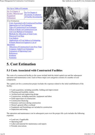
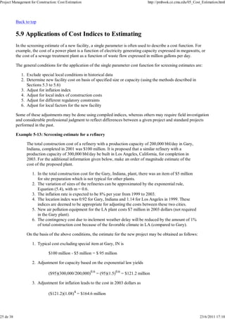
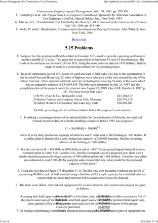
Example 5-1: Energy project resource demands [1]
The resources demands for three types of major energy projects investigated during the energy
crisis in the 1970's are shown in Table 5-1. These projects are: (1) an oil shale project with a
capacity of 50,000 barrels of oil product per day; (2) a coal gasification project that makes gas
with a heating value of 320 billions of British thermal units per day, or equivalent to about 50,000
barrels of oil product per day; and (3) a tar sand project with a capacity of 150,000 barrels of oil
product per day.
For each project, the cost in billions of dollars, the engineering manpower requirement for basic
design in thousands of hours, the engineering manpower requirement for detailed engineering in
millions of hours, the skilled labor requirement for construction in millions of hours and the
material requirement in billions of dollars are shown in Table 5-1. To build several projects of
such an order of magnitude concurrently could drive up the costs and strain the availability of all
resources required to complete the projects. Consequently, cost estimation often represents an
exercise in professional judgment instead of merely compiling a bill of quantities and collecting
cost data to reach a total estimate mechanically.
2 de 38 23/6/2011 17:10](https://image.slidesharecdn.com/5-costestimation-110716160453-phpapp01/85/5-cost-estimation-2-320.jpg)
![Project Management for Construction: Cost Estimation http://pmbook.ce.cmu.edu/05_Cost_Estimation.html
work is clearly defined and the detailed design is in progress so that the essential features of the facility are
identifiable. The engineer's estimate is based on the completed plans and specifications when they are ready
for the owner to solicit bids from construction contractors. In preparing these estimates, the design
professional will include expected amounts for contractors' overhead and profits.
The costs associated with a facility may be decomposed into a hierarchy of levels that are appropriate for the
purpose of cost estimation. The level of detail in decomposing the facility into tasks depends on the type of
cost estimate to be prepared. For conceptual estimates, for example, the level of detail in defining tasks is
quite coarse; for detailed estimates, the level of detail can be quite fine.
As an example, consider the cost estimates for a proposed bridge across a river. A screening estimate is made
for each of the potential alternatives, such as a tied arch bridge or a cantilever truss bridge. As the bridge type
is selected, e.g. the technology is chosen to be a tied arch bridge instead of some new bridge form, a
preliminary estimate is made on the basis of the layout of the selected bridge form on the basis of the
preliminary or conceptual design. When the detailed design has progressed to a point when the essential
details are known, a detailed estimate is made on the basis of the well defined scope of the project. When the
detailed plans and specifications are completed, an engineer's estimate can be made on the basis of items and
quantities of work.
Bid Estimates
The contractor's bid estimates often reflect the desire of the contractor to secure the job as well as the
estimating tools at its disposal. Some contractors have well established cost estimating procedures while others
do not. Since only the lowest bidder will be the winner of the contract in most bidding contests, any effort
devoted to cost estimating is a loss to the contractor who is not a successful bidder. Consequently, the
contractor may put in the least amount of possible effort for making a cost estimate if it believes that its
chance of success is not high.
If a general contractor intends to use subcontractors in the construction of a facility, it may solicit price
quotations for various tasks to be subcontracted to specialty subcontractors. Thus, the general subcontractor
will shift the burden of cost estimating to subcontractors. If all or part of the construction is to be undertaken
by the general contractor, a bid estimate may be prepared on the basis of the quantity takeoffs from the plans
provided by the owner or on the basis of the construction procedures devised by the contractor for
implementing the project. For example, the cost of a footing of a certain type and size may be found in
commercial publications on cost data which can be used to facilitate cost estimates from quantity takeoffs.
However, the contractor may want to assess the actual cost of construction by considering the actual
construction procedures to be used and the associated costs if the project is deemed to be different from
typical designs. Hence, items such as labor, material and equipment needed to perform various tasks may be
used as parameters for the cost estimates.
Control Estimates
Both the owner and the contractor must adopt some base line for cost control during the construction. For the
owner, a budget estimate must be adopted early enough for planning long term financing of the facility.
Consequently, the detailed estimate is often used as the budget estimate since it is sufficient definitive to
reflect the project scope and is available long before the engineer's estimate. As the work progresses, the
budgeted cost must be revised periodically to reflect the estimated cost to completion. A revised estimated
cost is necessary either because of change orders initiated by the owner or due to unexpected cost overruns or
savings.
For the contractor, the bid estimate is usually regarded as the budget estimate, which will be used for control
purposes as well as for planning construction financing. The budgeted cost should also be updated periodically
to reflect the estimated cost to completion as well as to insure adequate cash flows for the completion of the
project.
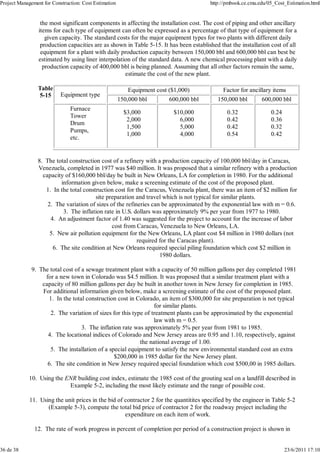
Example 5-2: Screening estimate of a grouting seal beneath a landfill [2]
5 de 38 23/6/2011 17:10](https://image.slidesharecdn.com/5-costestimation-110716160453-phpapp01/85/5-cost-estimation-5-320.jpg)
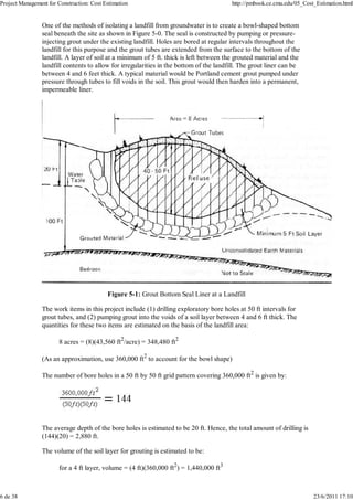
![Project Management for Construction: Cost Estimation http://pmbook.ce.cmu.edu/05_Cost_Estimation.html
for a 6 ft layer, volume = (6 ft)(360,000 ft2) = 2,160,000 ft3
It is estimated from soil tests that the voids in the soil layer are between 20% and 30% of the total
volume. Thus, for a 4 ft soil layer:
grouting in 20% voids = (20%)(1,440,000) = 288,000 ft3
grouting in 30 % voids = (30%)(1,440,000) = 432,000 ft3
and for a 6 ft soil layer:
grouting in 20% voids = (20%)(2,160,000) = 432,000 ft3
grouting in 30% voids = (30%)(2,160,000) = 648,000 ft3
The unit cost for drilling exploratory bore holes is estimated to be between $3 and $10 per foot (in
1978 dollars) including all expenses. Thus, the total cost of boring will be between (2,880)(3) = $
8,640 and (2,880)(10) = $28,800. The unit cost of Portland cement grout pumped into place is
between $4 and $10 per cubic foot including overhead and profit. In addition to the variation in
the unit cost, the total cost of the bottom seal will depend upon the thickness of the soil layer
grouted and the proportion of voids in the soil. That is:
for a 4 ft layer with 20% voids, grouting cost = $1,152,000 to $2,880,000
for a 4 ft layer with 30% voids, grouting cost = $1,728,000 to $4,320,000
for a 6 ft layer with 20% voids, grouting cost = $1,728,000 to $4,320,000
for a 6 ft layer with 30% voids, grouting cost = $2,592,000 to $6,480,000
The total cost of drilling bore holes is so small in comparison with the cost of grouting that the
former can be omitted in the screening estimate. Furthermore, the range of unit cost varies greatly
with soil characteristics, and the engineer must exercise judgment in narrowing the range of the
total cost. Alternatively, additional soil tests can be used to better estimate the unit cost of
pumping grout and the proportion of voids in the soil. Suppose that, in addition to ignoring the
cost of bore holes, an average value of a 5 ft soil layer with 25% voids is used together with a unit
cost of $ 7 per cubic foot of Portland cement grouting. In this case, the total project cost is
estimated to be:
(5 ft)(360,000 ft2)(25%)($7/ft3) = $3,150,000
An important point to note is that this screening estimate is based to a large degree on engineering
judgment of the soil characteristics, and the range of the actual cost may vary from $ 1,152,000 to
$ 6,480,000 even though the probabilities of having actual costs at the extremes are not very high.
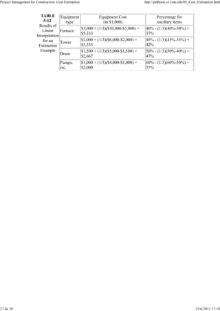
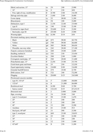
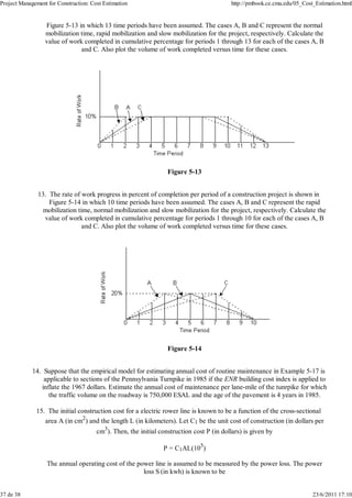
Example 5-3: Example of engineer's estimate and contractors' bids[3]
The engineer's estimate for a project involving 14 miles of Interstate 70 roadway in Utah was
$20,950,859. Bids were submitted on March 10, 1987, for completing the project within 320
working days. The three low bidders were:
1. Ball, Ball & Brosame, Inc.,
$14,129,798
Danville CA
2. National Projects, Inc., Phoenix,
$15,381,789
AR
3. Kiewit Western Co., Murray, Utah $18,146,714
It was astounding that the winning bid was 32% below the engineer's estimate. Even the third
lowest bidder was 13% below the engineer's estimate for this project. The disparity in pricing can
be attributed either to the very conservative estimate of the engineer in the Utah Department of
7 de 38 23/6/2011 17:10](https://image.slidesharecdn.com/5-costestimation-110716160453-phpapp01/85/5-cost-estimation-7-320.jpg)
![Project Management for Construction: Cost Estimation http://pmbook.ce.cmu.edu/05_Cost_Estimation.html
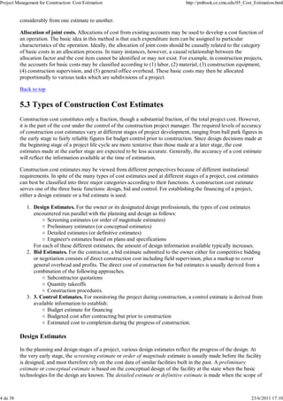
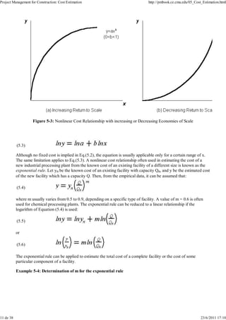
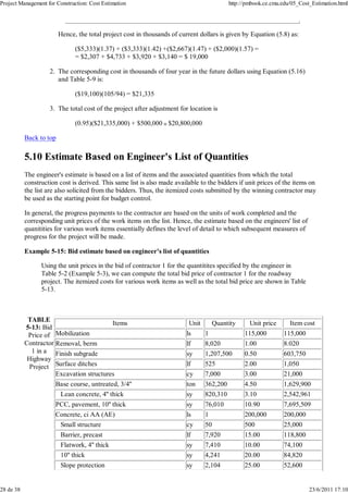
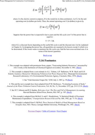
Figure 5-4: Log-Log Scale Graph of Exponential Rule Example
The empirical cost data from a number of sewage treatment plants are plotted on a log-log scale
for ln(Q/Qn) and ln(y/yn) and a linear relationship between these logarithmic ratios is shown in
Figure 5-4. For (Q/Qn) = 1 or ln(Q/Qn) = 0, ln(y/yn) = 0; and for Q/Qn = 2 or ln(Q/Qn) = 0.301,
ln(y/yn) = 0.1765. Since m is the slope of the line in the figure, it can be determined from the
geometric relation as follows:
For ln(y/yn) = 0.1765, y/yn = 1.5, while the corresponding value of Q/Qn is 2. In words, for m =
0.585, the cost of a plant increases only 1.5 times when the capacity is doubled.
Example 5-5: Cost exponents for water and wastewater treatment plants[4]
The magnitude of the cost exponent m in the exponential rule provides a simple measure of the
economy of scale associated with building extra capacity for future growth and system reliability
for the present in the design of treatment plants. When m is small, there is considerable incentive
to provide extra capacity since scale economies exist as illustrated in Figure 5-3. When m is close
to 1, the cost is directly proportional to the design capacity. The value of m tends to increase as
the number of duplicate units in a system increases. The values of m for several types of
treatment plants with different plant components derived from statistical correlation of actual
construction costs are shown in Table 5-3.
TABLE
5-3 Treatment plant Exponent Capacity range
Estimated type m (millions of gallons per day)
Values of
Cost
Exponents 1. Water treatment 0.67 1-100
for Water 2. Waste treatment
Treatment Primary with digestion (small) 0.55 0.1-10
Plants Primary with digestion (large) 0.75 0.7-100
Trickling filter 0.60 0.1-20
Activated sludge 0.77 0.1-100
Stabilization ponds 0.57 0.1-100
12 de 38 23/6/2011 17:10](https://image.slidesharecdn.com/5-costestimation-110716160453-phpapp01/85/5-cost-estimation-12-320.jpg)
![Project Management for Construction: Cost Estimation http://pmbook.ce.cmu.edu/05_Cost_Estimation.html
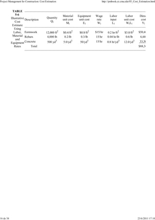
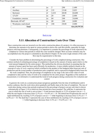
Example 5-10: A standard cost report for allocating overhead
The reliance on labor expenses as a means of allocating overhead burdens in typical management
accounting systems can be illustrated by the example of a particular product's standard cost
sheet. [5] Table 5-8 is an actual product's standard cost sheet of a company following the
procedure of using overhead burden rates assessed per direct labor hour. The material and labor
costs for manufacturing a type of valve were estimated from engineering studies and from current
material and labor prices. These amounts are summarized in Columns 2 and 3 of Table 5-8. The
overhead costs shown in Column 4 of Table 5-8 were obtained by allocating the expenses of
several departments to the various products manufactured in these departments in proportion to
the labor cost. As shown in the last line of the table, the material cost represents 29% of the total
cost, while labor costs are 11% of the total cost. The allocated overhead cost constitutes 60% of
the total cost. Even though material costs exceed labor costs, only the labor costs are used in
allocating overhead. Although this type of allocation method is common in industry, the arbitrary
allocation of joint costs introduces unintended cross subsidies among products and may produce
adverse consequences on sales and profits. For example, a particular type of part may incur few
overhead expenses in practice, but this phenomenon would not be reflected in the standard cost
report.
TABLE
5-8 (1) Material cost (2) Labor cost (3) Overhead cost (4) Total cost
Standard
Cost
Report Purchased part $1.1980 $1.1980
for a Operation
Type of Drill, face, tap (2) $0.0438 $0.2404 $0.2842
Valve Degrease 0.0031 0.0337 0.0368
Remove burs 0.0577 0.3241 0.3818
Total cost, this item 1.1980 0.1046 0.5982 1.9008
Other subassemblies 0.3523 0.2994 1.8519 2.4766
Total cost, subassemblies 1.5233 0.4040 2.4501 4.3773
Assemble and test 0.1469 0.4987 0.6456
Pack without paper 0.0234 0.1349 0.1583
Total cost, this item $1.5233 $0.5743 $3.0837 $5.1813
Cost component, % 29% 11% 60% 100%
Source: H. T. Johnson and R. S. Kaplan, Relevance lost: The Rise and Fall of Management
Accounting, Harvard Business School Press, Boston. Reprinted with permission.
Back to top
5.7 Historical Cost Data
Preparing cost estimates normally requires the use of historical data on construction costs. Historical cost data
will be useful for cost estimation only if they are collected and organized in a way that is compatible with
future applications. Organizations which are engaged in cost estimation continually should keep a file for their
own use. The information must be updated with respect to changes that will inevitably occur. The format of
cost data, such as unit costs for various items, should be organized according to the current standard of usage
in the organization.
Construction cost data are published in various forms by a number of organizations. These publications are
useful as references for comparison. Basically, the following types of information are available:
19 de 38 23/6/2011 17:10](https://image.slidesharecdn.com/5-costestimation-110716160453-phpapp01/85/5-cost-estimation-19-320.jpg)
![Project Management for Construction: Cost Estimation http://pmbook.ce.cmu.edu/05_Cost_Estimation.html
the management of costs during construction.
Version control to allow simulation of different construction processes or design changes for the purpose
of tracking changes in expected costs.
Provisions for manual review, over-ride and editing of any cost element resulting from the cost
estimation system
Flexible reporting formats, including provisions for electronic reporting rather than simply printing cost
estimates on paper.
Archives of past projects to allow rapid cost-estimate updating or modification for similar designs.
A typical process for developing a cost estimate using one of these systems would include:
1. If a similar design has already been estimated or exists in the company archive, the old project
information is retreived.
2. A cost engineer modifies, add or deletes components in the project information set. If a similar project
exists, many of the components may have few or no updates, thereby saving time.
3. A cost estimate is calculated using the unit cost method of estimation. Productivities and unit prices are
retrieved from the system databases. Thus, the latest price information is used for the cost estimate.
4. The cost estimation is summarized and reviewed for any errors.
Back to top
5.13 Estimation of Operating Costs
In order to analyze the life cycle costs of a proposed facility, it is necessary to estimate the operation and
maintenance costs over time after the start up of the facility. The stream of operating costs over the life of the
facility depends upon subsequent maintenance policies and facility use. In particular, the magnitude of routine
maintenance costs will be reduced if the facility undergoes periodic repairs and rehabilitation at periodic
intervals.
Since the tradeoff between the capital cost and the operating cost is an essential part of the economic
evaluation of a facility, the operating cost is viewed not as a separate entity, but as a part of the larger parcel
of life cycle cost at the planning and design stage. The techniques of estimating life cycle costs are similar to
those used for estimating capital costs, including empirical cost functions and the unit cost method of
estimating the labor, material and equipment costs. However, it is the interaction of the operating and capital
costs which deserve special attention.
As suggested earlier in the discussion of the exponential rule for estimating, the value of the cost exponent
may influence the decision whether extra capacity should be built to accommodate future growth. Similarly,
the economy of scale may also influence the decision on rehabilitation at a given time. As the rehabilitation
work becomes extensive, it becomes a capital project with all the implications of its own life cycle. Hence, the
cost estimation of a rehabilitation project may also involve capital and operating costs.
While deferring the discussion of the economic evaluation of constructed facilities to Chapter 6, it is sufficient
to point out that the stream of operating costs over time represents a series of costs at different time periods
which have different values with respect to the present. Consequently, the cost data at different time periods
must be converted to a common base line if meaningful comparison is desired.
Example 5-17: Maintenance cost on a roadway [6]
Maintenance costs for constructed roadways tend to increase with both age and use of the facility. As an
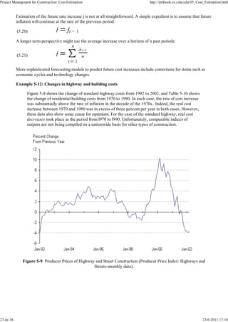
example, the following empirical model was estimated for maintenance expenditures on sections of the Ohio
Turnpike:
C = 596 + 0.0019 V + 21.7 A
where C is the annual cost of routine maintenance per lane-mile (in 1967 dollars), V is the volume of traffic on
the roadway (measured in equivalent standard axle loads, ESAL, so that a heavy truck is represented as
33 de 38 23/6/2011 17:10](https://image.slidesharecdn.com/5-costestimation-110716160453-phpapp01/85/5-cost-estimation-33-320.jpg)
![Project Management for Construction: Cost Estimation http://pmbook.ce.cmu.edu/05_Cost_Estimation.html
equivalent to many automobiles), and A is the age of the pavement in years since the last resurfacing.
According to this model, routine maintenance costs will increase each year as the pavement service
deteriorates. In addition, maintenance costs increase with additional pavement stress due to increased traffic
or to heavier axle loads, as reflected in the variable V.
For example, for V = 500,300 ESAL and A = 5 years, the annual cost of routine maintenance per lane-mile is
estimated to be:
C = 596 + (0.0019)(500,300) + (21.7)(5)
= 596 + 950.5 + 108.5 = 1,655 (in 1967 dollars)
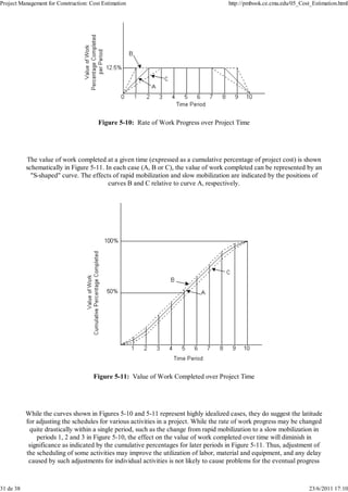
Example 5-18: Time stream of costs over the life of a roadway [7]
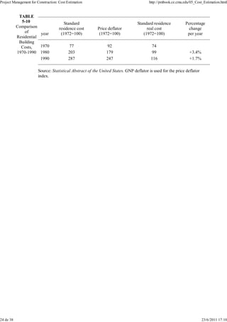
The time stream of costs over the life of a roadway depends upon the intervals at which rehabilitation is
carried out. If the rehabilitation strategy and the traffic are known, the time stream of costs can be estimated.
Using a life cycle model which predicts the economic life of highway pavement on the basis of the effects of
traffic and other factors, an optimal schedule for rehabilitation can be developed. For example, a time stream
of costs and resurfacing projects for one pavement section is shown in Figure 5-11. As described in the
previous example, the routine maintenance costs increase as the pavement ages, but decline after each new
resurfacing. As the pavement continues to age, resurfacing becomes more frequent until the roadway is
completely reconstructed at the end of 35 years.
Figure 5-11: Time Stream of Costs over the Life of a Highway Pavement
Back to top
5.14 References
1. Ahuja, H.N. and W.J. Campbell, Estimating: From Concept to Completion, Prentice-Hall, Inc.,
Englewood Cliffs, NJ, 1987.
2. Clark, F.D., and A.B. Lorenzoni, Applied Cost Engineering, Marcel Dekker, Inc., New York, 1978.
3. Clark, J.E., Structural Concrete Cost Estimating, McGraw-Hill, Inc., New York, 1983.
4. Diekmann, J.R., "Probabilistic Estimating: Mathematics and Applications," ASCE Journal of
34 de 38 23/6/2011 17:10](https://image.slidesharecdn.com/5-costestimation-110716160453-phpapp01/85/5-cost-estimation-34-320.jpg)

The document discusses cost estimation for construction projects. It describes the major categories of costs for a construction project, which include initial capital costs like construction, land acquisition, and design fees, as well as ongoing operation and maintenance costs. It also discusses approaches to cost estimation, including estimating based on historical cost data, unit costs, and computer-aided methods. Cost contingencies are also addressed.


![Eva[1]](https://cdn.slidesharecdn.com/ss_thumbnails/eva1-110703082755-phpapp01-thumbnail.jpg?width=640&height=640&fit=bounds)


