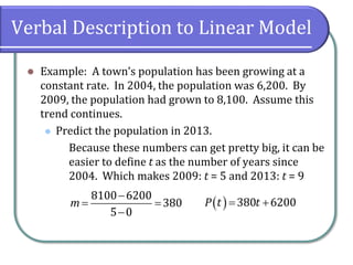
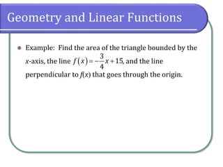
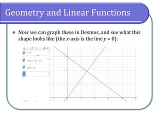
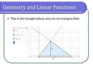
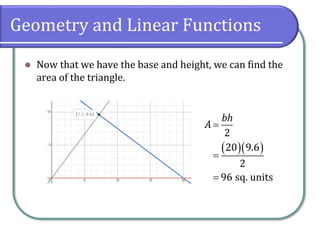
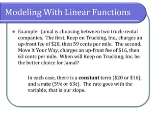
4.2 Modeling With Linear
Functions
Chapter 4 Linear Functions
Concepts & Objectives
⚫ Objectives for this section are
⚫ Build linear models from verbal descriptions.
⚫ Model a set of data with a linear function.
Verbal Description to Linear Model
⚫ When building linear models to solve problems
involving quantities with a constant rate of change, we
typically follow the same problem strategies that we
would use for any type of function.
⚫ In these problems, we will either be given the rate of
change (i.e. the slope) or at least two points to use to
calculate the slope.
⚫ Plug this information into the point-slope form of a line
and simplify to arrive at your function.
( ) ( ) ( )
1 1 1 1
y y m x x f x m x x y
− = −  = − +
Verbal Description to Linear Model
⚫ Example: A town’s population has been growing at a
constant rate. In 2004, the population was 6,200. By
2009, the population had grown to 8,100. Assume this
trend continues.
⚫ Predict the population in 2013.
Verbal Description to Linear Model
⚫ Example: A town’s population has been growing at a
constant rate. In 2004, the population was 6,200. By
2009, the population had grown to 8,100. Assume this
trend continues.
⚫ Predict the population in 2013.
First, we have to create a function. We have two
points of data: (2004, 6200) and (2009, 8100).
From this we can calculate the slope:
8100 6200 1900
380
2009 2004 5
m
−
= = =
−
Verbal Description to Linear Model
⚫ Example: A town’s population has been growing at a
constant rate. In 2004, the population was 6,200. By
2009, the population had grown to 8,100. Assume this
trend continues.
⚫ Predict the population in 2013.
Now we can plug in one of our data points to
create the function:
( ) ( )
380 2009 8100
380 755320
P t t
t
= − +
= −
Verbal Description to Linear Model
⚫ Example: A town’s population has been growing at a
constant rate. In 2004, the population was 6,200. By
2009, the population had grown to 8,100. Assume this
trend continues.
⚫ Predict the population in 2013.
Plug in 2013 for t to get the population:
( ) ( )
2013 380 2013 755320
9,620 in 2013
P = −
=
Verbal Description to Linear Model
⚫ Example: A town’s population has been growing at a
constant rate. In 2004, the population was 6,200. By
2009, the population had grown to 8,100. Assume this
trend continues.
⚫ Predict the population in 2013.
Because these numbers can get pretty big, it can be
easier to define t as the number of years since
2004. Which makes 2009: t = 5 and 2013: t = 9
8100 6200
380
5 0
m
−
= =
−
( ) 380 6200
P t t
= +
Verbal Description to Linear Model
⚫ Example: A town’s population has been growing at a
constant rate. In 2004, the population was 6,200. By
2009, the population had grown to 8,100. Assume this
trend continues.
⚫ Predict the population in 2013.
This makes our problem:
( ) ( )
9 380 9 6200
9,620 in 2013
P = +
=
Verbal Description to Linear Model
⚫ Example: A town’s population has been growing at a
constant rate. In 2004, the population was 6,200. By
2009, the population had grown to 8,100. Assume this
trend continues.
⚫ When will the population reach 15,000?
Using the previous definition of t, we can set the
function equal to 15,000 and solve t.
380 6200 15000
380 8800
23.16 years after 2004
or 2027
t
t
t
+ =
=

Geometry and Linear Functions
⚫ Since linear functions create graphs of lines,
intersections of collections of linear functions can create
geometric shapes.
⚫ If you are asked to find the area created by some linear
functions:
⚫ Graph the functions (using Desmos is easiest)
⚫ Triangle and parallelogram area formulas require
that you find the height and the base of the shape.
⚫ These are not always going to be vertical and
horizontal, but they must be perpendicular to each
other.
Geometry and Linear Functions
⚫ Example: Find the area of the triangle bounded by the
x-axis, the line , and the line
perpendicular to f(x) that goes through the origin.
( )
3
15
4
f x x
= − +
Geometry and Linear Functions
⚫ Example: Find the area of the triangle bounded by the
x-axis, the line , and the line
perpendicular to f(x) that goes through the origin.
First, we have to find the third line, which we’ll call
g(x). Recall that the perpendicular slope is the
negative reciprocal of the other slope:
( )
3
15
4
f x x
= − +
( ) ( ) ( )
4 4
0 0
3 3
g x x g x x
= − +  =
Geometry and Linear Functions
⚫ Now we can graph these in Desmos, and see what this
shape looks like (the x-axis is the line y = 0):
Geometry and Linear Functions
⚫ This is the triangle whose area we are trying to find:
h
b
Geometry and Linear Functions
⚫ We can see that the base is 20 units, but the height is a
little trickier. We need the y-coordinate of the
intersection.
⚫ There are two ways to find the intersection point
⚫ Set the two functions equal to each other and solve
for x and find y.
Geometry and Linear Functions
⚫ There are two ways to find the intersection point
⚫ Set the two functions equal to each other and solve
for x and find y.
4 3
15
3 4
3 4
15
4 3
25
15
12
12 36
15 7.2
25 5
x x
x x
x
x
= − +
+ =
=
 
= = =
 
 
( )
4
7.2 9.6
3
y = =
Geometry and Linear Functions
⚫ There are two ways to find the intersection point
⚫ Click on the intersection in Desmos:
⚫ So, the height of the triangle is 9.6 units.
(Obviously, the Desmos
method is easier, but
sometimes you might
need a fraction as an
answer, which Desmos
does not provide.)
Geometry and Linear Functions
⚫ Now that we have the base and height, we can find the
area of the triangle.
( )( )
2
20 9.6
2
96 sq. units
bh
A =
=
=
Modeling With Linear Functions
⚫ Real-world situations including two or more linear
functions may be modeled with a system of linear
equations.
⚫ Find the solution by setting two linear functions equal to
each other and solving for x, or find the point of
intersection on a graph.
Modeling With Linear Functions
⚫ Example: Jamal is choosing between two truck-rental
companies. The first, Keep on Trucking, Inc., charges an
up-front fee of $20, then 59 cents per mile. The second,
Move It Your Way, charges an up-front fee of $16, then
63 cents per mile. When will Keep on Trucking, Inc. be
the better choice for Jamal?
In each case, there is a constant term ($20 or $16),
and a rate (59¢ or 63¢). The rate goes with the
variable; that is our slope.
Modeling With Linear Functions
⚫ Example: Jamal is choosing between two truck-rental
companies. The first, Keep on Trucking, Inc., charges an
up-front fee of $20, then 59 cents per mile. The second,
Move It Your Way, charges an up-front fee of $16, then
63 cents per mile. When will Keep on Trucking, Inc. be
the better choice for Jamal?
Driving 0 miles gives us the y-intercept:
( )
( )
0.59 20
0.63 16
K d d
M d d
= +
= +
Modeling With Linear Functions
⚫ Example: Jamal is choosing between two truck-rental
companies. The first, Keep on Trucking, Inc., charges an
up-front fee of $20, then 59 cents per mile. The second,
Move It Your Way, charges an up-front fee of $16, then
63 cents per mile. When will Keep on Trucking, Inc. be
the better choice for Jamal?
Keep on Trucking will be the better choice when
( ) ( ) or
K d M d
 0.59 20 0.63 16
0.04 4
100 miles
d d
d
d
+  +
−  −

Modeling With Linear Functions
⚫ Once you have your functions set up, you can also graph
the functions and find the intersection point:
Classwork
⚫ College Algebra 2e
⚫ 4.2: 6,8,12-15 (all); 4.1: 40-68 (×4); 3.7: 38-46 (even)
⚫ 4.2 Classwork Check
⚫ Quiz 4.1

4.2 Modeling With Linear Functions

  • 1.
    4.2 Modeling WithLinear Functions Chapter 4 Linear Functions
  • 2.
    Concepts & Objectives ⚫Objectives for this section are ⚫ Build linear models from verbal descriptions. ⚫ Model a set of data with a linear function.
  • 3.
    Verbal Description toLinear Model ⚫ When building linear models to solve problems involving quantities with a constant rate of change, we typically follow the same problem strategies that we would use for any type of function. ⚫ In these problems, we will either be given the rate of change (i.e. the slope) or at least two points to use to calculate the slope. ⚫ Plug this information into the point-slope form of a line and simplify to arrive at your function. ( ) ( ) ( ) 1 1 1 1 y y m x x f x m x x y − = −  = − +
  • 4.
    Verbal Description toLinear Model ⚫ Example: A town’s population has been growing at a constant rate. In 2004, the population was 6,200. By 2009, the population had grown to 8,100. Assume this trend continues. ⚫ Predict the population in 2013.
  • 5.
    Verbal Description toLinear Model ⚫ Example: A town’s population has been growing at a constant rate. In 2004, the population was 6,200. By 2009, the population had grown to 8,100. Assume this trend continues. ⚫ Predict the population in 2013. First, we have to create a function. We have two points of data: (2004, 6200) and (2009, 8100). From this we can calculate the slope: 8100 6200 1900 380 2009 2004 5 m − = = = −
  • 6.
    Verbal Description toLinear Model ⚫ Example: A town’s population has been growing at a constant rate. In 2004, the population was 6,200. By 2009, the population had grown to 8,100. Assume this trend continues. ⚫ Predict the population in 2013. Now we can plug in one of our data points to create the function: ( ) ( ) 380 2009 8100 380 755320 P t t t = − + = −
  • 7.
    Verbal Description toLinear Model ⚫ Example: A town’s population has been growing at a constant rate. In 2004, the population was 6,200. By 2009, the population had grown to 8,100. Assume this trend continues. ⚫ Predict the population in 2013. Plug in 2013 for t to get the population: ( ) ( ) 2013 380 2013 755320 9,620 in 2013 P = − =
  • 8.
    Verbal Description toLinear Model ⚫ Example: A town’s population has been growing at a constant rate. In 2004, the population was 6,200. By 2009, the population had grown to 8,100. Assume this trend continues. ⚫ Predict the population in 2013. Because these numbers can get pretty big, it can be easier to define t as the number of years since 2004. Which makes 2009: t = 5 and 2013: t = 9 8100 6200 380 5 0 m − = = − ( ) 380 6200 P t t = +
  • 9.
    Verbal Description toLinear Model ⚫ Example: A town’s population has been growing at a constant rate. In 2004, the population was 6,200. By 2009, the population had grown to 8,100. Assume this trend continues. ⚫ Predict the population in 2013. This makes our problem: ( ) ( ) 9 380 9 6200 9,620 in 2013 P = + =
  • 10.
    Verbal Description toLinear Model ⚫ Example: A town’s population has been growing at a constant rate. In 2004, the population was 6,200. By 2009, the population had grown to 8,100. Assume this trend continues. ⚫ When will the population reach 15,000? Using the previous definition of t, we can set the function equal to 15,000 and solve t. 380 6200 15000 380 8800 23.16 years after 2004 or 2027 t t t + = = 
  • 11.
    Geometry and LinearFunctions ⚫ Since linear functions create graphs of lines, intersections of collections of linear functions can create geometric shapes. ⚫ If you are asked to find the area created by some linear functions: ⚫ Graph the functions (using Desmos is easiest) ⚫ Triangle and parallelogram area formulas require that you find the height and the base of the shape. ⚫ These are not always going to be vertical and horizontal, but they must be perpendicular to each other.
  • 12.
    Geometry and LinearFunctions ⚫ Example: Find the area of the triangle bounded by the x-axis, the line , and the line perpendicular to f(x) that goes through the origin. ( ) 3 15 4 f x x = − +
  • 13.
    Geometry and LinearFunctions ⚫ Example: Find the area of the triangle bounded by the x-axis, the line , and the line perpendicular to f(x) that goes through the origin. First, we have to find the third line, which we’ll call g(x). Recall that the perpendicular slope is the negative reciprocal of the other slope: ( ) 3 15 4 f x x = − + ( ) ( ) ( ) 4 4 0 0 3 3 g x x g x x = − +  =
  • 14.
    Geometry and LinearFunctions ⚫ Now we can graph these in Desmos, and see what this shape looks like (the x-axis is the line y = 0):
  • 15.
    Geometry and LinearFunctions ⚫ This is the triangle whose area we are trying to find: h b
  • 16.
    Geometry and LinearFunctions ⚫ We can see that the base is 20 units, but the height is a little trickier. We need the y-coordinate of the intersection. ⚫ There are two ways to find the intersection point ⚫ Set the two functions equal to each other and solve for x and find y.
  • 17.
    Geometry and LinearFunctions ⚫ There are two ways to find the intersection point ⚫ Set the two functions equal to each other and solve for x and find y. 4 3 15 3 4 3 4 15 4 3 25 15 12 12 36 15 7.2 25 5 x x x x x x = − + + = =   = = =     ( ) 4 7.2 9.6 3 y = =
  • 18.
    Geometry and LinearFunctions ⚫ There are two ways to find the intersection point ⚫ Click on the intersection in Desmos: ⚫ So, the height of the triangle is 9.6 units. (Obviously, the Desmos method is easier, but sometimes you might need a fraction as an answer, which Desmos does not provide.)
  • 19.
    Geometry and LinearFunctions ⚫ Now that we have the base and height, we can find the area of the triangle. ( )( ) 2 20 9.6 2 96 sq. units bh A = = =
  • 20.
    Modeling With LinearFunctions ⚫ Real-world situations including two or more linear functions may be modeled with a system of linear equations. ⚫ Find the solution by setting two linear functions equal to each other and solving for x, or find the point of intersection on a graph.
  • 21.
    Modeling With LinearFunctions ⚫ Example: Jamal is choosing between two truck-rental companies. The first, Keep on Trucking, Inc., charges an up-front fee of $20, then 59 cents per mile. The second, Move It Your Way, charges an up-front fee of $16, then 63 cents per mile. When will Keep on Trucking, Inc. be the better choice for Jamal?
  • 22.
    Modeling With LinearFunctions ⚫ Example: Jamal is choosing between two truck-rental companies. The first, Keep on Trucking, Inc., charges an up-front fee of $20, then 59 cents per mile. The second, Move It Your Way, charges an up-front fee of $16, then 63 cents per mile. When will Keep on Trucking, Inc. be the better choice for Jamal? In each case, there is a constant term ($20 or $16), and a rate (59¢ or 63¢). The rate goes with the variable; that is our slope.
  • 23.
    Modeling With LinearFunctions ⚫ Example: Jamal is choosing between two truck-rental companies. The first, Keep on Trucking, Inc., charges an up-front fee of $20, then 59 cents per mile. The second, Move It Your Way, charges an up-front fee of $16, then 63 cents per mile. When will Keep on Trucking, Inc. be the better choice for Jamal?
  • 24.
    Modeling With LinearFunctions ⚫ Example: Jamal is choosing between two truck-rental companies. The first, Keep on Trucking, Inc., charges an up-front fee of $20, then 59 cents per mile. The second, Move It Your Way, charges an up-front fee of $16, then 63 cents per mile. When will Keep on Trucking, Inc. be the better choice for Jamal? Driving 0 miles gives us the y-intercept: ( ) ( ) 0.59 20 0.63 16 K d d M d d = + = +
  • 25.
    Modeling With LinearFunctions ⚫ Example: Jamal is choosing between two truck-rental companies. The first, Keep on Trucking, Inc., charges an up-front fee of $20, then 59 cents per mile. The second, Move It Your Way, charges an up-front fee of $16, then 63 cents per mile. When will Keep on Trucking, Inc. be the better choice for Jamal? Keep on Trucking will be the better choice when ( ) ( ) or K d M d  0.59 20 0.63 16 0.04 4 100 miles d d d d +  + −  − 
  • 26.
    Modeling With LinearFunctions ⚫ Once you have your functions set up, you can also graph the functions and find the intersection point:
  • 27.
    Classwork ⚫ College Algebra2e ⚫ 4.2: 6,8,12-15 (all); 4.1: 40-68 (×4); 3.7: 38-46 (even) ⚫ 4.2 Classwork Check ⚫ Quiz 4.1