Causality models

UNIVERSITY OF ECONOMICS, HO CHI MINH CITY
FACULTY OF DEVELOPMENT ECONOMICS

TIME SERIES ECONOMETRICS
CAUSALITY MODELS
Compiled by Phung Thanh Binh1 (2010)

“You could not step twice into the same river; for other waters are ever
flowing on to you.” Heraclitus (540 – 380 BC)

The aim of this lecture is to provide you with the key
concepts of time series econometrics. To its end, you
are able to understand time series based researches,
officially published in international journals2 such
as applied economics, applied econometrics, and the
likes. Moreover, I also expect that some of you will
be interested in time series data analysis, and choose
the related topics for your future thesis. As the time
this lecture is compiled, I believe that the Vietnam

1
Faculty of Development Economics, University of Economics, HCMC. Email: ptbinh@ueh.edu.vn.
2
Selected papers were compiled by Phung Thanh Binh & Vo Duc Hoang Vu (2009). You can find them
at the H library.

1

time series data3 is long enough for you to conduct
such studies.

Specifically, this lecture will provide you the
following points:

An overview of time series econometrics

Stationary versus non-stationary

Unit roots and spurious regressions

Testing for unit roots

Vector autoregressive models

Causality tests

Cointegration and error correction models

Optimal lag length selection criteria

Basic practicalities in using Eviews 6.0

Suggested research topics

1. AN OVERVIEW OF TIME SERIES ECONOMETRICS

In this lecture, we will mainly discuss single
equation estimation techniques in a very different way
from what you have previously learned in the basic
econometrics course. According to Asteriou (2007),
there are various aspects to time series analysis but
the most common theme to them is to fully exploit the
dynamic structure in the data. Saying differently, we
will extract as much information as possible from the

3
The most important data sources for these studies can be World Bank’s World Development Indicators,
IMF-IFS, GSO, and Reuters Thomson.

2

past history of the series. The analysis of time
series is usually explored within two fundamental
types, namely time series forecasting4 and dynamic
modelling. Pure time series forecasting, such as ARIMA
models5, is often mentioned as univariate analysis.
Unlike most other econometrics, in univariate analysis
we do not concern much with building structural
models, understanding the economy or testing
hypothesis6, but what we really concern is developing
efficient models, which are able to forecast well. The
efficient forecasting models can be evaluated using
various criteria such as AIC, SBC7, RMSE, correlogram,
and fitted-actual value comparison8. In these cases,
we try to exploit the dynamic inter-relationship,
which exists over time for any single variable (say,
sales, GDP, stock prices, ect). On the other hand,
dynamic modelling, including bivariate and
multivariate time series analysis, is still concerned
with understanding the structure of the economy and
testing hypothesis. However, this kind of modelling is
based on the view that most economic series are slow
to adjust to any shock and so to understand the
process must fully capture the adjustment process
which may be long and complex (Asteriou, 2007). The
dynamic modelling has become increasingly popular
thanks to the works of two Nobel laureates, namely,

4
See Nguyen Trong Hoai et al, 2009.
5
You already learned this topic from Dr Cao Hao Thi.
6
Both statistical hypothesis and economic hypothesis.
7
SBC and SIC are interchangeably used in econometrics books and empirical studies.
8

3

Clive W.J. Granger (for methods of analyzing economic
time series with common trends, or cointegration) and
Robert F. Engle (for methods of analyzing economic
time series with time-varying volatility or ARCH)9. Up
to now, dynamic modelling has remarkably contributed
to economic policy formulation in various fields.
Generally, the key purpose of time series analysis is
to capture and examine the dynamics of the data.

In time series econometrics, it is equally important
that the analysts should clearly understand the term
“stochastic process”. According to Gujarati (2003)10, a
random or stochastic process is a collection of random
variables ordered in time. If we let Y denote a random
variable, and if it is continuous, we denote it a
Y(t), but if it is discrete, we denote it as Yt. Since
most economic data are collected at discrete points in
time, we usually use the notation Yt rather than Y(t).
If we let Y represent GDP, we have Y1, Y2, Y3, …, Y88,
where the subscript 1 denotes the first observation
(i.e., GDP for the first quarter of 1970) and the
subscript 88 denotes the last observation (i.e., GDP
for the fourth quarter of 1991). Keep in mind that
each of these Y’s is a random variable.

In what sense we can regard GDP as a stochastic
process? Consider for instance the GDP of $2872.8
billion for 1970Q1. In theory, the GDP figure for the
first quarter of 1970 could have been any number,
depending on the economic and political climate then

9
http://nobelprize.org/nobel_prizes/economics/laureates/2003/
10
Note that I completely cite this from Gujarati (2003).

4

prevailing. The figure of $2872.8 billion is just a
particular realization of all such possibilities. In
this case, we can think of the value of $2872.8
billion as the mean value of all possible values of
GDP for the first quarter of 1970. Therefore, we can
say that GDP is a stochastic process and the actual
values we observed for the period 1970Q1 to 1991Q4 are
a particular realization of that process. Gujarati
(2003) states that the distinction between the
stochastic process and its realization in time series
data is just like the distinction between population
and sample in cross-sectional data. Just as we use
sample data to draw inferences about a population; in
time series, we use the realization to draw inferences
about the underlying stochastic process.

The reason why I mention this term before examining
specific models is that all basic assumptions in time
series models relate to the stochastic process
(population). Stock & Watson (2007) say that the
assumption that the future will be like the past is an
important one in time series regression. If the future
is like the past, then the historical relationships
can be used to forecast the future. But if the future
differs fundamentally from the past, then the
historical relationships might not be reliable guides
to the future. Therefore, in the context of time
series regression, the idea that historical
relationships can be generalized to the future is
formalized by the concept of stationarity.

5

2. STATIONARY STOCHASTIC PROCESSES

2.1 Definition

According to Gujarati (2003), a key concept underlying
stochastic process that has received a great deal of
attention and scrutiny by time series analysts is the
so-called stationary stochastic process. Broadly
speaking, a stochastic process is said to be
stationary if its mean and variance are constant over
time and the value of the covariance between the two
periods depends only on the distance or gap or lag
between the two time periods and not the actual time
at which the covariance is computed. In the time
series literature, such a stochastic process is known
as a weakly stationary, or covariance stationary, or
second-order stationary, or wide sense, stochastic
process. By contrast, a time series is strictly
stationary if all the moments of its probability
distribution and not just the first two (i.e., mean
and variance) are invariant over time. If, however,
the stationary process is normal, the weakly
stationary stochastic process is also strictly
stationary, for the normal stochastic process is fully
specified by its two moments, the mean and the
variance. For most practical situations, the weak type
of stationarity often suffices. According to Asteriou
(2007), a time series is weakly stationary when it has
the following characteristics:

(a) exhibits mean reversion in that it fluctuates
around a constant long-run mean;

6

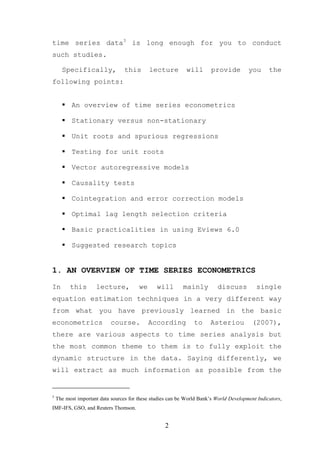
(b) has a finite variance that is time-invariant;
and

(c) has a theoretical correlogram that diminishes
as the lag length increases.

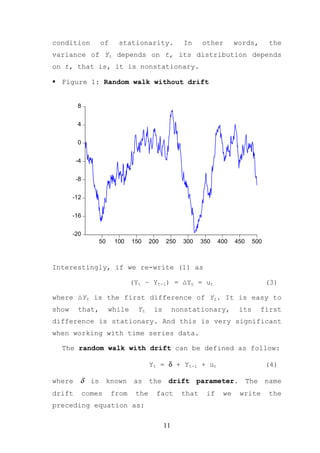
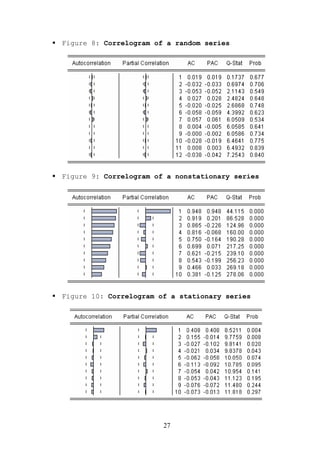
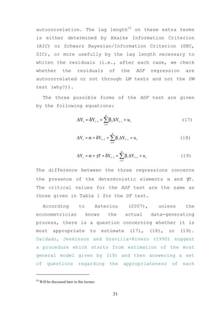
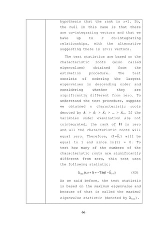
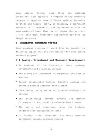
In its simplest terms a time series Yt is said to be
weakly stationary (hereafter refer to stationary) if:

(a) Mean: E(Yt) = µ (constant for all t);

(b) Variance: Var(Yt) = E(Yt-µ)2 = σ2 (constant for
all t); and

(c) Covariance: Cov(Yt,Yt+k) = γk = E[(Yt-µ)(Yt+k-µ)]

where γk, covariance (or autocovariance) at lag k,is
the covariance between the values of Yt and Yt+k, that
is, between two Y values k periods apart. If k = 0, we
obtain γ0, which is simply the variance of Y (=σ2); if
k = 1, γ1 is the covariance between two adjacent values
of Y.

Suppose we shift the origin of Y from Yt to Yt+m
(say, from the first quarter of 1970 to the first
quarter of 1975 for our GDP data). Now, if Yt is to be
stationary, the mean, variance, and autocovariance of
Yt+m must be the same as those of Yt. In short, if a
time series is stationary, its mean, variance, and
autocovariance (at various lags) remain the same no
matter at what point we measure them; that is, they
are time invariant. According to Gujarati (2003), such
time series will tend to return to its mean (called
mean reversion) and fluctuations around this mean
(measured by its variance) will have a broadly
constant amplitude.

7

If a time series is not stationary in the sense just
defined, it is called a nonstationary time series. In
other words, a nonstationary time series will have a
time-varying mean or a time-varying variance or both.

Why are stationary time series so important?
According to Gujarati (2003), because if a time series
is nonstationary, we can study its behavior only for
the time period under consideration. Each set of time
series data will therefore be for a particular
episode. As a consequence, it is not possible to
generalize it to other time periods. Therefore, for
the purpose of forecasting or policy analysis, such
(nonstationary) time series may be of little practical
value. Saying differently, stationarity is important
because if the series is nonstationary, then all the
typical results of the classical regression analysis
are not valid. Regressions with nonstationary time
series may have no meaning and are therefore called
“spurious” (Asteriou, 2007).

In addition, a special type of stochastic process
(or time series), namely, a purely random, or white
noise, process, is also popular in time series
econometrics. According to Gujarati (2003), we call a
stochastic process purely random if it has zero mean,
constant variance σ2, and is serially uncorrelated.
This is similar to what we call the error term, ut, in
the classical normal linear regression model, once
discussed in the phenomenon of serial correlation
topic. This error term is often denoted as ut ~
iid(0,σ2).

8

2.2 Random Walk Process

According to Stock and Watson (2007), time series
variables can fail to be stationary in various ways,
but two are especially relevant for regression
analysis of economic time series data: (1) the series
can have persistent, long-run movements, that is, the
series can have trends; and, (2) the population
regression can be unstable over time, that is, the
population regression can have breaks. For the purpose
of this lecture, I only focus on the first type of
nonstationarity.

A trend is a persistent long-term movement of a
variable over time. A time series variable fluctuates
around its trend. There are two types of trends seen
in time series data: deterministic and stochastic. A
deterministic trend is a nonrandom function of time
(i.e., Yt = a + b*Time, Yt = a + b*Time + c*Time2, and
so on). In contrast, a stochastic trend is random and
varies over time. According to Stock and Watson
(2007), it is more appropriate to model economic time
series as having stochastic rather than deterministic
trends. Therefore, our treatment of trends in economic
time series focuses on stochastic rather than
deterministic trends, and when we refer to “trends” in
time series data, we mean stochastic trends unless we
explicitly say otherwise.

The simplest model of a variable with a stochastic
trend is the random walk. There are two types of
random walks: (1) random walk without drift (i.e., no

9

constant or intercept term) and (2) random walk with
drift (i.e., a constant term is present).

The random walk without drift is defined as follow.
Suppose ut is a white noise error term with mean 0 and
variance σ2. The Yt is said to be a random walk if:

Yt = Yt-1 + ut (1)

The basic idea of a random walk is that the value of
the series tomorrow is its value today, plus an
unpredictable change.

From (1), we can write

Y1 = Y0 + u1

Y2 = Y1 + u2 = Y0 + u1 + u2

Y3 = Y2 + u3 = Y0 + u1 + u2 + u3

Y4 = Y3 + u4 = Y0 + u1 + … + u4

…

Yt = Yt-1 + ut = Y0 + u1 + … + ut

In general, if the process started at some time 0 with
a value Y0, we have

Yt = Y0 + ∑ u t (2)

therefore,

E(Yt ) = E(Y0 + ∑ u t ) = Y0

In like fashion, it can be shown that

Var (Yt ) = E(Y0 + ∑ u t − Y0 ) 2 = E(∑ u t ) 2 = tσ 2

Therefore, the mean of Y is equal to its initial or
starting value, which is constant, but as t increases,
its variance increases indefinitely, thus violating a

10

condition of stationarity. In other words, the
variance of Yt depends on t, its distribution depends
on t, that is, it is nonstationary.

Figure 1: Random walk without drift

8

4

0

-4

-8

-12

-16

-20
50 100 150 200 250 300 350 400 450 500

Interestingly, if we re-write (1) as

(Yt – Yt-1) = ∆Yt = ut (3)

where ∆Yt is the first difference of Yt. It is easy to
show that, while Yt is nonstationary, its first
difference is stationary. And this is very significant
when working with time series data.

The random walk with drift can be defined as follow:

Yt = δ + Yt-1 + ut (4)

where δ is known as the drift parameter. The name
drift comes from the fact that if we write the
preceding equation as:

11

Yt – Yt-1 = ∆Yt = δ + ut (5)

it shows that Yt drifts upward or downward, depending
on δ being positive or negative. We can easily show
that, the random walk with drift violates both
conditions of stationarity:

E(Yt) = Y0 + t.δ

Var(Yt) = tσ2

In other words, both mean and variance of Yt depends
on t, its distribution depends on t, that is, it is
nonstationary.

Figure 2: Random walk with drift

30

25

20

15

10

5

0

-5

-10
50 100 150 200 250 300 350 400 450 500

Yt = 2 + Yt-1 + ut

12

Figure 3: Random walk with drift

10

5

0

-5

-10

-15

-20

-25
50 100 150 200 250 300 350 400 450 500

Yt = -2 + Yt-1 + ut

Stock and Watson (2007) say that because the variance
of a random walk increases without bound, its
population autocorrelations are not defined (the first
autocovariance and variance are infinite and the ratio
of the two is not well defined)11.

2.3 Unit Root Stochastic Process

According to Gujarati (2003), the random walk model is
an example of what is known in the literature as a
unit root process.

11
Cov(Yt , Yt −1 ) ∞
Corr(Yt,Yt-1) = ~
Var (Yt )Var (Yt −1 ) ∞

13

Let us write the random walk model (1) as:

Yt = ρYt-1 + ut (-1 ≤ ρ ≤ 1) (6)

This model resembles the Markov first-order
autoregressive model, mentioned in the basic
econometrics course, autocorrelation topic. If ρ = 1,
(6) becomes a random walk without drift. If ρ is in
fact 1, we face what is known as the unit root
problem, that is, a situation of nonstationarity. The
name unit root is due to the fact that ρ = 1.
Technically, if ρ = 1, we can write (6) as Yt – Yt-1 =
ut. Now using the lag operator L so that Lyt = Yt-1, L2Yt
= Yt-2, and so on, we can write (6) as (1-L)Yt = ut. If
we set (1-L) = 0, we obtain, L = 1, hence the name
unit root. Thus, the terms nonstationarity, random
walk, and unit root can be treated as synonymous.

If, however, ρ ≤ 1, that is if the absolute value

of ρ is less than one, then it can be shown that the
time series Yt is stationary.

2.4 Illustrative Examples

Consider the AR(1) model as presented in equation (6).
Generally, we can have three possible cases:

Case 1: ρ < 1 and therefore the series Yt is
stationary. A graph of a stationary series
for ρ = 0.67 is presented in Figure 4.

Case 2: ρ > 1 where in this case the series
explodes. A graph of an explosive series for
ρ = 1.26 is presented in Figure 5.

14

Case 3: ρ = 1 where in this case the series contains
a unit root and is non-stationary. Graph of
stationary series for ρ = 1 are presented in
Figure 6.

In order to reproduce the graphs and the series which
are stationary, exploding and nonstationary, we type
the following commands in Eviews:

Step 1: Open a new workfile (say, undated type),
containing 200 observations.

Step 2: Generate X, Y, Z as the following commands:

smpl 1 1

genr X=0

genr Y=0

genr Z=0

smpl 2 200

genr X=0.67*X(-1)+nrnd

genr Y=1.26*Y(-1)+nrnd

genr Z=Z(-1)+nrnd

smpl 1 200

Step 3: Plot X, Y, Z using the line plot type (Figure
4, 5, and 6).

plot X

plot Y

plot Z

15

Figure 4: Stationary series

5

4

3

2

1

0

-1

-2

-3

-4
25 50 75 100 125 150 175 200

Figure 5: Explosive series

1.6E+19

1.4E+19

1.2E+19

1.0E+19

8.0E+18

6.0E+18

4.0E+18

2.0E+18

0.0E+00
25 50 75 100 125 150 175 200

16

Figure 6: Nonstationary series

5

0

-5

-10

-15

-20

-25
25 50 75 100 125 150 175 200

3. UNIT ROOTS AND SPURIOUS REGRESSIONS

3.1 Spurious Regressions

Most macroeconomic time series are trended and
therefore in most cases are nonstationary (see for
examples time plots of imports, exports, money supply,
FDI, GDP, CPI, market interest rates, and so on for
the Vietnam economy12). The problem with nonstationary
or trended data is that the standard ordinary least
squares (OLS) regression procedures can easily lead to
incorrect conclusions. According to Asteriou (2007),
it can be shown in these cases that the regression
results have very high value of R2 (sometimes even
higher than 0.95) and very high values of t-ratios

12
These data are now available at the H library.

17

(sometimes even higher than 4), while the variables
used in the analysis have no real interrelationships.

Asteriou (2007) states that many economic series
typically have an underlying rate of growth, which may
or may not be constant, for example GDP, prices or
money supply all tend to grow at a regular annual
rate. Such series are not stationary as the mean is
continually rising however they are also not
integrated as no amount of differencing can make them
stationary. This gives rise to one of the main reasons
for taking the logarithm of data before subjecting it
to formal econometric analysis. If we take the
logarithm of a series, which exhibits an average
growth rate we will turn it into a series which
follows a linear trend and which is integrated. This
can be easily seen formally. Suppose we have a series
Xt, which increases by 10% every period, thus:

Xt = 1.1Xt-1

If we then take the logarithm of this we get

log(Xt) = log(1.1) + log(Xt-1)

Now the lagged dependent variable has a unit
coefficient and each period it increases by an
absolute amount equal to log(1.1), which is of course
constant. This series would now be I(1)13.

More formally, consider the model:

Yt = β1 + β2Xt + ut (7)

13
See Gujarati (2003: 804-806)

18

where ut is the error term. The assumptions of
classical linear regression model (CLRM) require both
Yt and Xt to have zero and constant variance (i.e., to
be stationary). In the presence of nonstationarity,
then the results obtained from a regression of this
kind are totally spurious14 and these regressions are
called spurious regressions.

The intuition behind this is quite simple. Over
time, we expect any nonstationary series to wander
around (see Figure 7), so over any reasonably long
sample the series either drift up or down. If we then
consider two completely unrelated series which are
both nonstationary, we would expect that either they
will both go up or down together, or one will go up
while the other goes down. If we then performed a
regression of one series on the other, we would then
find either a significant positive relationship if
they are going in the same direction or a significant
negative one if they are going in opposite directions
even though really they are both unrelated. This is
the essence of a spurious regression.

It is said that a spurious regression usually has a
very high R2 , t statistics that appear to provide
significant estimates, but the results may have no
economic meaning. This is because the OLS estimates
may not be consistent, and therefore the tests of
statistical inference are not valid.

14
This was first introduced by Yule (1926), and re-examined by Granger and Newbold (1974) using the
Monte Carlo simulations.

19

Granger and Newbold (1974) constructed a Monte Carlo
analysis generating a large number of Yt and Xt series
containing unit roots following the formulas:

Yt = Yt-1 + eYt (8)

Xt = Xt-1 + eXt (9)

where eYt and eXt are artificially generated normal
random numbers.

Since Yt and Xt are independent of each other, any
regression between them should give insignificant
results. However, when they regressed the various Yts
to the Xts as show in equation (8), they surprisingly
found that they were unable to reject the null
hypothesis of β2 = 0 for approximately 75% of their
cases. They also found that their regressions had very
high R2s and very low values of DW statistics.

To see the spurious regression problem, we can type
the following commands in Eviews (after opening the
new workfile, say, undated with 500 observations) to
see how many times we can reject the null hypothesis
of β2 = 0. The commands are:

smpl @first @first+1 (or smpl 1 1)

genr Y=0

genr X=0

smpl @first+1 @last (or smpl 2 500)

genr Y=Y(-1)+nrnd

genr X=X(-1)+nrnd

scat(r) Y X

smpl @first @last

20

ls Y c X

An example of a scatter plot of Y against X obtained
in this way is shown in Figure 7. The estimated
equation is:

Figure 7: Scatter plot of a spurious regression

10

0

-10

-20
Y

-30

-40

-50
-10 -5 0 5 10 15 20 25

X

21

Granger and Newbold (1974) proposed the following
“rule of thumb” for detecting spurious regressions: If
R2 > DW statistic or if R2 ≈ 1 then the regression
‘must’ be spurious.

To understand the problem of spurious regression
better, it might be useful to use an example with real
economic data. This example was conducted by Asteriou
(2007). Consider a regression of the logarithm of real
GDP (Yt) to the logarithm of real money supply (Mt) and
a constant. The results obtained from such a
regression are the following:

Yt = 0.042 + 0.453Mt; R2 = 0.945; DW = 0.221

(4.743) (8.572)

Here we see very good t-ratios, with coefficients that
have the right signs and more or less plausible
magnitudes. The coefficient of determination is very
high (R2 = 0.945), but there is a high degree of
autocorrelation (DW = 0.221). This shows evidence of
the possible existence of spurious regression. In
fact, this regression is totally meaningless because
the money supply data are for the UK economy and the
GDP figures are for the US economy. Therefore,
although there should not be any significant
relationship, the regression seems to fit the data
very well, and this happens because the variables used
in the example are, simply, trended (nonstationary).
So, Asteriou (2007) recommends that econometricians
should be very careful when working with trended
variables.

22

3.2 Explaining the Spurious Regression Problem

According to Asteriou (2007), in a slightly more
formal way the source of the spurious regression
problem comes from the fact that if two variables, X
and Y, are both stationary, then in general any linear
combination of them will certainly be stationary. One
important linear combination of them is of course the
equation error, and so if both variables are
stationary, the error in the equation will also be
stationary and have a well-behaved distribution.
However, when the variables become nonstationary, then
of course we can not guarantee that the errors will be
stationary and in fact as a general rule (although not
always) the error itself be nonstationary and when
this happens, we violate the basic CLRM assumptions of
OLS regression. If the errors were nonstationary, we
would expect them to wander around and eventually get
large. But OLS regression because it selects the
parameters so as to make the sum of the squared errors
as small as possible will select any parameter which
gives the smallest error and so almost any parameter
value can result.

The simplest way to examine the behaviour of ut is
to rewrite (7) as:

ut = Yt – β1 – β2Xt (10)

or, excluding the constant β1 (which only affects ut
sequence by rescaling it):

ut = Yt – β2Xt (11)

23

If Yt and Xt are generated by equations (8) and (9),
then if we impose the initial conditions Y0 = X0 = 0 we
get that:

u t = Y0 + e Ý1 + e Ý 2 + ... + e Ýi + β 2 (X 0 + e X1 + e X 2 + ... + e Xi )

or
t t
u t = ∑ e Yi + β 2 ∑ e Xi (12)
i =1 i =1

From equation (12), we realize that the variance of
the error term will tend to become infinitely large as
t increases. Hence, the assumptions of the CLRM are
violated, and therefore, any t test, F test or R2 are
unreliable.

In terms of equation (7), there are four different
cases to discuss:

Case 1: Both Yt and Xt are stationary, and the CLRM is
appropriate with OLS estimates being BLUE.

Case 2: Yt and Xt are integrated of different orders15.
In this case, the regression equations are
meaningless.

Case 3: Yt and Xt are integrated of the same order and
the ut sequence contains a stochastic trend.
In this case, we have spurious regression and
it is often recommended to re-estimate the
regression equation in the first differences
or to re-specify it (usually by using the GLS
method, such as Orcutt-Cochrane procedure)16.

15
Denoted as I(d).
16

24

Case 4: Yt and Xt are integrated of the same order and
the ut is stationary. In this special case, Yt
and Xt are said to be cointegrated. This will
be examined in detail later.

4. TESTING FOR UNIT ROOTS

4.1 Graphical Analysis

According to Gujarati (2003), before one pursues
formal tests, it is always advisable to plot the time
series under study. Such a plot gives an initial clue
about the likely nature of the time series. Such a
intuitive feel is the starting point of formal tests
of stationary.

If you use Eviews to support your study, you can
easily instruct yourself by the Help function:
Help/Users Guide I (pdf)17.

4.2 Autocorrelation Function and Correlogram

Autocorrelation is the correlation between a variable
lagged one or more periods and itself. The correlogram
or autocorrelation function is a graph of the
autocorrelations for various lags of a time series
data. According to Hanke (2005), the autocorrelation
coefficients18 for different time lags for a variable
can be used to answer the following questions:

1. Are the data random? (This is usually used for
the diagnostic tests of forecasting models).

17
It is possible to read Nguyen Trong Hoai et al, 2009.
18
This is not shown in this lecture. You can make references from Gujarati (2003: 808-813), Hanke
(2005: 60-74), or Nguyen Trong Hoai et al (2009: Chapter 3, 4, and 8).

25

2. Do the data have a trend (nonstationary)?

3. Are the data stationary?

4. Are the data seasonal?

Besides, this is very useful when selecting the
appropriate p and q in the ARIMA models19.

If a series is random, the autocorrelations
between Yt and Yt-k for any lag k are close to
zero. The successive values of a time series are
not related to each other (Figure 8).

If a series has a trend, successive observations
are highly correlated, and the autocorrelation
coefficients are typically significantly different
from zero for the first several time lags and then
gradually drop toward zero as the number of lags
increases. The autocorrelation coefficient for
time lag 1 is often very large (close to 1). The
autocorrelation coefficient for time lag 2 will
also be large. However, it will not be as large as
for time lag 1 (Figure 9).

If a series is stationary, the autocorrelation
coefficients for lag 1 or lag 2 are significantly
different from zero and then suddenly die out as
the number of lags increases (Figure 10).

If a series has a seasonal pattern, a significant
autocorrelation coefficient will occur at the
seasonal time lag or multiples of seasonal lag
(Figure 11). This is not important within this
lecture context.

19

26

Figure 8: Correlogram of a random series

Figure 9: Correlogram of a nonstationary series

Figure 10: Correlogram of a stationary series

27

Figure 11: Correlogram of a seasonal series

The correlogram becomes very useful for time series
forecasting and other practical (business)
implications. If you conduct academic studies,
however, it is necessary to provide some formal
statistics such as t statistic, Box-Pierce Q
statistic, Ljung-Box (LB) statistic, or especially
unit root tests.

4.3 Simple Dickey-Fuller Test for Unit Roots

Dickey and Fuller (1979,1981) devised a procedure to
formally test for nonstationarity (hereafter refer to
DF test). The key insight of their test is that
testing for nonstationarity is equivalent to testing
for the existence of a unit root. Thus the obvious
test is the following which is based on the simple
AR(1) model of the form:

Yt = ρYt-1 + ut (13)

What we need to examine here is ρ = 1 (unity and hence
‘unit root’). Obviously, the null hypothesis is H0: ρ =
1, and the alternative hypothesis is H1: ρ < 1 (why?).

28

We obtain a different (more convenient) version of
the test by subtracting Yt-1 from both sides of (13):

Yt – Yt-1 = ρYt-1 – Yt-1 + ut

∆Yt = (ρ - 1)Yt-1 + ut

∆Yt = δYt-1 + ut (14)

where δ = (ρ - 1). Then, now the null hypothesis is H0:
δ = 0, and the alternative hypothesis is H1: δ < 0
(why?). In this case, if δ = 0, then Yt follows a pure
random walk.

Dickey and Fuller (1979) also proposed two
alternative regression equations that can be used for
testing for the presence of a unit root. The first
contains a constant in the random walk process as in
the following equation:

∆Yt = α + δYt-1 + ut (15)

According to Asteriou (2007), this is an extremely
important case, because such processes exhibit a
definite trend in the series when δ = 0, which is
often the case for macroeconomic variables.

The second case is also allow, a non-stochastic time
trend in the model, so as to have:

∆Yt = α + γT + δYt-1 + ut (16)

The Dickey-Fuller test for stationarity is the simply
the normal ‘t’ test on the coefficient of the lagged
dependent variable Yt-1 from one of the three models
(14, 15, and 16). This test does not however have a
conventional ‘t’ distribution and so we must use

29

special critical values which were originally
calculated by Dickey and Fuller.

MacKinnon (1991,1996) tabulated appropriate critical
values for each of the three above models and these
are presented in Table 1.

Table 1: Critical values for DF test

Model 1% 5% 10%

∆Yt = δYt-1 + ut -2.56 -1.94 -1.62

∆Yt = α + δYt-1 + ut -3.43 -2.86 -2.57

∆Yt = α + γT + δYt-1 + ut -3.96 -3.41 -3.13

Standard critical values -2.33 -1.65 -1.28

Source: Asteriou (2007)

In all cases, the test concerns whether δ = 0. The DF
test statistic is the t statistic for the lagged
dependent variable. If the DF statistical value is
smaller in absolute terms than the critical value then
we reject the null hypothesis of a unit root and
conclude that Yt is a stationary process.

4.4 Augmented Dickey-Fuller Test for Unit Roots

As the error term is unlikely to be white noise,
Dickey and Fuller extended their test procedure
suggesting an augmented version of the test (hereafter
refer to ADF test) which includes extra lagged terms
of the dependent variable in order to eliminate

30

autocorrelation. The lag length20 on these extra terms
is either determined by Akaike Information Criterion
(AIC) or Schwarz Bayesian/Information Criterion (SBC,
SIC), or more usefully by the lag length necessary to
whiten the residuals (i.e., after each case, we check
whether the residuals of the ADF regression are
autocorrelated or not through LM tests and not the DW
test (why?)).

The three possible forms of the ADF test are given
by the following equations:
p
∆Yt = δYt −1 + ∑ β i ∆Yt − i + u t (17)
i =1

p
∆Yt = α + δYt −1 + ∑ β i ∆Yt −i + u t (18)
i =1

p
∆Yt = α + γT + δYt −1 + ∑ β i ∆Yt −i + u t (19)
i =1

The difference between the three regressions concerns
the presence of the deterministic elements α and γT.
The critical values for the ADF test are the same as
those given in Table 1 for the DF test.

According to Asteriou (2007), unless the
econometrician knows the actual data-generating
process, there is a question concerning whether it is
most appropriate to estimate (17), (18), or (19).
Daldado, Jenkinson and Sosvilla-Rivero (1990) suggest
a procedure which starts from estimation of the most
general model given by (19) and then answering a set
of questions regarding the appropriateness of each

20
Will be discussed later in this lecture.

31

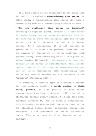
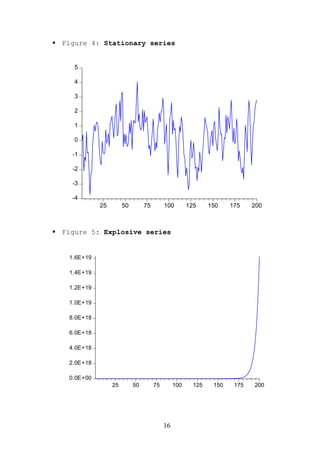
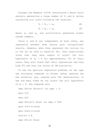
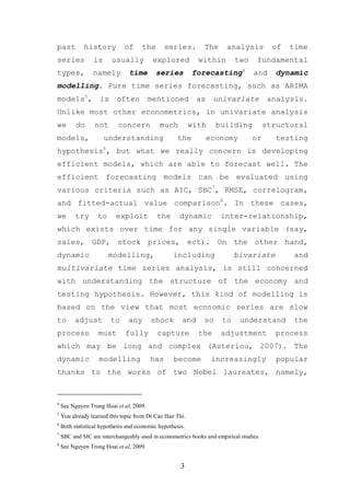
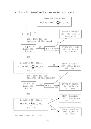
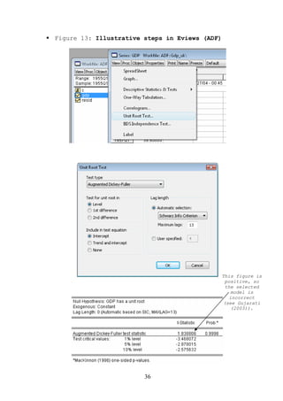
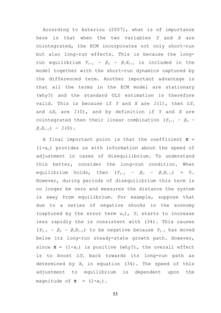
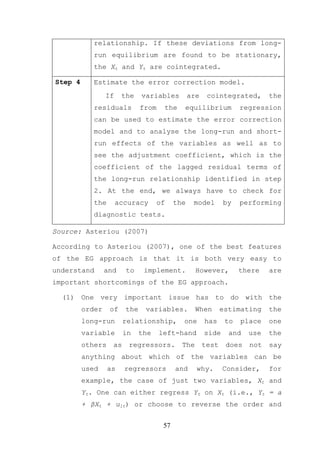
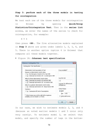
model and moving to the next model. This procedure is
illustrated in Figure 12. It needs to be stressed here
that, although useful, this procedure is not designed
to be applied in a mechanical fashion. Plotting the
data and observing the graph is sometimes very useful
because it can clearly indicate the presence or not of
deterministic regressors. However, this procedure is
the most sensible way to test for unit roots when the
form of the data-generating process is unknown.

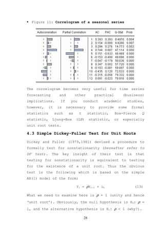
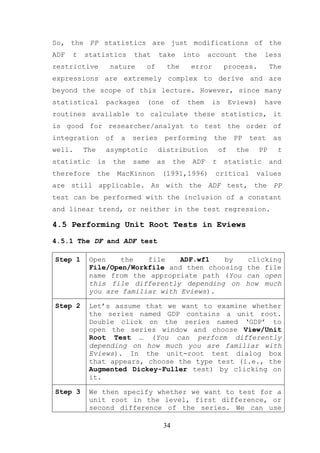
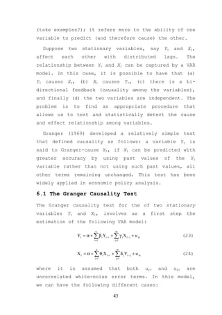
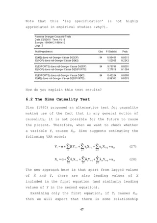
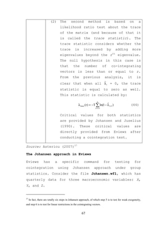
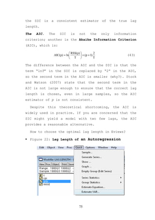
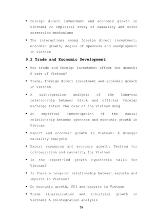
In practical studies, researchers use both the ADF
and the Phillips-Perron (PP) tests21. Because the
distribution theory that supporting the Dickey-Fuller
tests is based on the assumption of random error terms
[iid(0,σ2)], when using the ADF methodology we have to
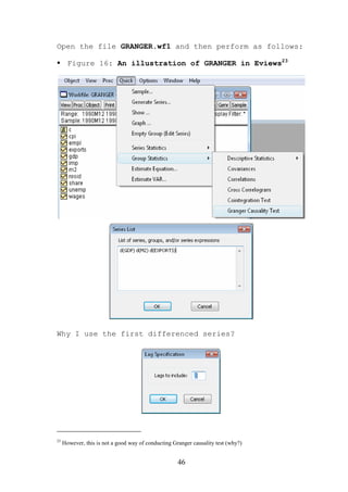
make sure that the error terms are uncorrelated and
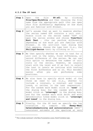
they really have a constant variance. Phillips and
Perron (1988) developed a generalization of the ADF
test procedure that allows for fairly mild assumptions
concerning the distribution of errors. The regression
for the PP test is similar to equation (15).

∆Yt = α + δYt-1 + et (20)

While the ADF test corrects for higher order serial
correlation by adding lagged differenced terms on the
right-hand side of the test equation, the PP test
makes a correction to the t statistic of the
coefficient δ from the AR(1) regression to account for
the serial correlation in et.

21
Eviews has a specific command for these tests.

32

Figure 12: Procedure for testing for unit roots

Estimate the model
p
∆Yt = α + γT + δYt −1 + ∑ β i ∆Yt −i + u t
i =1

NO STOP: Conclude
δ = 0? that there is no
unit root
YES: Test for the
presence of the trend
NO

is γ = 0? NO STOP: Conclude
given that δ = 0? that Yt has a
YES
δ = 0? unit root

YES

Estimate the model STOP: Conclude
p NO
∆Yt = α + δYt −1 + ∑ β i ∆Yt −i + u t that there is no
i =1 unit root
is δ = 0?

YES: Test for the NO
presence of the constant

is α = 0? NO STOP: Conclude
given that δ = 0? that Yt has a
YES
δ = 0? unit root

YES
STOP: Conclude
that there is no
Estimate the model NO unit root
p
∆Yt = δYt −1 + ∑ β i ∆Yt −i + u t
i =1

is δ = 0?
YES STOP: Conclude
that Yt has a
unit root

33

So, the PP statistics are just modifications of the
ADF t statistics that take into account the less
restrictive nature of the error process. The
expressions are extremely complex to derive and are
beyond the scope of this lecture. However, since many
statistical packages (one of them is Eviews) have
routines available to calculate these statistics, it
is good for researcher/analyst to test the order of
integration of a series performing the PP test as
well. The asymptotic distribution of the PP t
statistic is the same as the ADF t statistic and
therefore the MacKinnon (1991,1996) critical values
are still applicable. As with the ADF test, the PP
test can be performed with the inclusion of a constant
and linear trend, or neither in the test regression.

4.5 Performing Unit Root Tests in Eviews

4.5.1 The DF and ADF test

Step 1 Open the file ADF.wf1 by clicking
File/Open/Workfile and then choosing the file
name from the appropriate path (You can open
this file differently depending on how much
you are familiar with Eviews).

Step 2 Let’s assume that we want to examine whether
the series named GDP contains a unit root.
Double click on the series named ‘GDP’ to
open the series window and choose View/Unit
Root Test … (You can perform differently
depending on how much you are familiar with
Eviews). In the unit-root test dialog box
that appears, choose the type test (i.e., the
Augmented Dickey-Fuller test) by clicking on
it.

Step 3 We then specify whether we want to test for a
unit root in the level, first difference, or
second difference of the series. We can use

34

this option to determine the number of unit
roots in the series. However, we usually
start with the level and if we fail to reject
the test in levels we continue with testing
the first difference and so on. This becomes
easier after you are performing some
practices.

Step 4 We also have to specify which model of the
three ADF models we wish to use (i.e.,
whether to include a constant, a constant and
linear trend, or neither in the test
regression). For the model given by equation
(17) click on ‘none’ in the dialog box; for
the model given by equation (18) click on
‘intercept’ in the dialog box; and for the
model given by equation (19) click on
‘intercept and trend’ in the dialog box;

Step 5 Finally, we have to specify the number of
lagged dependent variables to be included in
the model in order to correct the presence of
serial correlation. In practice, we just
click the ‘automatic selection’ on the ‘lag
length’ dialog box.

Step 6 Having specified these options, click <OK> to
carry out the test. Eviews reports the test
statistic together with the estimated test
regression.

Step 7 We reject the null hypothesis of a unit root
against the one-sided alternative if the ADF
statistic is less than (lies to the left of)
the critical value, and we conclude that the
series is stationary.

Step 8 After running a unit root test, we should
examine the estimated test regression
reported by Eviews, especially if unsure
about the lag structure or deterministic
trend in the series. We may want to rerun the
test equation with a different selection of
right-hand variables (add or delete the
constant, trend, or lagged differences) or
lag order.


35

Figure 13: Illustrative steps in Eviews (ADF)

This figure is
positive, so
the selected
model is
incorrect
(see Gujarati
(2003)).

36

4.5.2 The PP test

Step 1 Open the file PP.wf1 by clicking
File/Open/Workfile and then choosing the file
name from the appropriate path (You can open
this file differently depending on how much
you are familiar with Eviews).

Step 2 Let’s assume that we want to examine whether
the series named GDP contains a unit root.
Double click on the series named ‘GDP’ to
open the series window and choose View/Unit
Root Test … (You can perform differently
depending on how much you are familiar with
Eviews). In the unit-root test dialog box
that appears, choose the type test (i.e., the
Phillipd-Perron test) by clicking on it.

Step 3 We then specify whether we want to test for a
unit root in the level, first difference, or
second difference of the series. We can use
this option to determine the number of unit
roots in the series. However, we usually
start with the level and if we fail to reject
the test in levels we continue with testing
the first difference and so on. This becomes
easier after you are performing some
practices.

Step 4 We also have to specify which model of the
three we need to use (i.e., whether to
include a constant, a constant and linear
trend, or neither in the test regression).
For the random walk model click on ‘none’ in
the dialog box; for the random with drift
model click on ‘intercept’ in the dialog box;
and for the random walk with drift and with
deterministic trend model click on ‘intercept
and trend’ in the dialog box.

Step 5 Finally, for the PP test we specify the lag
truncation to compute the Newey-West
heteroskedasticity and autocorrelation (HAV)22
consistent estimate of the spectrum at zero

22
This is already mentioned in the Basic Econometrics course, Serial Correlation topic.

37

frequency.

Step 6 Having specified these options, click <OK> to
carry out the test. Eviews reports the test
statistic together with the estimated test
regression.

Step 7 We reject the null hypothesis of a unit root
against the one-sided alternative if the ADF
statistic is less than (lies to the left of)
the critical value, and we conclude that the
series is stationary.


Figure 14: Illustrative steps in Eviews (PP)

This figure is
positive, so
the selected
model is
incorrect
(see Gujarati
(2003)).

38

5. VECTOR AUTOREGRESSIVE MODELS

According to Asteriou (2007), it is quite common in
economics to have models where some variables are not
only explanatory variables for a given dependent
variable, but they are also explained by the variables
that they are used to determine. In those cases, we
have models of simultaneous equations, in which it is
necessary to clearly identify which are the endogenous
and which are the exogenous or predetermined
variables. The decision regarding such a
differentiation among variables was heavily criticized
by Sims (1980).

According to Sims (1980), if there is simultaneity
among a number of variables, then all these variables
should be treated in the same way. In other words,
these should be no distinction between endogenous and
exogenous variables. Therefore, once this distinction
is abandoned, all variables are treated as endogenous.
This means that in its general reduced form, each
equation has the same set of regressors which leads to
the development of the VAR models.

The VAR model is defined as follow. Suppose we have
two series, in which Yt is affected by not only its
past values but current and past values of Xt, and
simultaneously, Xt is affected by not only its past
values but current and past values of Yt. This simple
bivariate VAR model is given by:

Yt = β10 - β12Xt + γ11Yt-1 + γ12Xt-1 + uyt (21)

Xt = β20 - β21Yt + γ21Yt-1 + γ22Xt-1 + uxt (22)

39

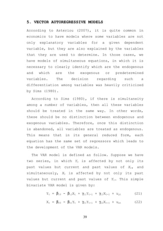
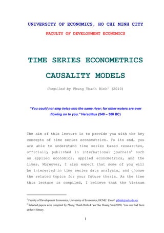
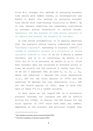
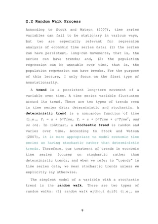
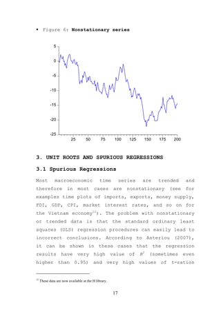
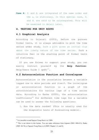
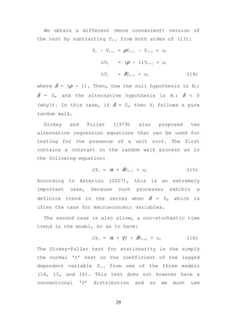
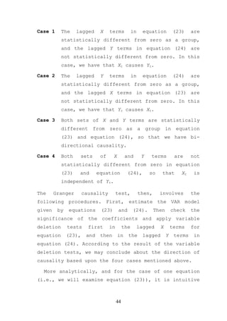
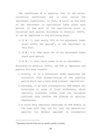
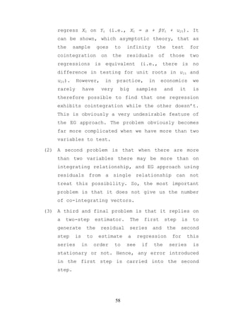
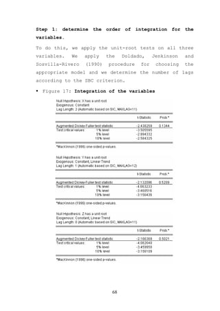
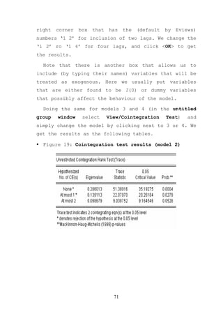
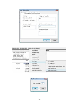
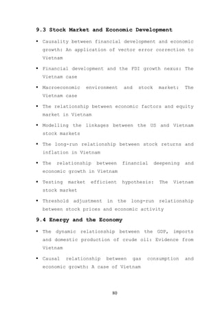
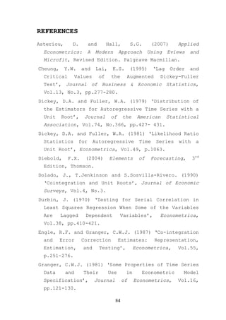
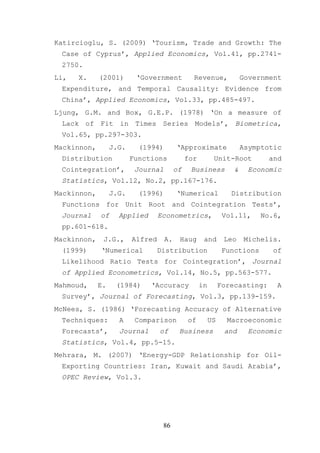
where we assume that both Yt and Xt are stationary and
uyt and uxt are uncorrelated white-noise error terms.
These equations are not reduced-form equations since
Yt has a contemporaneous impact on Xt, and Xt has a
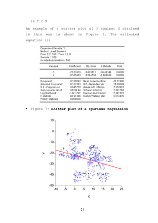
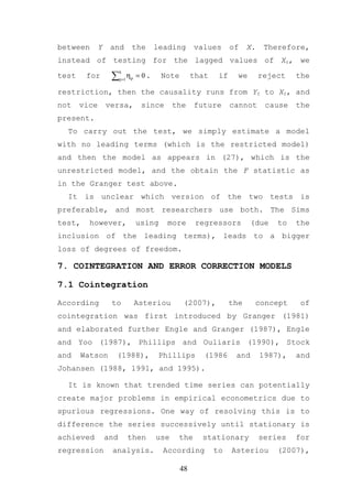
contemporaneous impact on Yt. The illustrative example
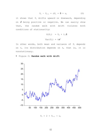
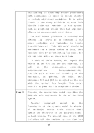
is presented in Figure 15 (open the file VAR.wf1).

Figure 15: An illustration of VAR in Eviews

Vector Autoregression Estimates
Date: 02/20/10 Time: 15:46
Sample (adjusted): 1975Q3 1997Q4
Included observations: 90 after adjustments
Standard errors in ( ) & t-statistics in [ ]

GDP M2

GDP(-1) 1.230362 -0.071108
(0.10485) (0.09919)
[11.7342] [-0.71691]
GDP(-2) -0.248704 0.069167
(0.10283) (0.09728)
[-2.41850] [0.71103]
M2(-1) 0.142726 1.208942
(0.11304) (0.10693)

40

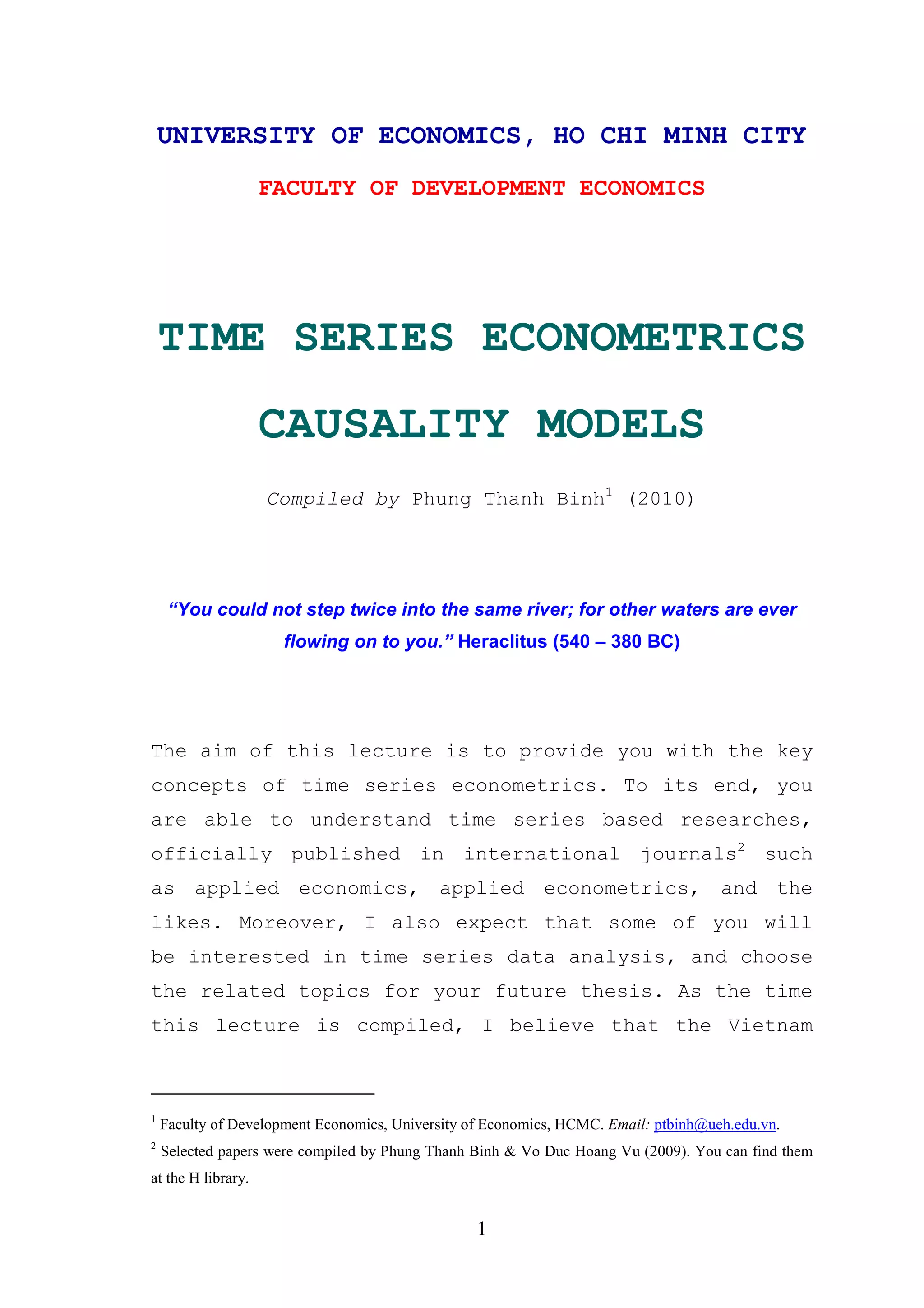
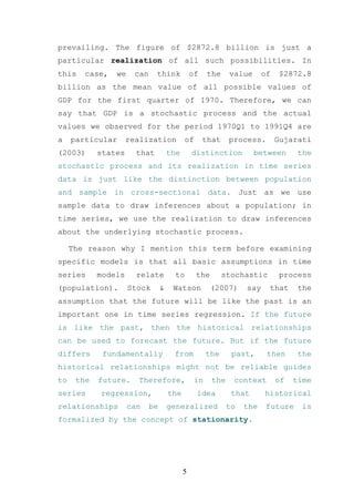
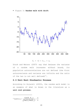
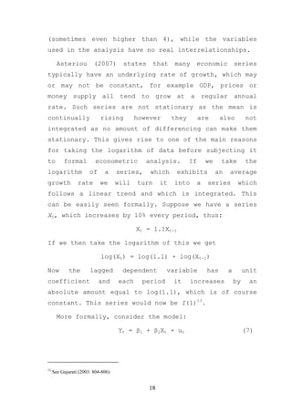
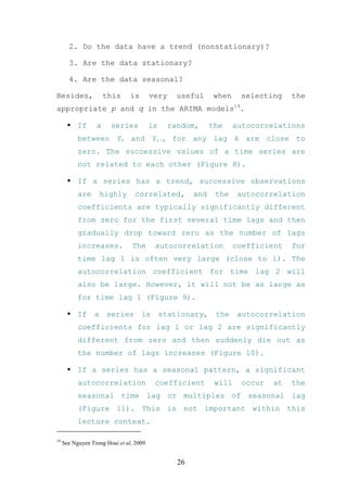
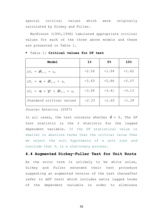
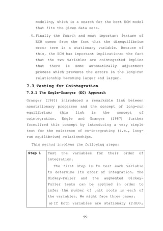
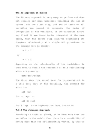
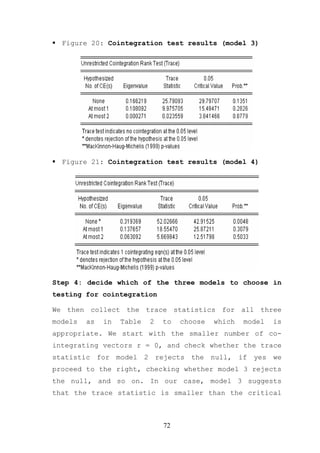
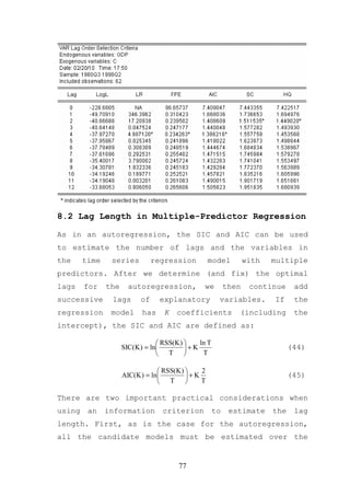
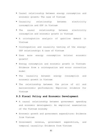
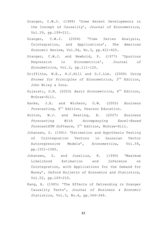
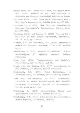
[1.26267] [11.3063]
M2(-2) -0.087270 -0.206244
(0.11599) (0.10972)
[-0.75237] [-1.87964]
C 4.339620 8.659425
(3.02420) (2.86077)
[1.43497] [3.02696]

R-squared 0.999797 0.998967
Adj. R-squared 0.999787 0.998918
Sum sq. resids 6000.811 5369.752
S.E. equation 8.402248 7.948179
F-statistic 104555.2 20543.89
Log likelihood -316.6973 -311.6972
Akaike AIC 7.148828 7.037716
Schwarz SC 7.287707 7.176594
Mean dependent 967.0556 509.1067
S.D. dependent 576.0331 241.6398

Determinant resid covariance 4459.738
Determinant resid covariance 3977.976
Log likelihood -628.3927
Akaike information criterion 14.18650
Schwarz criterion 14.46426

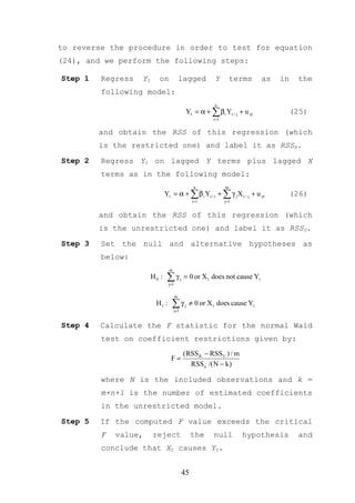
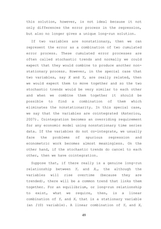
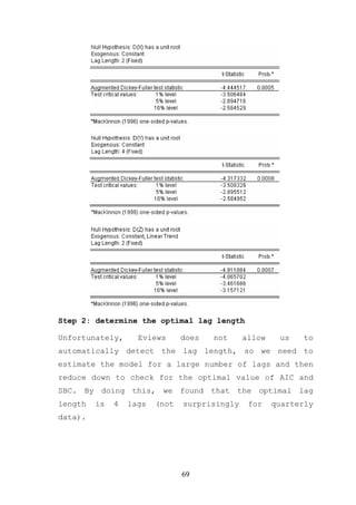
According to Asteriou (2007), the VAR model has some
good characteristics. First, it is very simple because
we do not have to worry about which variables are
endogenous or exogenous. Second, estimation is very
simple as well, in the sense that each equation can be
estimated with the usual OLS method separately. Third,
forecasts obtained from VAR models are in most cases
better than those obtained from the far more complex
simultaneous equation models (see Mahmoud, 1984;
McNees, 1986). Besides forecasting purposes, VAR
models also provide framework for causality tests,
which will be presented shortly in the next section.

However, on the other hand the VAR models have faced
severe criticism on various different points.

41

According to Asteriou (2007), the VAR models have been
criticised by the following aspects. First, they are
a-theoretic since they are not based on any economic
theory. Since initially there are no restrictions on
any of the parameters under estimation, in effect
‘everything causes everything’. However, statistical
inference is often used in the estimated models so
that some coefficients that appear to be insignificant
can be dropped, in order to lead models that might
have an underlying consistent theory. Such inference
is normally carried out using what are called
causality tests. Second, they are criticised due to
the loss of degrees of freedom. Thus, if the sample
size is not sufficiently large, estimating that large
a number of parameters, say, a three-variable VAR
model with 12 lags for each, will consume many degrees
of freedom, creating problems in estimation. Third,
the obtained coefficients of the VAR models are
difficult to interpret since they totally lack any
theoretical background.

If you are interested in VAR models, you can find
additional readings from the econometrics textbooks
about time series data, listed in the references of
this lecture.

6. CAUSALITY TESTS

According to Asteriou (2007), one of the good features
of VAR models is that they allow us to test the
direction of causality. Causality in econometrics is
somewhat different to the concept in everyday use

42

(take examples?); it refers more to the ability of one
variable to predict (and therefore cause) the other.

Suppose two stationary variables, say Yt and Xt,
affect each other with distributed lags. The
relationship between Yt and Xt can be captured by a VAR
model. In this case, it is possible to have that (a)
Yt causes Xt, (b) Xt causes Yt, (c) there is a bi-
directional feedback (causality among the variables),
and finally (d) the two variables are independent. The
problem is to find an appropriate procedure that
allows us to test and statistically detect the cause
and effect relationship among variables.

Granger (1969) developed a relatively simple test
that defined causality as follows: a variable Yt is
said to Granger-cause Xt, if Xt can be predicted with
greater accuracy by using past values of the Yt
variable rather than not using such past values, all
other terms remaining unchanged. This test has been
widely applied in economic policy analysis.

6.1 The Granger Causality Test

The Granger causality test for the of two stationary
variables Yt and Xt , involves as a first step the
estimation of the following VAR model:
n m
Yt = α + ∑ β i Yt −i + ∑ γ j X t − j + u yt (23)
i =1 j=1

n m
X t = α + ∑ θ i X t −i + ∑ δ j Yt − j + u xt (24)
i =1 j=1

where it is assumed that both uyt and uxt are
uncorrelated white-noise error terms. In this model,
we can have the following different cases:

43

Case 1 The lagged X terms in equation (23) are
statistically different from zero as a group,
and the lagged Y terms in equation (24) are
not statistically different from zero. In this
case, we have that Xt causes Yt.

Case 2 The lagged Y terms in equation (24) are
statistically different from zero as a group,
and the lagged X terms in equation (23) are
not statistically different from zero. In this
case, we have that Yt causes Xt.

Case 3 Both sets of X and Y terms are statistically
different from zero as a group in equation
(23) and equation (24), so that we have bi-
directional causality.

Case 4 Both sets of X and Y terms are not
statistically different from zero in equation
(23) and equation (24), so that Xt is
independent of Yt.

The Granger causality test, then, involves the
following procedures. First, estimate the VAR model
given by equations (23) and (24). Then check the
significance of the coefficients and apply variable
deletion tests first in the lagged X terms for
equation (23), and then in the lagged Y terms in
equation (24). According to the result of the variable
deletion tests, we may conclude about the direction of
causality based upon the four cases mentioned above.

More analytically, and for the case of one equation
(i.e., we will examine equation (23)), it is intuitive

44

to reverse the procedure in order to test for equation
(24), and we perform the following steps:

Step 1 Regress Yt on lagged Y terms as in the
following model:
n
Yt = α + ∑ β i Yt − j + u yt (25)
i =1

and obtain the RSS of this regression (which
is the restricted one) and label it as RSSR.
Step 2 Regress Yt on lagged Y terms plus lagged X
terms as in the following model:
n m
Yt = α + ∑ β i Yt −i + ∑ γ j X t − j + u yt (26)
i =1 j=1

and obtain the RSS of this regression (which
is the unrestricted one) and label it as RSSU.

Step 3 Set the null and alternative hypotheses as
below:
m
H0 : ∑γ
j=1
j = 0 or X t does not cause Yt

m
H1 : ∑γ j=1
j ≠ 0 or X t does cause Yt

Step 4 Calculate the F statistic for the normal Wald
test on coefficient restrictions given by:
(RSS R − RSS U ) / m
F=
RSS u /( N − k )

where N is the included observations and k =
m+n+1 is the number of estimated coefficients
in the unrestricted model.

Step 5 If the computed F value exceeds the critical
F value, reject the null hypothesis and
conclude that Xt causes Yt.

45

Open the file GRANGER.wf1 and then perform as follows:

Figure 16: An illustration of GRANGER in Eviews23

Why I use the first differenced series?

23
However, this is not a good way of conducting Granger causality test (why?)

46

Note that this ‘lag specification’ is not highly
appreciated in empirical studies (why?).

How do you explain this test results?

6.2 The Sims Causality Test

Sims (1980) proposed an alternative test for causality
making use of the fact that in any general notion of
causality, it is not possible for the future to cause
the present. Therefore, when we want to check whether
a variable Yt causes Xt, Sims suggests estimating the
following VAR model:
n m k
Yt = α + ∑ β i Yt −i + ∑ γ j X t − j + ∑ ηρ X t +ρ + u yt (27)
i =1 j=1 ρ =1

n m k
X t = α + ∑ θ i X t −i + ∑ δ j Yt − j + ∑ λ ρ Yt +ρ + u xt (28)
i =1 j=1 ρ =1

The new approach here is that apart from lagged values
of X and Y, there are also leading values of X
included in the first equation (and similarly leading
values of Y in the second equation).
Examining only the first equation, if Yt causes Xt,
then we will expect that there is some relationship

47

between Y and the leading values of X. Therefore,
instead of testing for the lagged values of Xt, we

∑
k
test for ρ =1
ηρ = 0 . Note that if we reject the

restriction, then the causality runs from Yt to Xt, and
not vice versa, since the future cannot cause the
present.
To carry out the test, we simply estimate a model
with no leading terms (which is the restricted model)
and then the model as appears in (27), which is the
unrestricted model, and the obtain the F statistic as
in the Granger test above.
It is unclear which version of the two tests is
preferable, and most researchers use both. The Sims
test, however, using more regressors (due to the
inclusion of the leading terms), leads to a bigger
loss of degrees of freedom.

7. COINTEGRATION AND ERROR CORRECTION MODELS

7.1 Cointegration

According to Asteriou (2007), the concept of
cointegration was first introduced by Granger (1981)
and elaborated further Engle and Granger (1987), Engle
and Yoo (1987), Phillips and Ouliaris (1990), Stock
and Watson (1988), Phillips (1986 and 1987), and
Johansen (1988, 1991, and 1995).

It is known that trended time series can potentially
create major problems in empirical econometrics due to
spurious regressions. One way of resolving this is to
difference the series successively until stationary is
achieved and then use the stationary series for
regression analysis. According to Asteriou (2007),

48

this solution, however, is not ideal because it not
only differences the error process in the regression,
but also no longer gives a unique long-run solution.

If two variables are nonstationary, then we can
represent the error as a combination of two cumulated
error process. These cumulated error processes are
often called stochastic trends and normally we could
expect that they would combine to produce another non-
stationary process. However, in the special case that
two variables, say X and Y, are really related, then
we would expect them to move together and so the two
stochastic trends would be very similar to each other
and when we combine them together it should be
possible to find a combination of them which
eliminates the nonstationarity. In this special case,
we say that the variables are cointegrated (Asteriou,
2007). Cointegration becomes an overriding requirement
for any economic model using nonstationary time series
data. If the variables do not co-integrate, we usually
face the problems of spurious regression and
econometric work becomes almost meaningless. On the
other hand, if the stochastic trends do cancel to each
other, then we have cointegration.

Suppose that, if there really is a genuine long-run
relationship between Yt and Xt , the although the
variables will rise overtime (because they are
trended), there will be a common trend that links them
together. For an equilibrium, or long-run relationship
to exist, what we require, then, is a linear
combination of Yt and Xt that is a stationary variable
(an I(0) variable). A linear combination of Yt and Xt

49

can be directly taken from estimating the following
regression:

Yt = β1 + β2Xt + ut (29)

And taking the residuals:

u t = Yt − β1 − β 2 X t
ˆ ˆ ˆ (30)

ˆ
If u t ~ I(0), then the variables Yt and Xt are said to
be co-integrated.

Importantly, based on the previous studies, we can
draw the general procedure for nonstationary series
analysis as follows:

(1) If (two) nonstationary variables are integrated of
the same order, but not co-integrated, we should
apply VAR models for the differenced series. These
models just provide short-run relationships
between them. This is widely called the “Standard
version of Granger causality” (Section 6.1).

the same order, and co-integrated, we cannot apply
the standard Granger causality test. The existence
of co-integrating relationships between variables
suggests that there must be Granger causality in
at least one direction. However, it does not
indicate the direction of temporal causality
between the variables. To determine the direction
of causation, we must examine the error correction
mechanism (ECM) model. The ECM enables us to
distinguish between ‘short-run’ and ‘long-run’
Granger causality. This is widely known as the
“Cointegration and Error Correction version of

50

Granger causality” (Section 7.2). We sometimes use
the term ‘cointegration and error correction
version of Granger causality’ and ECM
interchangeably.

the different orders, or non-cointegrated or
cointegrated of an arbitrary order, we cannot
apply either the standard Granger causality test
or the ECM. In these cases, it is often suggested
to employ the “Toda and Yamamoto version of
Granger causality”, or simply the Toda and
Yamamoto methodology, using the modified Wald
(MWALD) test statistic (see Mehrara, 2007).
Another method is “Bounds Test for Cointegration
within ARDL” developed by Pesaran et al. (2001)
(see Katircioglu, 2009). However, these are beyond
the scope of this lecture.

7.2 Error Correction Mechanism

According to Asteriou (2007), the concepts of
cointegration and the error correction mechanism
(hereafter refer to ECM) are very closely related. To
understand the ECM, it is better to think first of the
ECM as a convenient reparametrization of the general
linear autoregressive distributed lag (ARDL) model.

Consider the very simple dynamic ARDL model
describing the behaviour of Y in terms of X as
follows:

Yt = a0 + a1Yt-1 + γ0Xt + γ1Xt-1 + ut (31)

where ut ~ iid(0,σ2).

51

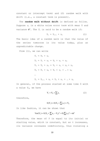
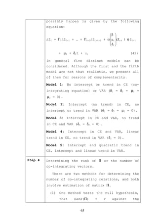
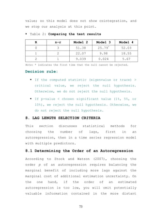
In this model24, the parameter γ0 denotes the short-
run reaction of Yt after a change in Xt. The long-run
effect is given when the model is in equilibrium
where:

Yt* = β 0 + β1 X *
t (32)

and for simplicity, we assume that:

X * = X t = X t −1 = ... = X t − p
t (33)

From (31), (32), and (33), we have:

Yt* = a 0 + a 1Yt* + γ 0 X * + γ 1X * + u t
t t

Yt* (1 − a 1 ) = a 0 + ( γ 0 + γ 1 )X * + u t
t

a0 γ + γ1 *
Yt* = + 0 Xt + u t
1 − a1 1 − a1

Yt* = β 0 + β1 X * + u t
t (34)

Therefore, the long-run elasticity between Y and X is
captured by β1=(γ0+γ1)/(1-a1). It is noted that, we need
to make the assumption that a1 < 1 (why?) in order
that the short-run model (31) converges to a long-run
solution.

The ECM can be rewritten as follows:

∆Yt = γ0∆Xt – (1-a)[Yt-1 – β0 – β1Xt-1] + ut (35)

∆Yt = γ0∆Xt – π[Yt-1 – β0 – β1Xt-1] + ut (36)

(please show that the ECM model (35) is the same as
the original model (31)?)

24
We can easily expand this model to a more general case for large numbers of lagged terms.

52

According to Asteriou (2007), what is of importance
here is that when the two variables Y and X are
cointegrated, the ECM incorporates not only short-run
but also long-run effects. This is because the long-
run equilibrium Yt-1 – β0 – β1Xt-1 is included in the
model together with the short-run dynamics captured by
the differenced term. Another important advantage is
that all the terms in the ECM model are stationary
(why?) and the standard OLS estimation is therefore
valid. This is because if Y and X are I(1), then ∆Yt
and ∆Xt are I(0), and by definition if Y and X are
cointegrated then their linear combination (Yt-1 – β0 –
β1Xt-1) ~ I(0).

A final important point is that the coefficient π =
(1-a1) provides us with information about the speed of
adjustment in cases of disequilibrium. To understand
this better, consider the long-run condition. When
equilibrium holds, then (Yt-1 – β0 – β1Xt-1) = 0.
However, during periods of disequilibrium this term is
no longer be zero and measures the distance the system
is away from equilibrium. For example, suppose that
due to a series of negative shocks in the economy
(captured by the error term ut), Yt starts to increase
less rapidly the is consistent with (34). This causes
(Yt-1 – β0 – β1Xt-1) to be negative because Yt-1 has moved
below its long-run steady-state growth path. However,
since π = (1-a1) is positive (why?), the overall effect
is to boost ∆Yt back towards its long-run path as
determined by Xt in equation (34). The speed of this
adjustment to equilibrium is dependent upon the
magnitude of π = (1-a1).

53

The coefficient π in equation (36) is the error-
correction coefficient and is also called the
adjustment coefficient. In fact, π tells us how much
of the adjustment to equilibrium takes place each
period, or how much of the equilibrium error is
corrected each period. According to Asteriou (2007),
it can be explained in the following ways:

1. If π ~ 1, then nearly 100% of the adjustment takes
place within the period25, or the adjustment is
very fast.

2. If π ~ 0.5, then about 50% of the adjustment takes
place each period.

3. If π ~ 0, then there seems to be no adjustment.

According to Asteriou (2007), the ECM is important and
popular for many reasons:

1. Firstly, it is a convenient model measuring the
correction from disequilibrium of the previous
period which has a very good economic implication.

2. Secondly, if we have cointegration, ECM models are
formulated in terms of first difference, which
typically eliminate trends from the variables
involved; they resolve the problem of spurious
regressions.

3. A third very important advantage of ECM models is
the ease with they can fit into the general-to-
specific (or Hendry) approach to econometric

25
Depending on the kind of data used, say, annually, quarterly, or monthly.

54

modeling, which is a search for the best ECM model
that fits the given data sets.

4. Finally the fourth and most important feature of
ECM comes from the fact that the disequilibrium
error term is a stationary variable. Because of
this, the ECM has important implications: the fact
that the two variables are cointegrated implies
that there is some automatically adjustment
process which prevents the errors in the long-run
relationship becoming larger and larger.

7.3 Testing for Cointegration
7.3.1 The Engle-Granger (EG) Approach

Granger (1981) introduced a remarkable link between
nonstationary processes and the concept of long-run
equilibrium; this link is the concept of
cointegration. Engle and Granger (1987) further
formulized this concept by introducing a very simple
test for the existence of co-integrating (i.e., long-
run equilibrium) relationships.

This method involves the following steps:

Step 1 Test the variables for their order of
integration.
The first step is to test each variable
to determine its order of integration. The
Dickey-Fuller and the augmented Dickey-
Fuller tests can be applied in order to
infer the number of unit roots in each of
the variables. We might face three cases:
a) If both variables are stationary (I(0)),

55

it is not necessary to proceed since
standard time series methods apply to
stationary variables.
b) If the variables are integrated of
different orders, it is possible to
conclude that they are not cointegrated.
c) If both variables are integrated of the
same order, we proceed with step two.

Step 2 Estimate the long-run (possible co-
integrating) relationship.
If the results of step 1 indicate that
both Xt and Yt are integrated of the same
order (usually I(1)) in economics, the next
step is to estimate the long-run equilibrium
relationship of the form:

Yt = β1 + β 2 X t + u t (37)

and obtain the residuals of this equation.
If there is no cointegration, the results
obtained will be spurious. However, if the
variables are cointegrated, OLS regression
yields consistent estimators for the co-
integrating parameter β 2 .
ˆ

Step 3 Check for (cointegration) the order of
integration of the residuals.
In order to determine if the variables
are actually cointegrated, denote the
estimated residual sequence from the
ˆ ˆ
equation by u t . Thus, u t is the series of the
estimated residuals of the long-run

56

relationship. If these deviations from long-
run equilibrium are found to be stationary,
the Xt and Yt are cointegrated.

Step 4 Estimate the error correction model.
If the variables are cointegrated, the
residuals from the equilibrium regression
can be used to estimate the error correction
model and to analyse the long-run and short-
run effects of the variables as well as to
see the adjustment coefficient, which is the
coefficient of the lagged residual terms of
the long-run relationship identified in step
2. At the end, we always have to check for
the accuracy of the model by performing
diagnostic tests.


According to Asteriou (2007), one of the best features
of the EG approach is that it is both very easy to
understand and to implement. However, there are
important shortcomings of the EG approach.

(1) One very important issue has to do with the
order of the variables. When estimating the
long-run relationship, one has to place one
variable in the left-hand side and use the
others as regressors. The test does not say
anything about which of the variables can be
used as regressors and why. Consider, for
example, the case of just two variables, Xt and
Yt. One can either regress Yt on Xt (i.e., Yt = a
+ βXt + u1t) or choose to reverse the order and

57

regress Xt on Yt (i.e., Xt = a + βYt + u2t). It
can be shown, which asymptotic theory, that as
the sample goes to infinity the test for
cointegration on the residuals of those two
regressions is equivalent (i.e., there is no
difference in testing for unit roots in u1t and
u2t). However, in practice, in economics we
rarely have very big samples and it is
therefore possible to find that one regression
exhibits cointegration while the other doesn’t.
This is obviously a very undesirable feature of
the EG approach. The problem obviously becomes
far more complicated when we have more than two
variables to test.

(2) A second problem is that when there are more
than two variables there may be more than on
integrating relationship, and EG approach using
residuals from a single relationship can not
treat this possibility. So, the most important
problem is that it does not give us the number
of co-integrating vectors.

(3) A third and final problem is that it replies on
a two-step estimator. The first step is to
generate the residual series and the second
step is to estimate a regression for this
series in order to see if the series is
stationary or not. Hence, any error introduced
in the first step is carried into the second
step.

58

The EG approach in Eviews

The EG test approach is very easy to perform and does
not require any more knowledge regarding the use of
Eviews. For the first step, ADF and PP tests on all
variables are needed to determine the order of
integration of the variables. If the variables (let’s
say X and Y) are found to be integrated of the same
order, then the second step involves estimating the
long-run relationship with simple OLS procedure. So
the command here is simply:

ls X c Y

or

ls Y c X

depending on the relationship of the variables. We
then need to obtain the residuals of this relationship
which are given by:

genr res1=resid

The third step (the actual test for cointegration) is
a unit root test on the residuals, the command for
which is:

adf res1

for no lags, or

adf(4) res1

for 4 lags in the augmentation term, and so on.

7.3.2 The Johansen Approach

According to Asteriou (2007), if we have more than two
variables in the model, then there is a possibility of
having more than one co-integrating vector. By this we

59

mean that the variables in the model might form
several equilibrium relationships. In general, for n
number of variables, we can have only up to n-1 co-
integrating vectors.

Having n > 2 and assuming that only one co-
integrating relationship exists, where there are
actually more than one, is a very serious problem that
cannot be resolved by the EG single-equation approach.
Therefore, an alternative to the EG approach is needed
and this is the Johansen approach26 for multiple
equations.

In order to present this approach, it is useful to
extend the single-equation error correction model to a
multivariate one. Let’s assume that we have three
variables, Yt, Xt and Wt, which can all be endogenous,
i.e., we have that (using matrix notation for Zt =
[Yt,Xt,Wt])

Zt = A1Zt-1 + A2Zt-2 + … + AkZt-k + ut (37)

which is comparable to the single-equation dynamic
model for two variables Yt and Xt given in (31). Thus,
it can be reformulated in a vector error correction
model (VECM) as follows:

∆Zt = Γ1∆Zt-1 + Γ2∆Zt-2 + … + Γk-1∆Zt-k-1 + ΠZt-1 + ut (38)

where the matrix Π contains information regarding the
long-run relationships. We can decompose Π = αβ’ where
α will include the speed of adjustment to equilibrium

26
For clearer, please read Li, X. (2001) ‘Government Revenue, Government Expenditure, and Temporal
Causality: Evidence from China’, Applied Economics, Vol.33, pp.485-497.

60

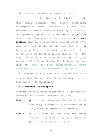
coefficients, while β’ will be the long-run matrix of
coefficients.

Therefore, the β’Zt-1 term is equivalent to the error
correction term (Yt-1 – β0 – β1Xt-1) in the single-
equation case, except that now β’Zt-1 contains up to (n
– 1) vectors in a multivariate framework.

For simplicity, we assume that k = 2, so that we
have only two lagged terms, and the model is then the
following:

 ∆Yt   ∆Yt −1   Yt −1 
     
 ∆X t  = Γ1  ∆X t −1  + Π X t −1  + e t (38)
   ∆W  W 
 ∆Wt   t −1   t −1 

or

 ∆Yt   ∆Yt −1   α11 α 12  Y 
      β11 β 21 β 31  t −1 
 ∆X t  = Γ1  ∆X t −1  +  α 21 α 22 
  X t −1  + e t
 (39)
 ∆W   ∆W   α α  β12 β 22 β 32  W 
 t   t −1   31 32   t −1 

Let us now analyse only the error correction part of
the first equation (i.e., for ∆Yt on the left-hand
side) which gives:

Π1Zt-1 = ([α11β11 + α12β12][α11β21 + α12β22]

 Yt −1 
 
[α11β31 + α12β32])  X t −1  (40)
W 
 t −1 

Equation (40) can be rewritten as:

Π1Zt-1 = α11(β11Yt-1 + β21Xt-1 + β31Wt-1) +

α12(β12Yt-1 + β22Xt-1 + β32Wt-1) (41)

61

which shows clearly the two co-integrating vectors
with their respective speed of adjustment terms α11 and
α12.

What are advantages of the multiple equation
(Johansen) approach?

From the multiple equation approach we can obtain
estimates for both co-integrating vectors (41),
while the simple equation we have only a linear
combination of the two long-run relationships.

Even if there is only one co-integrating
relationship (for example the first only) rather
than two, with the multiple equation approach we
can calculate all three differing speeds of
adjustment coefficients (α11 α21 α31)’.

Only when α21 = α31 = 0, and only one co-
integrating relationship exists, can we then say
that the multiple equation method is the same
(reduces to) as the single equation approach, and
therefore, there is no loss from not modelling the
determinants of ∆Xt and ∆Wt. Here, it is good to
mention as well that when α21 = α31 = 0, is
equivalent to Xt and Wt being weakly exogenous.

Therefore, only when all right-hand variables in a
single equation are weakly exogenous does the single-
equation approach provide the same result as a
multivariate equation approach.

62

Causality models

Recommended

Recommended

More Related Content

What's hot

What's hot (20)

Viewers also liked

Viewers also liked (14)

Similar to Causality models

Similar to Causality models (20)

Causality models