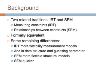
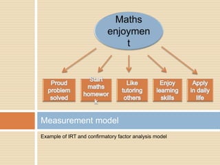
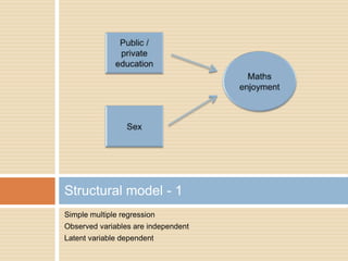
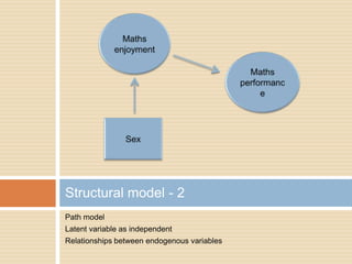
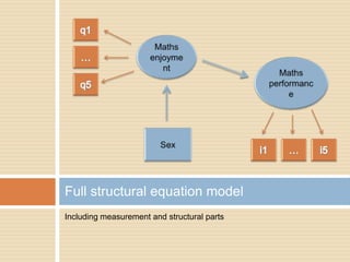
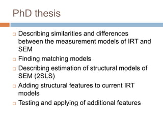
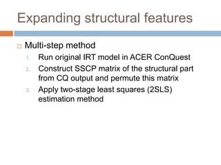
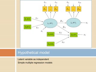
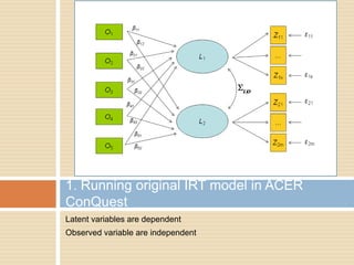
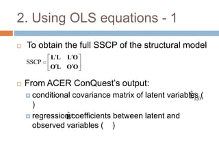
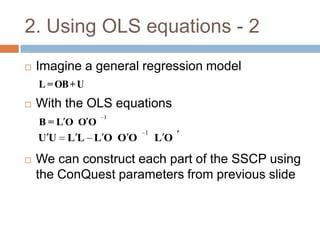
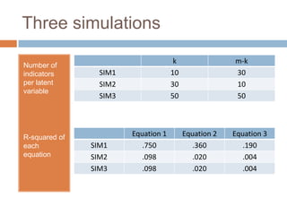
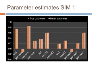
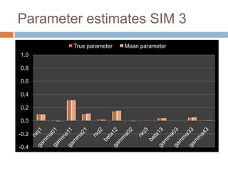
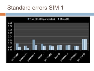
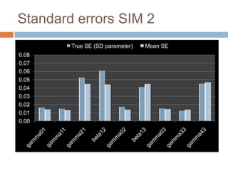
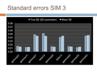
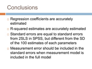
BRIDGING THE GAP
BETWEEN ITEM
RESPONSE THEORY AND
STRUCTURAL EQUATION
MODELLING
PhD thesis Eveline Gebhardt
Background
   Two related traditions: IRT and SEM
     Measuring  constructs (IRT)
     Relationships between constructs (SEM)

   Formally equivalent
   Some remaining differences:
     IRTmore flexibility measurement models
     And in data structure and guessing parameter

     SEM more flexible structural models

     SEM quicker
Measurement model
Example of IRT and confirmatory factor analysis model
Structural model - 1
Simple multiple regression
Observed variables are independent
Latent variable dependent
Structural model - 2
Path model
Latent variable as independent
Relationships between endogenous variables
Full structural equation model
Including measurement and structural parts
PhD thesis
   Describing similarities and differences
    between the measurement models of IRT and
    SEM
   Finding matching models
   Describing estimation of structural models of
    SEM (2SLS)
   Adding structural features to current IRT
    models
   Testing and applying of additional features
Expanding structural features
   Multi-step method
    1.   Run original IRT model in ACER ConQuest
    2.   Construct SSCP matrix of the structural part
         from CQ output and permute this matrix
    3.   Apply two-stage least squares (2SLS)
         estimation method
Hypothetical model
Latent variable as independent
Simple multiple regression models
1. Running original IRT model in ACER
ConQuest
Latent variables are dependent
Observed variable are independent
2. Using OLS equations - 1
   To obtain the full SSCP of the structural model
           LL   LO
    SSCP
           OL OO

   From ACER ConQuest’s output:
     conditional                                      ˆc
                    covariance matrix of latent variablesO(
                                                        L|
      )
                ˆ
     regression c
               B coefficients between latent and
      observed variables ( )
2. Using OLS equations - 2
   Imagine a general regression model
    L = OΒ + U
   With the OLS equations
                 1
    Β=LO OO
                      1
    UU    LL LO OO        LO

   We can construct each part of the SSCP using
    the ConQuest parameters from previous slide
2. Using OLS equations - 3
    ˆ
L O Bc O O


OL         ˆ
       O O Bc


L'L = U ¢ + L'O (O'O ) (L ¢ )¢
                      -1
        U                 O
                           ¢
         U ˆ ˆ
     = U ¢ + Bc (Bc (O ¢ ))
                       O

         U ˆ       O ˆ
     = U ¢ + Bc (O ¢ )B c¢
       ˆ                 ˆ     O ˆ
     = Σ cL O (N - K ) + Bc (O ¢ )B c¢
       (             )
                  é                        ù
                  UU ˆ      O ˆ    ˆ
        éL¢ L¢ ù ê ¢ + Bc (O¢ )Bc¢ Bc (O¢ )ú
           L O                           O
 SSCP = ê      ú= ê                        ú
        ê ¢ O¢ ú ê
        ë L
         O    Oû
                  ê
                  ë     O ˆ
                     (O¢ )Bc¢        O¢ ú
                                        O úû
3. Permuting the original SSCP
   Latent and observed variables are redefined
    as endogenous (Y) and exogenous (X)
    variables
     Endogenous       variables are being explained by the
      model (l1, l2, o5)
     Exogenous variables only explain other variables
      (o1, o2, o3, o4)
   And *then reordered using the following
            Y'Y Y'X
    SSCP
    structure
            X'Y X'X
4. Applying 2SLS - 1
   Two-stage least squares is the most common
    estimation method for path models
         m is for the current equation
         A is for variables included in m


     A             1      A        A   A              A              1
    Ym X X X           X Ym       Ym X m    γm
                                             A
                                                     Ym X X X            X Ym
              A  A
            X m Ym                 A  A
                                  Xm Xm     βm
                                             A
                                                              A
                                                            X m Ym
                                                     1
               A              1      A      A    A        A              1
    γ   A
        m
             Y X XX
               m                  XY m     Y X
                                            m    m       Ym X X X            X Ym
    β   A
        m
                         A  A
                       X m Ym               A  A
                                           Xm Xm               A
                                                             X m Ym
4. Applying 2SLS - 2
   Additional estimates
     Standard         errors
                                                             1
                   A                 1    A         A    A
               2
                   Y X XX
                   m                     XY
                                          m        Y X
                                                    m    m
      S    s
                              A  A                  A  A
                            X m Ym                 Xm Xm

     Explained         variance

                                ee
      R2   1                                   2
                            2       1
                       Ym       N         Ym
Simulation study
   Part 1 - estimated structural parameters were
    evaluated by comparing them with the true
    structural parameters and their standard error
   Part 2 - the same structural parameters were
    compared with parameters as estimated by the
    2SLS procedure in SPSS and a path model
    procedure in Mplus.
   Part 3 - results from the full model, including the
    measurement model, were compared between the
    multi-step approach and a structural equation
    model using Mplus
Simulation study – part 1
   Generate student responses using known
    (true) parameters of a hypothetical model (100
    replications)
   Running original IRT model in ACER
    ConQuest
   Applying multi-step method
   Compare average estimates with true
    parameters
General model
Number of indicators and values of parameters can be manipulated for
each analysis
,


        Set of three equations
           Equation 1
    ,


           Equation 2


           Equation 3
Three simulations
                                      k                m-k
Number of
indicators       SIM1                10                30
per latent       SIM2                30                10
variable
                 SIM3                50                50


R-squared of            Equation 1        Equation 2   Equation 3
each           SIM1        .750              .360         .190
equation       SIM2        .098              .020         .004
               SIM3        .098              .020         .004
Parameter estimates SIM 1
        True parameter   Mean parameter
1.0

0.8

0.6

0.4

0.2

0.0

-0.2

-0.4
Parameter estimates SIM 2
        True parameter   Mean parameter
1.0

0.8

0.6

0.4

0.2

0.0

-0.2

-0.4
Parameter estimates SIM 3
        True parameter   Mean parameter
1.0

0.8

0.6

0.4

0.2

0.0

-0.2

-0.4
Standard errors SIM 1
        True SE (SD parameter)   Mean SE
0.08
0.07
0.06
0.05
0.04
0.03
0.02
0.01
0.00
Standard errors SIM 2
        True SE (SD parameter)   Mean SE
0.08
0.07
0.06
0.05
0.04
0.03
0.02
0.01
0.00
Standard errors SIM 3
        True SE (SD parameter)   Mean SE
0.08
0.07
0.06
0.05
0.04
0.03
0.02
0.01
0.00
Conclusions
   Regression coefficients are accurately
    estimated
   R-squared estimates are accurately estimated
   Standard errors are equal to standard errors
    from 2SLS in SPSS, but different from the SD
    of the 100 estimates of each parameters
   Measurement error should be included in the
    standard errors when measurement model is
    included in the full model

Thesis Multi Step Method 111006

  • 1.
    BRIDGING THE GAP BETWEENITEM RESPONSE THEORY AND STRUCTURAL EQUATION MODELLING PhD thesis Eveline Gebhardt
  • 2.
    Background  Two related traditions: IRT and SEM  Measuring constructs (IRT)  Relationships between constructs (SEM)  Formally equivalent  Some remaining differences:  IRTmore flexibility measurement models  And in data structure and guessing parameter  SEM more flexible structural models  SEM quicker
  • 3.
    Measurement model Example ofIRT and confirmatory factor analysis model
  • 4.
    Structural model -1 Simple multiple regression Observed variables are independent Latent variable dependent
  • 5.
    Structural model -2 Path model Latent variable as independent Relationships between endogenous variables
  • 6.
    Full structural equationmodel Including measurement and structural parts
  • 7.
    PhD thesis  Describing similarities and differences between the measurement models of IRT and SEM  Finding matching models  Describing estimation of structural models of SEM (2SLS)  Adding structural features to current IRT models  Testing and applying of additional features
  • 8.
    Expanding structural features  Multi-step method 1. Run original IRT model in ACER ConQuest 2. Construct SSCP matrix of the structural part from CQ output and permute this matrix 3. Apply two-stage least squares (2SLS) estimation method
  • 9.
    Hypothetical model Latent variableas independent Simple multiple regression models
  • 10.
    1. Running originalIRT model in ACER ConQuest Latent variables are dependent Observed variable are independent
  • 11.
    2. Using OLSequations - 1  To obtain the full SSCP of the structural model LL LO SSCP OL OO  From ACER ConQuest’s output:  conditional ˆc covariance matrix of latent variablesO( L| ) ˆ  regression c B coefficients between latent and observed variables ( )
  • 12.
    2. Using OLSequations - 2  Imagine a general regression model L = OΒ + U  With the OLS equations 1 Β=LO OO 1 UU LL LO OO LO  We can construct each part of the SSCP using the ConQuest parameters from previous slide
  • 13.
    2. Using OLSequations - 3 ˆ L O Bc O O OL ˆ O O Bc L'L = U ¢ + L'O (O'O ) (L ¢ )¢ -1 U O ¢ U ˆ ˆ = U ¢ + Bc (Bc (O ¢ )) O U ˆ O ˆ = U ¢ + Bc (O ¢ )B c¢ ˆ ˆ O ˆ = Σ cL O (N - K ) + Bc (O ¢ )B c¢ ( ) é ù UU ˆ O ˆ ˆ éL¢ L¢ ù ê ¢ + Bc (O¢ )Bc¢ Bc (O¢ )ú L O O SSCP = ê ú= ê ú ê ¢ O¢ ú ê ë L O Oû ê ë O ˆ (O¢ )Bc¢ O¢ ú O úû
  • 14.
    3. Permuting theoriginal SSCP  Latent and observed variables are redefined as endogenous (Y) and exogenous (X) variables  Endogenous variables are being explained by the model (l1, l2, o5)  Exogenous variables only explain other variables (o1, o2, o3, o4)  And *then reordered using the following Y'Y Y'X SSCP structure X'Y X'X
  • 15.
    4. Applying 2SLS- 1  Two-stage least squares is the most common estimation method for path models  m is for the current equation  A is for variables included in m A 1 A A A A 1 Ym X X X X Ym Ym X m γm A Ym X X X X Ym A A X m Ym A A Xm Xm βm A A X m Ym 1 A 1 A A A A 1 γ A m Y X XX m XY m Y X m m Ym X X X X Ym β A m A A X m Ym A A Xm Xm A X m Ym
  • 16.
    4. Applying 2SLS- 2  Additional estimates  Standard errors 1 A 1 A A A 2 Y X XX m XY m Y X m m S s A A A A X m Ym Xm Xm  Explained variance ee R2 1 2 2 1 Ym N Ym
  • 17.
    Simulation study  Part 1 - estimated structural parameters were evaluated by comparing them with the true structural parameters and their standard error  Part 2 - the same structural parameters were compared with parameters as estimated by the 2SLS procedure in SPSS and a path model procedure in Mplus.  Part 3 - results from the full model, including the measurement model, were compared between the multi-step approach and a structural equation model using Mplus
  • 18.
    Simulation study –part 1  Generate student responses using known (true) parameters of a hypothetical model (100 replications)  Running original IRT model in ACER ConQuest  Applying multi-step method  Compare average estimates with true parameters
  • 19.
    General model Number ofindicators and values of parameters can be manipulated for each analysis
  • 20.
    , Set of three equations  Equation 1 ,  Equation 2  Equation 3
  • 21.
    Three simulations k m-k Number of indicators SIM1 10 30 per latent SIM2 30 10 variable SIM3 50 50 R-squared of Equation 1 Equation 2 Equation 3 each SIM1 .750 .360 .190 equation SIM2 .098 .020 .004 SIM3 .098 .020 .004
  • 22.
    Parameter estimates SIM1 True parameter Mean parameter 1.0 0.8 0.6 0.4 0.2 0.0 -0.2 -0.4
  • 23.
    Parameter estimates SIM2 True parameter Mean parameter 1.0 0.8 0.6 0.4 0.2 0.0 -0.2 -0.4
  • 24.
    Parameter estimates SIM3 True parameter Mean parameter 1.0 0.8 0.6 0.4 0.2 0.0 -0.2 -0.4
  • 25.
    Standard errors SIM1 True SE (SD parameter) Mean SE 0.08 0.07 0.06 0.05 0.04 0.03 0.02 0.01 0.00
  • 26.
    Standard errors SIM2 True SE (SD parameter) Mean SE 0.08 0.07 0.06 0.05 0.04 0.03 0.02 0.01 0.00
  • 27.
    Standard errors SIM3 True SE (SD parameter) Mean SE 0.08 0.07 0.06 0.05 0.04 0.03 0.02 0.01 0.00
  • 28.
    Conclusions  Regression coefficients are accurately estimated  R-squared estimates are accurately estimated  Standard errors are equal to standard errors from 2SLS in SPSS, but different from the SD of the 100 estimates of each parameters  Measurement error should be included in the standard errors when measurement model is included in the full model

Editor's Notes

  • #3 Developed models to analyse social dataBoth concerned with measuring constructs that cannot be observed directlyEducational science vs econometrics & psychologyAnd with analysing relationships between constructsFormally equivalent if putting constraints on each of the modelsIRT flexibility in data structure and guessing parameterTwo parts in a SEM or modern IRT model.Guessing parameter
  • #4 Measuring constructs that cannot be directly observed
  • #19 Two sets of responses:Observed variablesIndicators of the latent variables
  • #27 Flip between 2 and 3 to show measurement error is missing