Ch 05 MATLAB Applications in Chemical Engineering_陳奇中教授教學投影片Chyi-Tsong Chen
The slides of Chapter 5 of the book entitled "MATLAB Applications in Chemical Engineering": Numerical Solution of Partial Differential Equations. Author: Prof. Chyi-Tsong Chen (陳奇中教授); Center for General Education, National Quemoy University; Kinmen, Taiwan; E-mail: chyitsongchen@gmail.com.
Ebook purchase: https://play.google.com/store/books/details/MATLAB_Applications_in_Chemical_Engineering?id=kpxwEAAAQBAJ&hl=en_US&gl=US
The Euler-Mascheroni constant is calculated by three novel representations over these sets respectively: 1) Turán moments, 2) coefficients of Jensen polynomials for the Taylor series of the Riemann Xi function at s = 1/2 + i.t and 3) even coefficients of the Riemann Xi function around s = 1/2.
Beta and gamma are the two most popular functions in mathematics. Gamma is a single variable function, whereas Beta is a two-variable function. The relation between beta and gamma function will help to solve many problems in physics and mathematics.
EXPECTED NUMBER OF LEVEL CROSSINGS OF A RANDOM TRIGONOMETRIC POLYNOMIALJournal For Research
Let EN( T; Φ’ , Φ’’ ) denote the average number of real zeros of the random trigonometric polynomial T=Tn( Φ, É )= . In the interval (Φ’, Φ’’). Assuming that ak(É ) are independent random variables identically distributed according to the normal law and that bk = kp (p ≥ 0) are positive constants, we show that EN( T : 0, 2À ) ~ Outside an exceptional set of measure at most (2/ n ) where β = constant S ~ 1, S’ ~ 1. 1991 Mathematics subject classification (amer. Math. Soc.): 60 B 99.
Gamma Function mathematics and history.
Please send comments and suggestions for improvements to solo.hermelin@gmail.com. Thanks.
More presentations on different subjects can be found on my website at http://www.solohermelin.com.
Ch 03 MATLAB Applications in Chemical Engineering_陳奇中教授教學投影片Chyi-Tsong Chen
The slides of Chapter 3 of the book entitled "MATLAB Applications in Chemical Engineering": Interpolation, Differentiation, and Integration. Author: Prof. Chyi-Tsong Chen (陳奇中教授); Center for General Education, National Quemoy University; Kinmen, Taiwan; E-mail: chyitsongchen@gmail.com.
Ebook purchase: https://play.google.com/store/books/details/MATLAB_Applications_in_Chemical_Engineering?id=kpxwEAAAQBAJ&hl=en_US&gl=US
We understand that you're a college student and finances can be tight. That's why we offer affordable pricing for our online statistics homework help. Your future is important to us, and we want to make sure you can achieve your degree without added financial stress. Seeking assistance with statistics homework should be simple and stress-free, and that's why we provide solutions starting from a reasonable price.
Visit statisticshomeworkhelper.com or email info@statisticshomeworkhelper.com. You can also call +1 (315) 557-6473 for assistance with Statistics Homework.
if you are struggling with your Multiple Linear Regression homework, do not hesitate to seek help from our statistics homework help experts. We are here to guide you through the process and ensure that you understand the concept and the steps involved in performing the analysis. Contact us today and let us help you ace your Multiple Linear Regression homework!
Visit statisticshomeworkhelper.com or email info@statisticshomeworkhelper.com. You can also call +1 (315) 557-6473 for assistance with Statistics Homework.
SolutionsPlease see answer in bold letters.Note pi = 3.14.docxrafbolet0
Solution
s:
Please see answer in bold letters.
Note pi = 3.1415….
1. The voltage across a 15Ω is as indicated. Find the sinusoidal expression for the current. In addition, sketch the v and i waveform on the same axis.
Note: For the graph of a and b please see attached jpg photo with filename 1ab.jpg and for c and d please see attached photo with filename 1cd.jpg.
a. 15sin20t
v= 15sin20t
By ohms law,
i = v/r
i = 15sin20t / 15
i = sin20t A
Computation of period for graphing:
v= 15sin20t
i = sin20t
w = 20 = 2pi*f
f = 3.183 Hz
Period =1/f = 0.314 seconds
b. 300sin (377t+20)
v = 300sin (377t+20)
i = 300sin (377t+20) /15
i = 20 sin (377t+20) A
Computation of period for graphing:
v = 300sin (377t+20)
i = 20 sin (377t+20)
w = 377 = 2pi*f
f = 60 Hz
Period = 1/60 = 0.017 seconds
shift to the left by:
2pi/0.017 = (20/180*pi)/x
x = 9.44x10⁻⁴ seconds
c. 60cos (wt+10)
v = 60cos (wt+10)
i = 60cos (wt+10)/15
i = 4cos (wt+10) A
Computation of period for graphing:
let’s denote the period as w sifted to the left by:
10/180*pi = pi/18
d. -45sin (wt+45)
v = -45sin (wt+45)
i = -45sin (wt+45) / 15
i = -3 sin (wt+45) A
Computation of period for graphing:
let’s denote the period as w sifted to the left by:
45/180 * pi = 1/4*pi
2. Determine the inductive reactance (in ohms) of a 5mH coil for
a. dc
Note at dc, frequency (f) = 0
Formula: XL = 2*pi*fL
XL = 2*pi* (0) (5m)
XL = 0 Ω
b. 60 Hz
Formula: XL = 2*pi*fL
XL = 2 (60) (5m)
XL = 1.885 Ω
c. 4kHz
Formula: XL = 2*pi*fL
XL = = 2*pi* (4k)(5m)
XL = 125.664 Ω
d. 1.2 MHz
Formula: XL = 2*pi*fL
XL = 2*pi* (1.2 M) (5m)
XL = 37.7 kΩ
3. Determine the frequency at which a 10 mH inductance has the following inductive reactance.
a. XL = 10 Ω
Formula: XL = 2*pi*fL
Express in terms in f:
f = XL/2 pi*L
f = 10 / (2pi*10m)
f = 159.155 Hz
b. XL = 4 kΩ
f = XL/2pi*L
f = 4k / (2pi*10m)
f = 63.662 kHz
c. XL = 12 kΩ
f = XL/2piL
f = 12k / (2pi*10m)
f = 190.99 kHz
d. XL = 0.5 kΩ
f = XL/2piL
f = 0.5k / (2pi*10m)
f = 7.958 kHz
4. Determine the frequency at which a 1.3uF capacitor has the following capacitive reactance.
a. 10 Ω
Formula: XC = 1/ (2pifC)
Expressing in terms of f:
f = 1/ (2pi*XC*C)
f = 1/ (2pi*10*1.3u)
f = 12.243 kΩ
b. 1.2 kΩ
f = 1/ (2pi*XC*C)
f = 1/ (2pi*1.2k*1.3u)
f = 102.022 Ω
c. 0.1 Ω
f = 1/ (2pi*XC*C)
f = 1/ (2pi*0.1*1.3u)
f = 1.224 MΩ
d. 2000 Ω
f = 1/ (2pi*XC*C)
f = 1/ (2pi*2000*1.3u)
f = 61.213 Ω
5. For the following pairs of voltage and current, indicate whether the element is a capacitor, an inductor and a capacitor, an inductor, or a resistor and find the value of C, L, or R if insufficient data are given.
a. v = 55 sin (377t + 50)
i = 11 sin (377t -40)
Element is inductor
In this case voltage leads current (ELI) by exactly 90 degrees so that means the circuit is inductive and the element is inductor.
XL = 55/11 = 5 Ω
we know the w=2pif so
w= 377=2pif
f= 60 Hz
To compute for th.
Introduction:
RNA interference (RNAi) or Post-Transcriptional Gene Silencing (PTGS) is an important biological process for modulating eukaryotic gene expression.
It is highly conserved process of posttranscriptional gene silencing by which double stranded RNA (dsRNA) causes sequence-specific degradation of mRNA sequences.
dsRNA-induced gene silencing (RNAi) is reported in a wide range of eukaryotes ranging from worms, insects, mammals and plants.
This process mediates resistance to both endogenous parasitic and exogenous pathogenic nucleic acids, and regulates the expression of protein-coding genes.
What are small ncRNAs?
micro RNA (miRNA)
short interfering RNA (siRNA)
Properties of small non-coding RNA:
Involved in silencing mRNA transcripts.
Called “small” because they are usually only about 21-24 nucleotides long.
Synthesized by first cutting up longer precursor sequences (like the 61nt one that Lee discovered).
Silence an mRNA by base pairing with some sequence on the mRNA.
Discovery of siRNA?
The first small RNA:
In 1993 Rosalind Lee (Victor Ambros lab) was studying a non- coding gene in C. elegans, lin-4, that was involved in silencing of another gene, lin-14, at the appropriate time in the
development of the worm C. elegans.
Two small transcripts of lin-4 (22nt and 61nt) were found to be complementary to a sequence in the 3' UTR of lin-14.
Because lin-4 encoded no protein, she deduced that it must be these transcripts that are causing the silencing by RNA-RNA interactions.
Types of RNAi ( non coding RNA)
MiRNA
Length (23-25 nt)
Trans acting
Binds with target MRNA in mismatch
Translation inhibition
Si RNA
Length 21 nt.
Cis acting
Bind with target Mrna in perfect complementary sequence
Piwi-RNA
Length ; 25 to 36 nt.
Expressed in Germ Cells
Regulates trnasposomes activity
MECHANISM OF RNAI:
First the double-stranded RNA teams up with a protein complex named Dicer, which cuts the long RNA into short pieces.
Then another protein complex called RISC (RNA-induced silencing complex) discards one of the two RNA strands.
The RISC-docked, single-stranded RNA then pairs with the homologous mRNA and destroys it.
THE RISC COMPLEX:
RISC is large(>500kD) RNA multi- protein Binding complex which triggers MRNA degradation in response to MRNA
Unwinding of double stranded Si RNA by ATP independent Helicase
Active component of RISC is Ago proteins( ENDONUCLEASE) which cleave target MRNA.
DICER: endonuclease (RNase Family III)
Argonaute: Central Component of the RNA-Induced Silencing Complex (RISC)
One strand of the dsRNA produced by Dicer is retained in the RISC complex in association with Argonaute
ARGONAUTE PROTEIN :
1.PAZ(PIWI/Argonaute/ Zwille)- Recognition of target MRNA
2.PIWI (p-element induced wimpy Testis)- breaks Phosphodiester bond of mRNA.)RNAse H activity.
MiRNA:
The Double-stranded RNAs are naturally produced in eukaryotic cells during development, and they have a key role in regulating gene expression .
Slide 1: Title Slide
Extrachromosomal Inheritance
Slide 2: Introduction to Extrachromosomal Inheritance
Definition: Extrachromosomal inheritance refers to the transmission of genetic material that is not found within the nucleus.
Key Components: Involves genes located in mitochondria, chloroplasts, and plasmids.
Slide 3: Mitochondrial Inheritance
Mitochondria: Organelles responsible for energy production.
Mitochondrial DNA (mtDNA): Circular DNA molecule found in mitochondria.
Inheritance Pattern: Maternally inherited, meaning it is passed from mothers to all their offspring.
Diseases: Examples include Leber’s hereditary optic neuropathy (LHON) and mitochondrial myopathy.
Slide 4: Chloroplast Inheritance
Chloroplasts: Organelles responsible for photosynthesis in plants.
Chloroplast DNA (cpDNA): Circular DNA molecule found in chloroplasts.
Inheritance Pattern: Often maternally inherited in most plants, but can vary in some species.
Examples: Variegation in plants, where leaf color patterns are determined by chloroplast DNA.
Slide 5: Plasmid Inheritance
Plasmids: Small, circular DNA molecules found in bacteria and some eukaryotes.
Features: Can carry antibiotic resistance genes and can be transferred between cells through processes like conjugation.
Significance: Important in biotechnology for gene cloning and genetic engineering.
Slide 6: Mechanisms of Extrachromosomal Inheritance
Non-Mendelian Patterns: Do not follow Mendel’s laws of inheritance.
Cytoplasmic Segregation: During cell division, organelles like mitochondria and chloroplasts are randomly distributed to daughter cells.
Heteroplasmy: Presence of more than one type of organellar genome within a cell, leading to variation in expression.
Slide 7: Examples of Extrachromosomal Inheritance
Four O’clock Plant (Mirabilis jalapa): Shows variegated leaves due to different cpDNA in leaf cells.
Petite Mutants in Yeast: Result from mutations in mitochondrial DNA affecting respiration.
Slide 8: Importance of Extrachromosomal Inheritance
Evolution: Provides insight into the evolution of eukaryotic cells.
Medicine: Understanding mitochondrial inheritance helps in diagnosing and treating mitochondrial diseases.
Agriculture: Chloroplast inheritance can be used in plant breeding and genetic modification.
Slide 9: Recent Research and Advances
Gene Editing: Techniques like CRISPR-Cas9 are being used to edit mitochondrial and chloroplast DNA.
Therapies: Development of mitochondrial replacement therapy (MRT) for preventing mitochondrial diseases.
Slide 10: Conclusion
Summary: Extrachromosomal inheritance involves the transmission of genetic material outside the nucleus and plays a crucial role in genetics, medicine, and biotechnology.
Future Directions: Continued research and technological advancements hold promise for new treatments and applications.
Slide 11: Questions and Discussion
Invite Audience: Open the floor for any questions or further discussion on the topic.
Richard's entangled aventures in wonderlandRichard Gill
Since the loophole-free Bell experiments of 2020 and the Nobel prizes in physics of 2022, critics of Bell's work have retreated to the fortress of super-determinism. Now, super-determinism is a derogatory word - it just means "determinism". Palmer, Hance and Hossenfelder argue that quantum mechanics and determinism are not incompatible, using a sophisticated mathematical construction based on a subtle thinning of allowed states and measurements in quantum mechanics, such that what is left appears to make Bell's argument fail, without altering the empirical predictions of quantum mechanics. I think however that it is a smoke screen, and the slogan "lost in math" comes to my mind. I will discuss some other recent disproofs of Bell's theorem using the language of causality based on causal graphs. Causal thinking is also central to law and justice. I will mention surprising connections to my work on serial killer nurse cases, in particular the Dutch case of Lucia de Berk and the current UK case of Lucy Letby.
Nutraceutical market, scope and growth: Herbal drug technologyLokesh Patil
As consumer awareness of health and wellness rises, the nutraceutical market—which includes goods like functional meals, drinks, and dietary supplements that provide health advantages beyond basic nutrition—is growing significantly. As healthcare expenses rise, the population ages, and people want natural and preventative health solutions more and more, this industry is increasing quickly. Further driving market expansion are product formulation innovations and the use of cutting-edge technology for customized nutrition. With its worldwide reach, the nutraceutical industry is expected to keep growing and provide significant chances for research and investment in a number of categories, including vitamins, minerals, probiotics, and herbal supplements.
Professional air quality monitoring systems provide immediate, on-site data for analysis, compliance, and decision-making.
Monitor common gases, weather parameters, particulates.
Richard's aventures in two entangled wonderlandsRichard Gill
Since the loophole-free Bell experiments of 2020 and the Nobel prizes in physics of 2022, critics of Bell's work have retreated to the fortress of super-determinism. Now, super-determinism is a derogatory word - it just means "determinism". Palmer, Hance and Hossenfelder argue that quantum mechanics and determinism are not incompatible, using a sophisticated mathematical construction based on a subtle thinning of allowed states and measurements in quantum mechanics, such that what is left appears to make Bell's argument fail, without altering the empirical predictions of quantum mechanics. I think however that it is a smoke screen, and the slogan "lost in math" comes to my mind. I will discuss some other recent disproofs of Bell's theorem using the language of causality based on causal graphs. Causal thinking is also central to law and justice. I will mention surprising connections to my work on serial killer nurse cases, in particular the Dutch case of Lucia de Berk and the current UK case of Lucy Letby.
1. Chapter 4
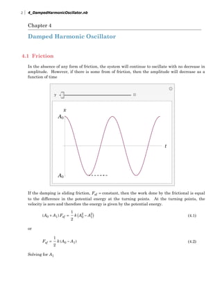
Damped Harmonic Oscillator
4.1 Friction
In the absence of any form of friction, the system will continue to oscillate with no decrease in
amplitude. However, if there is some from of friction, then the amplitude will decrease as a
function of time
g
t
A0
A0
x
If the damping is sliding friction, Fsf = constant, then the work done by the frictional is equal
to the difference in the potential energy at the turning points. At the turning points, the
velocity is zero and therefore the energy is given by the potential energy.
(4.1)HA0 + A1L Fsf =
1
2
k IA0
2
- A1
2
M
or
(4.2)Fsf =
1
2
k HA0 - A1L
Solving for A1
2 4_DampedHarmonicOscillator.nb
2. (4.3)A1 = A0 -
2 Fsf
k
damping coefficient
2 4 6 8 10
-1.0
-0.5
0.5
1.0
4.2 Velocity Dependent Friction
Another common form of friction is proportional to the velocity of the object. This includes, air
drag (at low velocities), viscous drag and magnetic drag.
Formally, the frictional force points in the opposite direction to the velocity
(4.4)Ff = -b v
4_DampedHarmonicOscillator.nb 3
3. t
1
The total force on the mass is then F = -k x - b v. Therefore the equation of motion becomes
(4.5)F = m
d2 x
d t2
= -k x - b
d x
d t
or
(4.6)m
d2 x
d t2
+ b
d x
d t
+ k x = 0
Let’s try our previous trick to find the energy. Multiply the equation by v and rewrite
d2 x
d t2
=
d v
d t
(4.7)m v
d v
d t
+ b v2
+ k v x = 0
or
(4.8)m v
d v
d t
+ k x
d x
d t
= -b v2
The quantity on the left hand side is just the time rate of change of the energy
(4.9)
d
m v2
2
+
k x2
2
d t
=
d E
d t
= -b v2
Previously we had b = 0 and consequently the energy was a constant in time. Now we see that
4 4_DampedHarmonicOscillator.nb
4. d E
d t
< 0 i.e. the energy decreases with time. To estimate the rate of the decrease of E, we can
rewrite the above equation as
(4.10)
d E
d t
= -
2 b
m
1
2
m v2
and replace both sides of the equation by the average value of the quanties. This is not pre-
cisely correct as we are neglecting some terms.
(4.11)
d E
d t
= -
2 b
m
m v2
2
= -
2 b
m
E
2
= -
b
m
E
where we have used the fact that for the undamped harmonic oscillator
1
2
m v2 =
E
2
. Now we
can solve the equation
(4.12)E = E0 ‰
-
b t
m = E0 ‰-t g
= E0 ‰
-
t
t
The average energy decreases exponentially with a characteristic time t = 1 ê g where g = b ê m.
From this equation, we see that the energy will fall by 1 ê ‰ of its initial value in time t
g
1êg
t
E0
‰
E0
x
For an undamped harmonic oscillator,
1
2
k x2 =
E
2
. Therefor one would expect that
4_DampedHarmonicOscillator.nb 5
5. (4.13)x ∂ E ∂ ‰
-
1
2
g t
4.3 Formal Solution
Dividing Equation 4.6 by m, we have that
(4.14)
d2 x
d t2
+
b
m
d x
d t
+
k
m
x =
d2 x
d t2
+ g
d x
d t
+ w0
2 x = 0
Substitute a solution of the form A ‰Â w t
(4.15)
-A ‰Â t w
w2
+  A ‰Â t w
g w + w0
2
A ‰Â t w
= 0
A ‰Â t w I g w - w2 + w0
2M = 0
Because ‰Â w t ∫ 0 or A ∫ 0, A ‰Â w t will be a solution if
(4.16)-Â g w + w2 - w0
2 = 0
or
(4.17)
w1 =
1
2
 g + -g2
+ 4 w0
2
w2 =
1
2
 g - -g2
+ 4 w0
2
The complete solution then is
(4.18)
x@tD = A1 ‰Â t w1 + A2 ‰Â t w2
= A1 ‰
-
t g
2
+
1
2
 t -g2+4 w
0
2
+ A2 ‰
-
t g
2
-
1
2
 t -g2+4 w
0
2
4.3.1 No Damping g = 0
For b = 0, we obtain our previous solution
(4.19)x@tD = A1 ‰Â t w0 + A2 ‰- t w0
For intial condition at t = 0, x@0D = x0 and v@0D = v0, we have that
6 4_DampedHarmonicOscillator.nb
6. (4.20)
x@0D = A1 + A2 = x0
v@0D = Â A1 w0 - Â A2 w0 = v0
Solving for A1 and A2, we obtain
(4.21)
A1 =
x0
2
-
 v0
2 w0
A2 =
x0
2
+
 v0
2 w0
Clearly A1 is the complex conjugate of A2. Rewritting them in exponential form
(4.22)
A1 =
v0
2 + x0
2 w0
2
2 w0
‰-Â f
=
1
2
x0
2
+
v0
2
w0
2
‰-Â f
A2 =
v0
2 + x0
2 w0
2
2 w0
‰Â f
=
1
2
x0
2
+
v0
2
w0
2
‰Â f
where Tan@fD =
v0
x0 w0
The displacement then becomes
(4.23)
x@tD = A1 ‰Â t w0 + A2 ‰- t w0 =
v0
2 + x0
2 w0
2
2 w0
‰Â f- t w0 + ‰- f+ t w0
=
Cos@f - t w0D v0
2 + x0
2 w0
2
w0
4.3.2 Small Damping
g
2
< w0
For
g
2
< w0, the term in the exponent, 4 w0
2
- g2
will be real. Defining a new frequency,
wD =
1
2
4 w0
2
- g2
= w0
2
-
g2
4
, we obtain
4_DampedHarmonicOscillator.nb 7
7. (4.24)
x@tD = A1 ‰-
t g
2
+
1
2
 t -g2
+4 w0
2
+ A2 ‰-
t g
2
-
1
2
 t -g2
+4 w0
2
= ‰-
t g
2 IA1 ‰Â t wD
+ A2 ‰-Â t wD
M
We can now identify wD as the frequency of oscillations of the damped harmonic oscillator. As
before we can rewrite the exponentials in terms of Cosine function with an arbitrary phase.
(4.25)x@tD = A ‰
-
t g
2 Cos@wD t - fD
For intial condition at t = 0, x@0D = x0 and v@0D = v0, we have that
(4.26)
x@0D = A Cos@fD = x0
v@0D = -
1
2
A g Cos@fD + A Sin@fD wD = v0
Substituting, for Cos[f] from the first equation into the second, we have that
(4.27)-
g x0
2
+ A Sin@fD wD = v0
Therefore
(4.28)
A Cos@fD = x0
A Sin@fD =
2 v0 + g x0
2 wD
Solving for A and f
(4.29)
A = x0
2
+
H2 v0 + g x0L2
4 wD
2
Tan@fD =
2 v0 + g x0
2 x0 wD
One can check this answer by taking the limit as g Ø 0 (no damping), wD Ø w0 and the expres-
sions for A and f should reduce to our previous result.
(4.30)
A = x0
2 +
v0
2
w0
2
Tan@fD =
v0
x0 w0
8 4_DampedHarmonicOscillator.nb
8. g
2
w
7.5 3.5
q0 q
°
0
1.22 0
2 4 6 8 10
-1.0
-0.5
0.5
1.0
initial angle HradiansL
initial angular velocity
4.3.3 Critical Damping
g
2
= w0
At
g
2
= w0, the frequency wD vanishes and the expression in the exponent reduces to
(4.31)-
g
2
≤
1
2
 -g2
+ 4 w0
2
Ø -
g
2
The solution no longer has an oscillatory part. In addition one no longer has two solutions
that can be used to fit arbitrary initial conditions.
The general solution as a function of time becomes
(4.32)x@tD = ‰
-
t g
2 HA + B tL
The second term is necessary to satisfy all possible initial conditions. Differentiating
(4.33)
v@tD = -
1
2
‰
-
t g
2 HA g + B H-2 + t gLL
a@tD =
1
4
‰
-
t g
2 g HA g + B H-4 + t gLL
4_DampedHarmonicOscillator.nb 9
9. Substituting in the differential equation
(4.34)
d2 x
d t2
+ g
d x
d t
+ w0
2
x = 0
1
4
‰
-
t g
2 g HA g + B H-4 + t gLL + -
1
2
‰
-
t g
2 g HA g + B H-2 + t gLL + w0
2
‰
-
t g
2 HA + B t
-
1
4
‰
-
t g
2 HA + B tL Ig2 - 4 w0
2M = 0
which by the definition, g2 = 4 w0
2, is identically equal to zero
To determine A and B from the initial conditions, equate
(4.35)
x@0D = ‰
-
t g
2 HA + B tL
t=0
= A
v@tD = -
1
2
‰
-
t g
2 HA g + B H-2 + t gLL
t=0
=
1
2
H2 B - A gL
Solving for A and B
(4.36)
A = x0
B =
1
2
H2 v0 + g x0L
and therefore the general solution becomes
(4.37)x@tD = ‰
-
t g
2 x0 +
1
2
t H2 v0 + g x0L
4.3.4 Overdamping
g
2
> w0
For
g
2
> w0, the argument of the square root becomes negative. Taking the -1 out of the
squareroot so that its argument is now positive, the frequency, w, becomes completely
imaginary
(4.38)
w1 =
 g
2
+ -
g2
4
+ w0
2 ->
 g
2
+ Â
g2
4
- w0
2
w1 =
 g
2
- -
g2
4
+ w0
2
->
 g
2
- Â
g2
4
- w0
2
10 4_DampedHarmonicOscillator.nb
10. Again, there are no oscillatory terms. Both solutions are dying exponentials
(4.39)
x@tD = A1 ‰
t -
g
2
-
g2
4
-w
0
2
+ A2 ‰
t -
g
2
+
g2
4
-w
0
2
Although the second term contains a growing exponential,
gD
2
= J
g
2
N
2
- w0
2 <
g
2
and so the
overal function is still a dying exponential.
As before, to determine A1 and A2 from the initial conditions, equate
(4.40)x@0D = ‰
t J-
g
2
-
gD
2
N
A1 + ‰
t J-
g
2
+
gD
2
N
A2
t=0
= A1 + A2
and
(4.41)
v@0D =
1
2
‰
-
1
2
t Ig+gDM
I‰t gD A2 H-g + gDL - A1 Hg + gDLM
t=0
=
1
2
HA2 H-g + gDL - A1 Hg + gDLL
Solving for A1 and A2
(4.42)
A1 =
-2 v0 + x0 H-g + gDL
2 gD
A2 =
2 v0 + x0 Hg + gDL
2 gD
and therefore the general solution becomes
(4.43)x@tD =
1
2 gD
‰
-
1
2
t Ig+gDM
I2 I-1 + ‰t gDM v0 + x0 I-g + gD + ‰t gD Hg + gDLMM
Note that this solution looks very much like our original solution for the underdamping case.
In particular if we let g2 - 4 w0
2 Ø Â 4 w0
2 - g2 = 2 Â wD, then the above solution becomes
(4.44)x@tD =
1
2 Â wD
‰
-
1
2
Ht gL
CoshB
2
2
t  wDF 2  wD x0 + SinhB
1
2
t 2 Â wDF H2 v0 + g x0L
Now, Cosh@Â yD =
‰Â y + ‰- y
2
= Cos@yD and Sinh@Â yD =
‰Â y - ‰- y
2
= Â Sin@yD so that the above
expression reduces to
4_DampedHarmonicOscillator.nb 11
11. x@tD = -
 ‰
-
t g
2 HÂ Sin@t wDD H2 v0 + g x0L + 2 Â Cos@t wDD x0 wDL
2 wD
= ‰
-
t g
2 Cos@t wDD x0 +
Sin@t wDD Jv0 +
g x0
2
N
wD
Equating x0 = Cos@fD and
v0 +
g
2
x0
wD
= Sin@fD, then the above solution becomes the solution for
an underdamped harmonic oscillator
(4.46)x@tD = Cos@f + t wDD x0
2
+
Jv0 +
g x0
2
N
2
wD
2
4.4 Quality Factor or Q
A dimensionless quantity used to measure the amount of damping is given by for a harmonic
oscillator is defined as
(4.47)Q = H2 pHaverage energy storedLL ê Henergy lost per cycleL
As defined the Q will be large if the damping is small. We know that the average energy is
given approximately by E@tD º E0 ‰-g tê2. The change is the energy in one period t is therefore
(4.48)DE = E@t0D - E@t + t0D = ‰-g t0 H1 - ‰-g t
L E0
For small damping g t << 1, one can expand the exponential, ‰-g t º 1 - g t + ... so that
(4.49)DE = ‰-g t0 g t E0
Substituting this into the expression for the Q
(4.50)Q =
2 ‰-g t0 p E0
‰-g t0 g t E0
=
2 p
g t
=
w
g
where we have used the fact that w =
2 p
t
. The following illustrates the behavior for several
values of the Q.
12 4_DampedHarmonicOscillator.nb
12. 4 6 8 10
= 0.0125664 Q = 500
0 2 4 6 8 10
-1.0
-0.5
0.0
0.5
1.0 g = 0.0314159 Q = 200
0 2 4 6
-1.0
-0.5
0.0
0.5
1.0 g = 0.0628319 Q =
4 6 8 10
g = 0.125664 Q = 50
0 2 4 6 8 10
-1.0
-0.5
0.0
0.5
1.0 g = 0.314159 Q = 20
0 2 4 6
-1.0
-0.5
0.0
0.5
1.0 g = 0.628319 Q =
4 6 8 10
g = 1.25664 Q = 5
0 2 4 6 8 10
-1.0
-0.5
0.0
0.5
1.0 g = 3.14159 Q = 2
0 2 4 6
-1.0
-0.5
0.0
0.5
1.0 g = 6.28319 Q =
4 6 8 10
g = 12.5664 Q = 0.5
0 2 4 6 8 10
-1.0
-0.5
0.0
0.5
1.0 g = 31.4159 Q = 0.2
0 2 4 6
-1.0
-0.5
0.0
0.5
1.0 g = 62.8319 Q =
4.5 Energy of Damped Harmonic Oscillator
Using the expression for an underdamped harmonic oscillator, x@tD = A Cos@wD t + fD e-g tê2, the
potential energy becomes
(4.51)PE =
1
2
k x@tD2
=
1
2
m w2
x@tD2
=
1
2
A2
‰-t g
m w2
Cos@f + t wDD2
To calculate the kinetic energy, first calculate the velocity
4_DampedHarmonicOscillator.nb 13
13. (4.52)v@tD = -
1
2
A ‰
-
t g
2 g Cos@f + t wDD - A ‰
-
t g
2 Sin@f + t wDD wD
and the kinetic energy becomes
(4.53)
PE =
1
2
m v@tD2
=
1
2
m -
1
2
A ‰
-
t g
2 g Cos@f + t wDD - A ‰
-
t g
2 Sin@f + t wDD wD
2
=
1
8
A2
‰-t g
k Hg Cos@f + t wDD + 2 Sin@f + t wDD wDL2
The total energy is then
(4.54)
E@tD =
1
8
A2
‰-t g
m
IIg2
+ 4 w2
M Cos@f + t wDD2
+ 2 g Sin@2 Hf + t wDLD wD + 4 Sin@f + t wDD2
wD
2
M
Substituting w2 =
g2
4
+ wD
2
(4.55)
E@tD =
1
4
A2
‰-t g
m Ig2
Cos@f + t wDD2
+ g Sin@2 Hf + t wDLD wD + 2 wD
2
M
E@tD =
1
2
A2
‰-t g
m wD
2
1 +
g2 Cos@f + t wDD2
2 wD
2
+
g Sin@2 Hf + t wDLD
2 wD
Plotting the total energies assuming f = 0.
14 4_DampedHarmonicOscillator.nb
14. tmax
g
w
0.0 0.2 0.4 0.6 0.8 1.0
0.0
0.2
0.4
0.6
0.8
1.0
1.2
............................................................
4_DampedHarmonicOscillator.nb 15