The document summarizes four numerical methods commonly used in geomechanics: 1. The Distinct Element Method (DEM) explicitly models discontinuities. 2. The Discontinuous Deformation Analysis Method (DDA) can consider discontinuities explicitly or implicitly. 3. The Bonded Particle Method (BPM) models geomaterials as an assembly of discrete particles. 4. The Artificial Neural Network Method (ANN) is a data-driven modeling approach not classified as continuum or discontinuum. The document provides a brief overview of the fundamental algorithms of each method and examples of their applications.

1. Antonio Bobet
NUMERICAL METHODS IN GEOMECHANICS
Antonio Bobet
School of Civil Engineering, Purdue University, West Lafayette, IN, USA
:‫اﻟﺨﻼﺻـﺔ‬
‫ﺗﻘﺪم هﺬﻩ اﻟﻮرﻗﺔ وﺻﻔﺎ ﻟﻠﻄﺮق اﻟﻌﺪدﻳﺔ اﻷآﺜﺮ اﺳﺘﺨﺪاﻣﺎ ﻓﻲ اﻟﻤﻴﻜﺎﻧﻴﻜﺎ اﻟﺠﻴﻮﻟﻮﺟﻴﺔ. وهﻲ أرﺑﻌﺔ ﻃﺮق : )1( ﻃﺮﻳﻘﺔ اﻟﻌﻨﺼﺮ اﻟﻤﻤﻴﺰ )2( ﻃﺮﻳﻘﺔ ﺗﺤﻠﻴﻞ‬
ً
.‫اﻟﻨﺸﻮة اﻟﻤﺘﻘﻄﻊ )3( ﻃﺮﻳﻘﺔ اﻟﺘﺤﺎم اﻟﺠﺴﻴﻤﺎت )4( ﻃﺮﻳﻘﺔ اﻟﺸﺒﻜﺔ اﻟﻌﺼﺒﻴﺔ اﻟﺼﻨﺎﻋﻴﺔ‬
.‫وﺗﻀﻤﻨﺖ اﻟﻮرﻗﺔ أﻳﻀﺎ وﺻﻔﺎ ﻣﻮﺟﺰا ﻟﺘﻄﺒﻴﻖ اﻟﻤﺒﺎدئ اﻟﺨﻮارزﻣﻴﺔ ﻟﻜﻞ ﻃﺮﻳﻘﺔ إﺿﺎﻓﺔ إﻟﻰ ﺣﺎﻟﺔ ﺑﺴﻴﻄﺔ ﻟﺘﻮﺿﻴﺢ اﺳﺘﺨﺪاﻣﻬﺎ‬
ً ً ً
______________________
*Corresponding Author:
E-mail: bobet@purdue.edu
Paper Received November 7, 2009; Paper Revised January 17, 2009; Paper Accepted February 3, 2010
April 2010 The Arabian Journal for Science and Engineering, Volume 35, Number 1B 27

2. Antonio Bobet
ABSTRACT
The paper presents a description of the numerical methods most used in geomechanics. The following methods
are included: (1) The Distinct Element Method; (2) The Discontinuous Deformation Analysis Method; (3) The
Bonded Particle Method; and (4) The Artificial Neural Network Method. A brief description of the fundamental
algorithms that apply to each method is included, as well as a simple case to illustrate their use.
Key words: numerical methods, geomechanics, continuum, discontinuum, finite difference, finite element, discrete
element, discontinuous deformation analysis, bonded particle, artificial neural network
28 The Arabian Journal for Science and Engineering, Volume 35, Number 1B April 2010

3. Antonio Bobet
NUMERICAL METHODS IN GEOMECHANICS
1. INTRODUCTION
Analytical methods are very useful in geomechanics because they provide results with very limited effort and
highlight the most important variables that determine the solution of a problem. Analytical solutions, however, have
often a limited application since they must be used within the range of assumptions made for their development.
Such assumptions usually include elastic behavior, homogeneous, isotropic material, time independent behavior,
quasi-static loading, etc. Geomaterials such as soils and rock masses display non-linear behavior, either because this
is inherent to the material or because it has been externally induced (e.g., past stress history). Rocks and soils may
not be isotropic or homogeneous, and the loading may not be static, or the geometry of the problem may be complex.
In these cases, solutions can only be obtained numerically.
Numerical methods give only approximations to the correct or exact mathematical solution. This is so because
some simplifications are made to solve the system of differential equations either inside the continuum or at the
boundaries of the discretization. It has to be mentioned also that the problem that is solved is the conceptualization
that is done of the actual physical problem. The conceptualization applies to the geometry of the problem, the
loading process or history, and the response of the geomaterials to loading. The better the approximation to the field
problem through this conceptualization process, the more accurate the solution will be with respect to the response
observed in the field.
Numerical methods have been extensively used in the past several decades due to advances in computing power.
In a broad sense, numerical methods can be classified into continuum and discontinuum methods [1,2]. Continuum
methods may incorporate the discontinuities in the medium, if present, explicit or implicitly, while in discontinuum
methods, discontinuities are incorporated explicitly. The need to use, for a particular problem, continuum or
discontinuum methods depends on the size, or scale, of the discontinuities with respect to the size, or scale, of the
problem that needs to be solved. There are no quantitative guidelines to determine when one method should be used
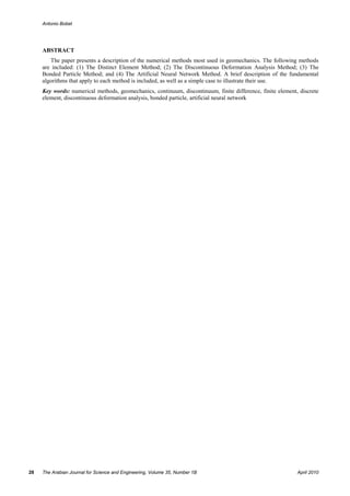
instead of the other one. Figure 1 (following Brady [3]) provides some qualitative guidance. For example, Figure
1(a) illustrates an opening in a medium without discontinuities; in this case the displacement field is continuous and
thus continuum numerical methods are appropriate. Figure 1(b) shows a tunnel excavated in a medium with a small
number of discontinuities which divide the medium into a small number of continuous regions. The displacement
field will be continuous inside each region but may be discontinuous across the discontinuities. If a continuum model
is used, the model should be able to consider the specific discontinuities. The medium depicted in Figure 1(c) is
determined by a number of discontinuities with spacing and continuity such that the blocks defined are within the
scale of the opening. In this case, displacements may be determined by the slip along the discontinuities and rotation
of the blocks. Thus, a discontinuum numerical method seems appropriate. If the medium is heavily jointed such that
the blocks defined by the discontinuities have a size much smaller than the opening, e.g., Figure 1(d), a pseudo-
continuous displacement field is produced and the use of a continuum model seems reasonable.
There is quite a large number of numerical methods that have been used in the literature to estimate the behavior
of geomaterials. The most important, or at least the most used methods are: Continuum, Finite Difference Method
(FDM), Finite Element Method (FEM) and Boundary Element Method (BEM); Discontinuum, Distinct Element
Method (DEM), Discontinuous Deformation Analysis (DDA), and Bonded Particle Model (BPM). There are two
other methods which do not follow this classification: Meshless Methods (MM) and Artificial Neural Networks
(ANN). While all methods are relevant, the paper focuses on DEM, DDA, BPM, and ANN, which have recently
seen a significant use growth. The following sections provide the fundamental assumptions and the mathematical
framework for each method and an overview of the range of problems where each method has been successfully
used. A brief description of continuum methods is also included.
2. CONTINUUM METHODS: FINITE DIFFERENCE METHOD, FINITE ELEMENT METHOD, AND
BOUNDARY ELEMENT METHOD
The Finite Element Method (FEM), the Finite Difference Method (FDM), and the Boundary Element Method
(BEM) are the continuum methods most used in geomechanics [4,5]. In these methods, either the medium and the
boundaries (FEM and FDM) or only the boundaries (BEM) are discretized.
The Finite Difference Method (FDM) is based on the premise that governing differential equations can be
adequately represented by finite differences. The method is the oldest among the numerical methods in
geomechanics and was used even before the arrival of computers. Timoshenko and Goodier [6] attribute the first
application of the method to Runge, who in 1908 used it for the solution of torsion problems. With the FDM, the set
of differential equations is reduced to a system of linear equations, which can be solved by any of the classical
methods. Southwell [7] developed the relaxation method, which provides a fast solution of the system of equations;
this promoted a much wider use of the FDM. The method really took off with the advent of computers.
April 2010 The Arabian Journal for Science and Engineering, Volume 35, Number 1B 29

4. Antonio Bobet
Figure 1. Continuum and Discrete Models
With the method a grid is superimposed to the domain, as shown in Figure 2. In the figure, the sub-indices
represent the position of the point in the grid; for example, i,j represents a point with coordinates (xi, xj), i+1,j the
point (xi+h, xj), i,j+1 the point (xi, xj+k), and so on. The method relies on the approximation of the field equations,
i.e. equilibrium, strain compatibility, etc. by finite difference formulas. Discontinuities can be incorporated in the
model by using grid points on each side of the discontinuity. The relative displacement between corresponding grid
points determines the slip along the discontinuity, and frictional laws (e.g., Coulomb) can be enforced by adding new
equations to the system of equations that relate shear stress with normal stress. Normal and shear displacements can
also be related to the shear and normal stiffness of the discontinuity.
Figure 2. Finite Difference Grid in 2D
30 The Arabian Journal for Science and Engineering, Volume 35, Number 1B April 2010

5. Antonio Bobet
The method can also be readily used to solve dynamic problems, where displacements are a function of position
and time. Explicit time integration techniques are often used to provide solutions using small time increment steps.
Dynamic problems require a maximum time step to ensure stability of the solution, which is given by
⎛∆ x⎞
∆t = min ⎜ ⎟
⎜ Cp ⎟
⎝ ⎠ (1)
K+4/3 G
Cp =
ρ
Cp is the compressional or P-wave velocity in the medium, ∆x is the grid spacings, K is the bulk modulus, G the
shear modulus, and ρ the density of the medium. Equation (1) indicates that the maximum time step is controlled by
the stiffer material in the medium. It is not unusual to run tens of thousands of steps to complete a numerical
analysis. While the number of steps is quite large, the time required to complete each step and the memory required
to store the solution is small, and, thus, complex dynamic problems can be analyzed in a reasonable period of time.
The finite difference approach is very well-suited to incorporate non-linear behavior. The solution is then
obtained on a stepwise process involving sufficiently small loading increments until the desired final state is reached.
At the end of each loading step, displacements at the grid points are obtained; stresses are then updated based on the
non-linear behavior of the material, and another small loading increment is added. The new increment starts with the
updated stress field from the previous increment. This is a forward scheme that does not require iteration, unlike
other techniques such as Finite Element Methods that use implicit solution methods.
The Finite Element Method (FEM) is by far the method used the most for the analysis of continuous or quasi-
continuous media. The term “Finite Element”, according to Bathe [8], was first introduced by Clough [9]. The
method consists of discretization of the continuum into small elements that intersect at their nodes (Figure 3). The
method relies on the assumption that, through appropriately chosen interpolation functions, displacements at any
point within the element can be accurately obtained from the displacements of the nodes. The method is based on the
principle of virtual displacements, which states that, for a body in equilibrium, any compatible (i.e., satisfies
boundary conditions) small virtual displacements applied to the body, the total internal work associated with the
virtual displacement field must be equal to the total virtual external work.
Figure 3. Finite Element Discretization in 2D
With the Boundary Element Method (BEM), only the boundaries of the continuum need to be discretized. See
Figure 4. This is in contrast to the other two continuum methods, the Finite Difference and the Finite Element
methods, where the entire medium has to be discretized. Also, if the medium extends to infinity, which is common in
problems in geomechanics, no artificial boundaries such as those needed in FDM and FEM are required. The BEM
automatically satisfies far-field conditions. In the BEM, the solution is approximated at the boundaries while
equilibrium and compatibility are exactly satisfied in the interior of the medium. In FDM and FEM, the
approximations are made inside the medium. The advantage of limiting the discretization to the boundaries is that
the problem is reduced by one order: from 3D to a 2D surface problem at the boundary, and from 2D to a line
problem. Thus the method is very attractive for those problems where the volume to boundary surface ratio is large.
April 2010 The Arabian Journal for Science and Engineering, Volume 35, Number 1B 31

6. Antonio Bobet
Figure 4. Example of Discretization with Boundary Elements in 2D
The technique used in BEM consists in essence of transforming the governing differential equations, which apply
to the entire medium, to integral equations which only consider boundary values [10–12]. In a boundary value
problem, some parameters such as stresses and displacements are known while others are not, which then are part of
the solution. There are two approaches to solve for the unknown parameters. In the first approach (Direct BEM), the
unknowns are solved directly, and once they are obtained, stresses and displacements at any point in the continuum
can be obtained directly from the solution. In the second approach (Indirect BEM), the solution is found in terms of
some “fictitious” quantities, typically stresses or displacements. The fictitious quantities are obtained first and the
stresses and displacements at any point in the medium are expressed in terms of these fictitious quantities.
Boundary Element Methods are particularly well-suited to address static continuum problems with small
boundary to volume ratios, with elastic behavior, and with stresses or displacements applied to the boundaries.
Actual problems may not always conform to these limitations. For example, rocks and soil deposits may undergo
significant yielding under moderate stresses, gravity forces may be significant for shallow geostructures, and inertia
may play an important role with dynamic loading (e.g., blasting, earthquake). Dynamic and body forces require
integration over the entire volume domain which leads to the need for discretization of the entire continuum. The
plasticity algorithms require integration at least over the volume of the material that undergoes yielding and
convergence of the solution, as with FEM, is attained through iteration. With plastic deformations and with cases
where integration needs to be extended over part or the entire volume, the advantage that the BEM offers regarding
limited discretization of the continuum may be lost. Efficient hybrid BEM-FEM solutions are possible, where a FEM
discretization is used for those parts of the continuum where plastic deformations occur, while Boundary Elements
are used in elastic regions. The advantage of the coupled FEM-BEM is reduced discretization and automatic
satisfaction of boundary conditions at infinity. The challenge of the hybrid approach is the generation of nodal forces
and displacements from the BEM that are consistent with those of FEM, and that the resulting stiffness matrix is
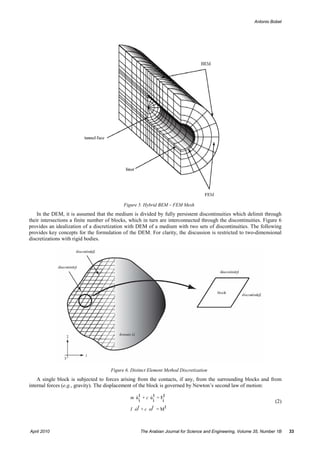
non-symmetric (in contrast with FEM where the stiffness matrix is generally symmetric). Figure 5 shows an example
of a hybrid discretization of a tunnel, where the tunnel liner and a volume of the ground next to the tunnel where
plastic deformations occur, are discretized with Finite Elements. Far from the tunnel and where the deformations are
elastic, Boundary Elements are used.
3. DISCONTINUUM: THE DISTINCT ELEMENT METHOD
The Distinct Element Method (DEM) was introduced by Cundall [13] as a model to simulate large movements in
blocky rock masses, and then used for soils which were modeled as discs [14]. Later on, the method has been applied
to spherical and polyhedral blocks [4,15–19] for both soils and rocks.
The DEM belongs to the family of Discrete Element Methods, which Cundall and Hart [18] define as those that:
(1) allow finite displacements and rotations of discrete bodies, including detachment; and (2) automatically
recognize new contacts between bodies during calculations. Discrete Element Methods need to address three key
issues: (1) representation of contacts; (2) representation of solid material; and (3) detection and revision of contacts
during execution. An in-depth discussion of these issues is provided by Cundall and Hart [18].
32 The Arabian Journal for Science and Engineering, Volume 35, Number 1B April 2010

7. Antonio Bobet
Figure 5. Hybrid BEM – FEM Mesh
In the DEM, it is assumed that the medium is divided by fully persistent discontinuities which delimit through
their intersections a finite number of blocks, which in turn are interconnected through the discontinuities. Figure 6
provides an idealization of a discretization with DEM of a medium with two sets of discontinuities. The following
provides key concepts for the formulation of the DEM. For clarity, the discussion is restricted to two-dimensional
discretizations with rigid bodies.
Figure 6. Distinct Element Method Discretization
A single block is subjected to forces arising from the contacts, if any, from the surrounding blocks and from
internal forces (e.g., gravity). The displacement of the block is governed by Newton’s second law of motion:
m u t + c u t = Ft
i i i (2)
I ωt + c ωt = M t
April 2010 The Arabian Journal for Science and Engineering, Volume 35, Number 1B 33

8. Antonio Bobet
where t is time, m is the mass, I is the moment of inertia of the element, ui is the displacement of the gravity center of
the element in the direction i, u i and ui are the acceleration and the velocity of the gravity center, ω and ω are the
angular rotation and angular velocity of the element, c is the viscous damping, and Fi and M are the resultant force
and moment applied at the center of gravity. In the DEM Equation (2) is solved in the time domain using an explicit
finite difference method. Using the central finite difference, approximation velocities and displacements are given by
⎡ t ⎤
t +∆t / 2 = ⎢ D u t −∆t / 2 + Fi ∆t ⎥ D
u
i ⎢ 1 i m ⎥ 2
⎢
⎣ ⎥
⎦
⎡ t ⎤
ωt +∆t / 2 = ⎢ D1 ωt −∆t / 2 +
M
∆t ⎥ D 2
⎢ m ⎥
⎣ ⎦
c ∆t (3)
D1 = 1-
m 2
1
D2 =
c ∆t
1+
m 2
ut +∆t = ut +u t +∆t / 2 ∆t
i i i
θ t +∆t = θ t +ωt +∆t / 2 ∆t
The forces acting at the boundaries are originated by the interaction of the element with the surrounding
elements. At each boundary, a normal and a shear force appear as the result of the relative movements between the
two elements that share the discontinuity. The forces at the interface may be obtained using a penalty method where
the magnitude of the forces is related to the relative movements between the two elements and the stiffness of the
discontinuity. Figure 7(a) shows the positive forces at the top of the element, and Figure 7(b) shows an idealization
of the contact between blocks. The normal force is proportional to the relative movement of the two blocks across
the contact and along the normal direction. The shear force is proportional to the relative movement along the
direction of the contact. Expressions for the forces are
Fn +∆t = Fn - K n ∆u ∆t Ac - β K n ∆u ∆t Ac
t t
n n (4)
Fs +∆t = Fs - Ks ∆u s t Ac - β Ks ∆u s t Ac
t t ∆ ∆
Kn and Ks are the normal and shear stiffness of the contact (subscripts n and s refer to the directions normal and
parallel to the discontinuity, respectively); ∆un and ∆us are relative displacements between the two elements, and Ac
is the contact area. A damping factor, the third term on the right-hand side of the equation, is normally included to
attenuate or prevent “rattling” of the contact between blocks. Damping (Cn and Cs in Figure 7) is often expressed as
proportional to the normal and shear stiffness (βKn and βKs in (4)), but other expressions for damping have been
proposed (e.g., damping proportional to the rate of change of the kinetic energy of the element [15]).
Figure 7. Forces at the Boundary of DEM Elements
34 The Arabian Journal for Science and Engineering, Volume 35, Number 1B April 2010

9. Antonio Bobet
The magnitude of the shear force is limited by the constitutive relation used for the contact surface. For a
Coulomb-type friction law,
Fs +∆t ≤ c Ac + Fn +∆t tan φ
t t (5)
where c and φ are the cohesion and friction angles of the contact surface. If the shear force obtained from (4) is
larger that that from (5), it is reduced to the limiting magnitude given by (5).
The calculations are performed from one state, where the solution is fully known, to another state in small time
increments. The procedure is as follows [17]: The law of motion is applied through Equation (3) with current forces
to update the position of each element. As a result, the relative displacements and velocities at the contacts between
elements are obtained. From the relative displacements, contact forces are updated using Equation (4) and new
resultant forces and moments at the center of gravity of each element are computed. The cycle is repeated with small
increments until the final solution is obtained. In the formulation, time can represent actual time when performing a
dynamic analysis, or a fictitious parameter to represent loading increment from one loading stage to the next.
As with the Finite Difference Method, numerical stability requires a time increment smaller than the critical time
step, which is given by [17]:
mmin
∆tcrit = κ (6)
2 K max
where mmin is the smallest element mass, Kmax is the largest normal or shear stiffness in the discretization, and κ is a
factor that takes into account the fact that an element may be in contact with more than one element. A value for κ
equal to 0.1 has been suggested [17].
Typical runs are completed with thousands of cycles involving very small time increments. The solution of
equations (3) and (4) is a forward process, and, thus, the computer time required in each cycle is very small; also, the
storage information needed for each element is small. Therefore, the process discussed so far does not require
intensive computation power or large storage capabilities. Where such requirements become significant is for the
algorithm to recognize and keep track of all the contacts between elements during execution. A very simple
procedure would be to compare the position of each element with the rest of the elements at the end of each cycle.
For a discretization with n elements, this would require of the order of n2 operations in each cycle, which would
make the entire method impractical. Considerable effort has been done to develop efficient algorithms, which on the
one hand need to accurately describe the interaction between elements, and on the other hand are not
computationally intensive. The problem is complex as the algorithms need to identify not only what elements are in
contact but also the type of contact: corner to corner, corner to edge, or edge to edge, since the magnitude and
direction of the contact forces depend on the type of contact. A number of approaches has been proposed to identify
contacts, such as global searching algorithms, buffer zone definition, contact or field zone, binary tree structures,
space decomposition and alternating digital tree [16,20–23]. A comprehensive review of these methods is provided
in [24].
The Distinct Element Method is nowadays a very versatile and extensively validated procedure. It has been
developed for full three-dimensional problems, and by discretizing the elements with Finite Difference or Finite
Element meshes, can be applied to deformable bodies [4,18,25] and to fragmentation of discontinua [20, 25]. It can
be used for static and for dynamic calculations [26,27]. Heuze and Morris [28] provide an extensive overview of the
DEM as applied to jointed rock masses. One fundamental advantage of the DEM is that pre-existing joints in rock
can be incorporated into a DEM model directly, and the joints are allowed to undergo large deformations. Detailed
joint constitutive models (see [29] for a review) can also be used to combine experimentally observed fracture
properties (such as joint dilation, friction angle, and cohesion) with the DEM approach.
Figure 8(a) shows the discretization used to investigate the response of a tunnel in a discontinuous rock mass
subjected to blast loading [30,31]. Figures 8(b) and (c) show the response of the tunnel immediately after detonation
and 30 ms later. The simulations were run using parallel processing and the Livermore Distinct Element Code
(LDEC), and consisted of 8 million blocks with approximately 100 million contacts, with typical block size of 30
cm, making these the largest simulations of this type performed to date.
April 2010 The Arabian Journal for Science and Engineering, Volume 35, Number 1B 35

10. Antonio Bobet
Figure 8. DEM simulation of an underground structure subjected to dynamic loading (Morris and Block, 2006)
4. DISCONTINUUM: DISCONTINUOUS DEFORMATION ANALYSIS
The Discontinuous Deformation Analysis (DDA) is a Discrete Element Method following the definition by
Cundall and Hart [18], as outlined in the preceding section. The method started with the work of Shi and Goodman
[32,33], and since then it has received considerable attention by the geoengineering community.
The method is fully described in [34,35]. In essence, the medium is discretized into elements or blocks which are
in contact with each other only through the discontinuities. The discretization used in Figure 6 to illustrate the DEM
could perfectly apply to the DDA. There are fundamental differences between the DEM and DDA. In the DEM each
block is treated separately, while in the DDA, the total potential energy of the system is minimized to find the
solution. In the DEM, stresses and forces are unknowns while displacements are computed from stresses; in DDA
the displacements are the unknowns. In the DEM, the contacts are resolved using a penalty method which results in
the definition of the contact forces, while in the DDA, interpenetration of blocks is prevented by adding springs to
the contacts. The DEM uses an explicit procedure to solve the equilibrium equations and the DDA is an implicit
method. While the DDA is a fully discontinuous analysis, it resembles and follows the procedures developed for
FEM.
The DDA, similar to the DEM, needs to address three key issues: (1) representation of contacts; (2)
representation of solid material; and (3) detection and revision of contacts during execution. The elements can be
convex or non-convex, and their shapes are determined by the location of their contacts with the neighboring
elements. Thus, blocks are represented by polyhedra, with the contacts between blocks consisting of edge to face,
edge to edge, or face to face.
It is assumed that any large displacements or deformations are the result of the accumulation of small
displacements and deformations after a sufficiently large number of steps. Within each step, the displacements of
any block are small and, thus, they can be given, in 2-D, by a first order approximation of the form
u = u o + (x-x o ) a1 +(y-yo ) a 2
(7)
v = vo + (x-x o ) b1 +(y-yo ) b2
where u and v are the x- and y-axis displacements of a point with coordinates x and y; uo and vo are the rigid body
motions at point xo, yo and ai and bi i=1,2 are constants. Strains can be computed from (7). In turn displacements can
be expressed as a function of strains as follows:
36 The Arabian Journal for Science and Engineering, Volume 35, Number 1B April 2010

11. Antonio Bobet
⎛1 ⎞
u = u o + (x-x o ) ε xx +(y-yo ) ⎜ γ xy -ro ⎟
⎝2 ⎠
(8)
⎛ 1 ⎞
v = vo + (y-yo ) ε yy +(x-x o ) ⎜ γ xy +ro ⎟
⎝2 ⎠
where εxx, εyy and γxy are the axial strains and the shear strains in the x and y axis, respectively, and ro is the rigid
block rotation, in radians, about point xo, yo. Equations (8) are expressed in matrix notation
U =TD (9)
where U = (u, v), DT = (uo, vo, ro, εxx, εyy γxy) and T are the appropriate coefficients from (8). The matrix D represents
the unknowns for each element; thus, there are a total of 6 degrees of freedom or unknowns. Note that strains in each
element are constant. For a system of N elements or blocks, the total number of unknowns is 6N. Minimization of
the potential energy of the system of blocks, following FEM convention, is expressed as
K ij D j = Fi (10)
Dj is made of 6x1 sub-matrices that contain the 6 unknowns of each element j; Kij is composed of 6x6 stiffness
sub-matrices associated with the corresponding degrees of freedom of element j, and Fi is a set of 6x1 force sub-
matrices of element i. Kii depends on the material properties of element i and Kij (i≠j) on the contacts between
elements. The sub-matrices Kij are obtained by minimizing the potential energy associated with strain energy, initial
stresses, concentrated and distributed loads, body forces, inertia forces, viscosity, displacement constraints at the
element contacts, etc. Full derivation of the equations are provided in [35].
In the DDA, no tension and no penetration between blocks are allowed. The kinematics of the block system are
incorporated into the equations of equilibrium (10) by adding very stiff springs between appropriate elements to lock
the movement in the corresponding direction. Tension between two elements can be modeled by applying a lock in
the direction where tension is permitted; once the lock is removed (i.e., a critical tensile threshold is reached) the
elements can separate. Hence, by adding or removing locks along appropriate directions, movements between blocks
can be avoided, thus preventing penetration. Within a certain loading step (load increment), an iteration process is
applied where locks are added or removed as appropriate until all kinematic constrains (e.g., no penetration) are
satisfied. To impose the kinematics of the problem requires addressing two issues: (1) determine contacts between
blocks, and (2) add to the global equilibrium equations the appropriate stiff springs.
The contact identification process starts after definition of the elements where some threshold distance is
established such that only elements within the threshold distance are checked for contact. As the simulation
proceeds, potential contacts between elements are updated. If within a single step, the relative displacement between
two elements is smaller than their initial distance, no contact check is performed. If interpenetration between two
elements is detected, then stiff springs are placed between the two elements and the system is recalculated.
The procedure of solving the equilibrium equations, determining interpenetration, and adding stiff springs is
repeated until no interpenetration occurs. At the end of each iteration, the spring force is calculated. If the component
of the force normal to the contact is tensile, the normal spring is removed. If the component of the force parallel to
the contact is larger than the maximum allowed by the constitutive model (e.g., Fs > µFn, Coulomb), a spring normal
to the contact is placed to allow for sliding and prevent penetration in the normal direction; if smaller than the
maximum allowed, springs both in the normal and parallel directions are placed to prevent any relative movement at
the contact.
The method, which was originally developed for 2D problems [32,33,35], has been expanded to 3D [36,37]. The
limitation that the original DDA had that the blocks could not break has been overcome by new developments in
modeling, where blocks are divided into sub-blocks when tensile or shear stresses reach the strength of the material;
thus, the DDA has been extended to fragmentation and fracture propagation problems [38,39]. Validation of the
Displacement Discontinuity Analysis has been done extensively by comparing predictions from the method with
analytical solutions, with other numerical methods, with laboratory and field measurements (e.g., [40–45; an
extensive review can be found in [46]).
Figure 9 illustrates an example application of the DDA method [47]. In the figure, a shallow rectangular tunnel in
a rock mass medium with two joint sets is subjected to a vertical load on the surface. The figure shows the different
stages of the failure, from initial conditions, Figure 9(a), to final failure, Figure 9(f).
April 2010 The Arabian Journal for Science and Engineering, Volume 35, Number 1B 37

12. Antonio Bobet
Figure 9. Example application of DDA Method. 8×5m tunnel with a vertical load applied at the surface. (a) initial geometry; (b)
at time, t=0.001 s; (c) t=0.002s; (d) t=0.003 s; (e) t=0.004 s; and (f) t=0.005 s. Adapted from Jing, (1998).
5. DISCONTINUUM: BONDED PARTICLE METHOD
The Bonded Particle Method [19] originates from the application of the DEM to a discontinuous medium
modeled as discs in two dimensions or spheres in three dimensions. The key idea of the method is that the
geomaterial can be approximated by an agglomerate of cemented grains; see Figure 10(a). The grains or particles are
assumed rigid with circular or spherical shape with a non-uniform distribution. The particles interact with each other
through their contacts such that deformation is produced at the particle contacts or by relative displacements between
particles; see Figure 10(b). Tensile and shear cracks between particles occur when the tensile or shear strength of the
contact is reached.
As with the DEM, Newton’s second law of motion is solved through a central finite difference algorithm to
determine the displacements and velocities of each particle due to the forces acting on the particle. The forces arise
from the weight of the particle and from the contact forces between particles. Equations (3) and (4) are used to
determine the motions of any particle. The solution of a problem with static or dynamic loading is done
incrementally with very small time steps (for static loading, time is an auxiliary variable related to the load
increment during each step). The procedure follows that of the Distinct Element Method, displacements and
velocities of each grain are computed using Equation (3) with the magnitude of the forces equal to those at the end of
the previous step. From absolute displacements, the relative motions between particles in contact is obtained, which
in turn are used to determine the magnitude of the forces and moments acting between particles. The updated loads
38 The Arabian Journal for Science and Engineering, Volume 35, Number 1B April 2010

13. Antonio Bobet
are then used to compute motions for the next time increment. The process is repeated until the complete solution of
the problem is obtained. During the process, contact between particles is reviewed and updated as new contacts may
be formed or old ones are destroyed, as bonds between particles break. Inter-particle forces and moments are
obtained based on the relative motions between particles and on the properties of the particles and bond. The
magnitude of the forces and moments, Figure 10(b), is given by
Fi = Fn n + Fs s
i i
Fi = F n n + Fs s (11)
i i
Mi = M n n + Ms s
i i
Figure 10. Bonded Particle Method Discretization
where Fi is the inter-particle force between particle A and particle B (Figure 10(b)), with components Fin and Fis in
the directions normal and parallel, respectively, to the contact between the two particles; Fi and Mi are the force and
moment carried by the bond between the two particles. The magnitude of the loads is given by [19]:
kA kB
∆F n = n n ∆U n
k A +k B
i
n n
kA kB
∆F s = - s s ∆Us
i A B
k s +ks
(12)
∆F n = k n A ∆U n
i
∆F s = -ks A ∆Us
i
∆M n = -ks J ∆θ n
∆M s = -k n I ∆θ s
A A B B
k n , k s , k n and k s are the normal and shear stiffnesses of particles A and B, and k n and k s are the normal
and shear stiffness of the bond between particles; ∆Un and ∆Us are the incremental normal and shear displacements
between particles, and ∆θn and ∆θs are the incremental rotational angles also in the normal and shear directions; A, I
and J are the area, moment of inertia, and polar moment of inertia of the bond between the two particles, and are
given by:
April 2010 The Arabian Journal for Science and Engineering, Volume 35, Number 1B 39

14. Antonio Bobet
⎧2 R
⎪ in 2D
A =⎨
⎪π R 2
⎩ in 3D
⎧2 3
⎪3 R
⎪
in 2D
I =⎨ (13)
⎪ 1 π R 4 in 3D
⎪4
⎩
⎧n/a in 2D
⎪
J = ⎨1 4 in 3D
⎪2 π R
⎩
R is the bond radius, and RA and RB are the radius of particles A and B, respectively, as shown in Figure 10(b).
The maximum tensile and shear stresses acting on the bond are calculated as
Fn Ms R
i
σ max = - i +
A I
(14)
Fs Mn R
i i
τ max = - +
A J
When the maximum tensile or shear stress reaches the tensile strength of the bond, σc , or shear strength, τ c , the
bond breaks and it is removed from the model.
The shear force Fis in (12) is limited by the constitutive law used for inter-particle friction (e.g., Coulomb with Fis
≤ µ Fin; µ is the coefficient of friction between particles). If the relative displacement between two particles is
negative, there is a gap between the two particles and the normal and shear forces are set to zero; if it is positive, the
two particles overlap and, thus, there are normal and shear forces between the particles.
Thus, the following microproperties are needed for the model: kn, ks, and µ, which are associated with the grains,
and R , k n , ks , σ c and τ c , which depend on the bond.
Even though the Bonded Particle Model is relatively new, it has been already used for a wide range of
applications within geotechnical engineering. The model has been applied to investigate the strength of soils and
rock materials [19,48–50], slope stability [51], damage to rock mass during tunnel excavation and tunnel support
[19,52–56], fracture mechanics [19,57], blasting and dynamic analysis [58–60], and the behavior of granular
materials and powders [61–63].
The list of applications of the method is not exhaustive, and it is intended to provide a measure of the wide range
of fields where the method is used. The method has been the focus of recent conferences where a large number of
cases and applications has been presented, even in fields beyond civil engineering, e.g. [64].
Figure 11 illustrates the use of the model [53] to determine the damage zone around a circular opening, in the
form of tensile and shear cracks. The model reproduces the experimental results conducted on Berea sandstone
where an opening of 14 mm diameter was placed into a prismatic block which was loaded in plane strain with 7.5
MPa confinement. A uniform particle size distribution was used to model the rock, with average particle size 0.2
mm, similar to the actual size of the Berea sandstone grains. Figure 11(b) shows the final stage of failure of the
opening with significant cracks and notches between grains.
6. OTHER METHODS: ARTIFICIAL NEURAL NETWORK
Artificial Neural Networks (ANN) are based on a paradigm completely different than the other numerical
methods visited. The methods discussed so far all reach a solution addressing the mechanics of the problem where
equilibrium, constitutive model, strain compatibility, and boundary conditions are rigorously satisfied. What
distinguishes one method from the other is how mathematically this is accomplished. ANNs are based on biological
models such as the human brain and rely on information processing techniques based on establishing associations
between parameters. As with the human brain, ANNs are composed of a number of interconnected units called
neurons. Each neuron receives information, processes the information, and sends the results to other neurons. The
characteristics of ANNs are that the information is stored over the entire network, are massively parallel processing
systems, are fault-tolerant and can reach a solution with ill-defined or imprecise information, and can learn and
adapt. The disadvantages are that ANN systems operate as “black boxes” in that there is no possibility of assessing
how they work internally, their design guidelines and operation are somewhat arbitrary, training may be difficult or
impossible, and their performance may not be easily predicted [65]. They may be perceived as highly sophisticated
40 The Arabian Journal for Science and Engineering, Volume 35, Number 1B April 2010

15. Antonio Bobet
curve fitting techniques but they have proven to provide reasonable solutions to imprecisely formulated problems or
to phenomena only described through observations [1].
Figure 11. Example of BMP Model. Circular tunnel subjected to biaxial compression with σ3 = 7.5 MPa. From Fakhimi et al.
(2002).
The first generation of artificial Neural Networks started in the 1940s to 1960s, but it was not until the 1980s
when the introduction of new architectures and learning processes made ANNs useful and practical tools. There are
several types of Artificial Neural Networks depending on the characteristics of each neuron, the learning or training
scheme, network topology, and network function, e.g., [65,66]. The Feedforward Network is still the preferred type
in geoengineering, and is based on a series of two or more layers of neurons (Figure 12(a)). The first layer receives
the input applied to the network and the last layer contains the output. The units or neurons in each layer are forward
connected only to the units or neurons in the next layer. There is no connection between neurons in the same layer.
Thus, ANNs are connected to the exterior by the input and output layers only. The layers between the input and
output are called hidden layers. As shown in Figure 12(a), the input consists of n units, each corresponding to an
input parameter, and m output units, each corresponding to a requested result parameter. There can be any number of
hidden layers and each layer can have any number of units.
The information stored in each neuron, often called the state of the neuron, is passed forward to its connected
neuron in the next layer and modified by a connection weight and a bias or threshold value. The resulting value is
further modified in the receiving neuron by a function called the activation or transformation function (Figure 12(b)).
For example, neuron j in layer Lk receives input from the neurons in layer Lk-1. If the state of neuron j is denoted by ij
⎛ ⎞
⎜ ⎟
i j =f⎜
⎜
∑ ( w hj ih + θ j ) ( )
⎟ = f oj ,
⎟
j ∈ Lk (15)
⎝ h ∈L k −1 ⎠
where f is the activation function; whj is the weight associated with the connection between neuron h in layer Lk-1 and
neuron j in layer Lk (note that wjh does not exist since there is no connection back from neuron h to neuron j); θj is
the bias or threshold value associated with neuron j; and oj is the argument of the function.
The process in the network works as follows: an array of input values is defined as the state of the neurons in the
input layer. These values are transmitted to the second, hidden layer, following the protocol defined in Equation
(15); the state of the neurons in the second layer is transmitted to the third layer where new calculations are
performed to obtain the state of the neurons in this layer. The process is repeated until the output layer is reached.
The state of the neurons in the output layer constitutes the output of the system. The weights and biases are not
known, which requires training of the ANN; the activation function, however, is defined within the code. Several
April 2010 The Arabian Journal for Science and Engineering, Volume 35, Number 1B 41

16. Antonio Bobet
functions are possible (e.g., linear, multiplicative, etc.). The function used the most is the sigmoidal function, which
has an expression
( )=
f oj
1
-o j
(16)
1+e
Figure 12. Artificial Neural Network
The sigmoidal function is part of the family of squashing functions which constrain the output to values in the
range 0 to 1. It is a continuous function and its first derivative exists, which is necessary for the training of the ANN.
Training of the network (i.e., to obtain the values of weights and biases) is done by comparing the output
provided by the ANN with actual results, tm, associated with a given input. The strategy normally used is to
minimize the difference between actual and predicted results using the error norm
E = ∑ [ t m -f(om )]2 (17)
m ∈L N
42 The Arabian Journal for Science and Engineering, Volume 35, Number 1B April 2010

17. Antonio Bobet
There are different strategies to minimize the error E in (17) by changing the values of the weights and the biases.
The most common strategy is the backpropagation algorithm or delta rule [65,66], where the derivatives of the error
function E with respect to the weights or biases are set to zero; i.e., the error norm in (17) is minimized.
There are no rules to design ANNs. The input and output neurons, in terms of numbers and characteristics, are
defined by the user. Thus, the user needs to decide what are the variables that may affect the results and what are the
results needed. The number of hidden layers and the number of neurons per layer is problem-dependent. Increasing
the number of neurons and/or hidden layers does not necessarily result in better predictions. In fact, overfitting the
ANN is a real danger which may induce erroneous results. The strategy often followed consists of dividing the
available data in two sets: one for training and the other for validation. A number of strategies can be tested with a
different number of hidden layers, different number of neurons per hidden layer, and number of passes (epochs) for
training. Each trained ANN is then tested against the validation data, selecting the ANN with the smallest differences
[67]. There is no guarantee, however, that the process described will result in at least one of the ANNs providing
satisfactory results. Once the ANN is trained and selected, it can be used for predictive purposes. It is very important
to realize that the ANN should not be used to make predictions outside the range of cases within which it has been
trained.
Despite the shortcomings of the ANNs, they have been successful in giving accurate predictions to problems that
cannot be solved following the mechanics approach because some of the inputs or conditions needed are not well
defined or the input data may be not completely reliable. ANNs are being used in many fields of geoengineering. For
example, ANNs have been applied to obtain soil and rock properties [68–73] including soil liquefaction [74,75],
slope stability [76,77], deep excavation deformations [78], mining and tunneling support [79–83], and tunneling [67,
84–86]. ANNs have also been coupled with FEM, where the Finite Element Method is used to solve the mechanics
of the problem or to produce the data for training the ANN, or the ANN is used to obtain input parameters for the
FEM from back-calculation or to make predictions based on input data from the FEM [87].
7. DISCUSSION
Numerical methods are tools that the engineer has to evaluate qualitatively and quantitatively the effects of
geology on the design and the consequences of the design on geology. The methods can be used both in a forward
analysis where, given geometry and properties, results are obtained (e.g., stresses, displacements), or on a backward
analysis where, given results or measurements, ground properties or ground behavior are approximated.
In any analysis, the following needs to be determined: geometry of the problem, including the geologic geometry
in terms of layers, depth, extent, etc.; appropriate boundary conditions; actual material behavior such as elastic,
plastic, visco-elastic, etc.; and construction process. Without exception, all the details and complexities of the
problem cannot be introduced into the numerical model. This is so because in many cases the geology and material
behavior are not fully known, the actual construction process cannot be predicted, or the numerical model is
necessarily applied to a limited volume of the entire domain. In any case, assumptions and decisions need to be
made. The goal is to create a model that is simple enough such that it can be implemented and interpreted within a
reasonable amount of time, and yet it is accurate enough that the results sufficiently approximate the performance of
the design.
All numerical models visited in this chapter are capable of providing reasonable results when sound engineering
judgment is employed with their use. A word of caution needs to be added for Artificial Neural Networks since their
use should be confined within the range of the database employed for their training.
The largest portion of time spent in modeling is during pre-processing or discretization and post-processing or
results analysis. It is perhaps for this reason that the most used numerical methods in practice are those that include
user-friendly pre- and post-processing capabilities. These are almost exclusively commercial codes. The following is
a list of the codes most referenced in the literature: Finite Difference Method: FLAC and FLAC3D (ITASCA
Consulting Group, Inc.); Finite Element Method: ABAQUS (Hibbit, Karlson and Sorensen, Inc.), PENTAGON-2D
and -3D (Emerald Soft), PHASE2 (Rockscience), PLAXIS (Plaxis BV); Boundary Element Method: BEFE (coupled
BEM-FEM, Computer Software and Services (CSS)), EXAMINE2D and EXAMINE3D (Rockscience); Distinct
Element Method: EDEM (DEM Solutions), UDEC, 3DEC (ITASCA Consulting Group, Inc.); and Bonded Particle
Method: PFC2D and PFC3D (ITASCA Consulting Group, Inc.). All codes are based on the principles of mechanics
and they rigorously solve (in the context of numerical solutions) equilibrium equations, boundary conditions, strain
compatibility, and the constitutive material model. The choice between one code or another, within the realm of
continuum or discontinuum, is often based on personal or company preferences. All codes have a very steep learning
curve and it may take significant time and effort for a company to train engineers in any one particular code. Thus
there is a tendency to keep the expertise within a very reduced number of numerical codes. The codes listed can be
divided into Continuum (FLAC, ABAQUS, PENTAGON, PHASE, PLAXIS, EXAMINE, BEFE) and Discontinuum
(EDEM, UDEC, 3DEC, PFC).
April 2010 The Arabian Journal for Science and Engineering, Volume 35, Number 1B 43

18. Antonio Bobet
For soils it is often assumed that a continuum approach is appropriate. For rocks, however, there are no
guidelines to decide when a continuum or a discontinuum model should be used. If very few discontinuities are
present in the medium, a continuum model can still be efficient; with a large number of discontinuities (e.g., the size
of the blocks determined by the discontinuities is much smaller than the characteristic size of the geostructure) a
pseudo-continuum model can still be applied. Otherwise, a discontinuum model seems more reasonable. This issue is
still under debate; on the one hand, there is a large experience-based on continuum models successfully used in rock
masses, but on the other hand there is mounting evidence that in discontinuous media the stress field obtained with a
continuous model does not compare well with the stress jumps across discontinuities predicted by discontinuous
models [15,88].
REFERENCES
[1] L. Jing and J. A. Hudson, “Numerical Methods in Rock Mechanics”, International Journal of Rock Mechanics and
Mining Sciences, 39(2002), pp. 409–427.
[2] L. Jing, “A Review of Techniques, Advances and Outstanding Issues in Numerical Modeling for Rock Mechanics
and Rock Engineering”, International Journal of Rock Mechanics and Mining Sciences, 40(2003), pp. 283–353.
[3] B. H. G. Brady, “Boundary Element and Linked Methods for Underground Excavation”, in Analytical and
Computational Methods in Engineering Rock Mechanics. Ed. E.T. Brown, London, England: Allen & Unwin,
1987, pp. 164–204.
[4] G. N. Pande, G. Beer, and J. R. Williams, Numerical Methods in Rock Mechanics. West Sussex, England: John
Wiley and Sons, Ltd., 1990.
[5] G. Beer and J. O. Watson, Introduction to Finite and Boundary Element Methods for Engineers, New York, NY,
USA: Wiley, 1992.
[6] S. P. Timoshenko and J. N. Goodier, Theory of Elasticity. New York., N.Y., USA: McGraw Hill, 1970.
[7] R. V. Southwell, Relaxation Methods in Theoretical Physics. Oxford, England: Clarendon Press, 1946.
[8] K. J. Bathe, Finite Element Procedures in Engineering Analysis. Englewood Cliffs, New Jersey, USA: Prentice-
Hall Inc., 1982.
[9] R. W. Clough, “The Finite Element in Plane Stress Analysis”, in Proceedings of the 2nd ASCE Conference on
Electronic Computation, Pittsburgh, PA, 1960, pp. 345–378.
[10] W. S. Venturini, “Boundary Element Method in Geomechanics”, in Lecture Notes in Engineering, eds. C. A.
Brebbia and S. A. Orszag, Germany: Springer-Verlag, 1983.
[11] C. A. Brebbia, J. C. F. Telles, and L. C. Wrobel, Boundary Element Techniques. Berlin, Germany: Springer-Verlag,
1984.
[12] S. L. Crouch and A. M. Starfield, Boundary Element Methods in Solid Mechanics. London, England: Allen and
Unwin, 1983.
[13] P. A. Cundall, “A Computer Model for Simulating Progressive Large Scale Movements in Blocky Rock Systems”,
in Proceedings of the Symposium of the International Society of Rock Mechanics, Nancy, France, 1(1971), paper
No. II-8.
[14] P. A. Cundall and O. D. L. Strack, “A Discrete Numerical Model for Granular Assemblies”, Geotechnique,
29(1)(1979), pp. 47–65.
[15] P. A. Cundall, “Distinct Element Models of Rock and Soil Structure”, Analytical and Computational Methods in
Engineering Rock Mechanics, ed. E. T. Brown, London, England: Allen & Unwin, 1987, pp.129–163.
[16] P. A. Cundall, “Formulation of a Three-Dimensional Distinct Element Model – Part I. A Scheme to Detect and
Represent Contacts in a System Composed of Many Polyhedral Blocks”, International Journal of Rock Mechanics
and Mining Sciences, 25(3)(1988), pp. 107–116.
[17] R. Hart, P. A. Cundall, and J. Lemos, “Formulation of a Three-Dimensional Distinct Element Model – Part II.
Mechanical Calculations for Motion and Interaction of a System Composed of Many Polyhedral Blocks”,
International Journal of Rock Mechanics and Mining Sciences, 25(3)(1998), pp. 117–125.
[18] P. A. Cundall and R. D. Hart, “Numerical Modelling of Discontinua”, Engineering Computations, 9(1992), pp.
101–113.
[19] D. O. Potyondy and P. A. Cundall, “A Bonded-Particle Model for Rock”, International Journal of Rock Mechanics
and Mining Sciences, 41(2004), pp. 1329–1364.
44 The Arabian Journal for Science and Engineering, Volume 35, Number 1B April 2010

19. Antonio Bobet
[20] G. Hocking, “The Discrete Element Method for Analysis of Fragmentation of Discontinua”, Engineering
Computations, 9(1992), pp. 145–155.
[21] C. H. Dowding, T. B. Belytschko, and H. J. Yen, “A Coupled Finite Element-Rigid Block Method for Transient
Analysis of Rock Caverns”, International Journal of Numerical and Analytical Methods in Geomechanics, 7(1983),
pp. 117–127.
[22] K. M. O’Connor and C. H. Dowding, “Hybrid Discrete Element Code for Simulation of Mining-Induced Strata
Movements”, Engineering Computations, 9(1992), pp. 235–242.
[23] J. Ghaboussi and R. Barbosa, “Three-Dimensional Discrete Element Method for Granular Materials”, International
Journal of Numerical and Analytical Methods in Geomechanics, 14(1990), pp. 451–472.
[24] S. Mohammadi, Discontinuum Mechanics: Using Finite and Discrete Elements. Southhampton, UK: WIT Press,
2003.
[25] E. Eberhardt, D. Stead, and J. S. Coggan, “Numerical Analysis of Initiation and Progressive Failure in Natural
Rock Slopes – The 1991 Randa Rockslide”, International Journal of Rock Mechanics and Mining Sciences,
41(2004), pp. 69–87.
[26] L. M. Taylor and D. S. Preece, “Simulation of Blasting Induced Rock Motion Using Spherical Element Models”,
Engineering Computations, 9(1992), pp. 243–252.
[27] S. G. Chen, and J. Zhao, “A Study of UDEC Modelling for Blast Wave Propagation in Jointed Rock Masses”,
International Journal of Rock Mechanics and Mining Sciences, 35(1)(1998), pp. 93–99.
[28] F. E. Heuze and J. P. Morris, “Insights Into Ground Shock in Jointed Rocks and the Response of Structures
Therein”, International Journal of Rock Mechanics and Mining Sciences, 44(5)(2007), pp. 647–676.
[29] J. P. Morris, Review of Rock Joint Models, Lawrence Livermore National Laboratory, UCRL-ID-153650,
http://www-r.llnl.gov/tid/lof/documents/pdf/244645.pdf, 2003.
[30] J. P. Morris and G. I. Block, “Simulations of Underground Structures Subjected to Dynamic Loading Using
Combined FEM/DEM/SPH Analysis”, 41st U.S. Rock Mechanics Symposium, Golden, CO. (2006), Paper 06-1078,
10 pages.
[31] J. P. Morris, M. B. Rubin, G. I. Block, and M. P. Bonner, “Simulations of Fracture and Fragmentation of Geologic
Materials Using Combined FEM/DEM Analysis”, International Journal of Impact Engineering, 33(1–12)(2006),
pp. 463–473.
[32] G. H. Shi and R. E. Goodman, “Discontinuous Deformation Analysis”, in Proceedings of the 25th U.S. Symposium
on Rock Mechanics, (1984), pp. 269–277.
[33] G. H. Shi and R. E. Goodman, “Two Dimensional Discontinuous Deformation Analysis”, International Journal for
Numerical and Analytical Methods in Geomechanics, 9(1985), pp. 541–556.
[34] G. H. Shi, “Discontinuous Deformation Analysis: A New Numerical Model for the Statics and Dynamics of
Deformable Block Structures”, Engineering Computations, 9(1992), pp. 157–168.
[35] G.H. Shi, Block System Modeling by Discontinuous Deformation Analysis, Topics in Engineering, Vol. 11, eds. C.
A. Brebbia and J. J. Connor. Computational Mechanics Publications, Boston, USA, 1993.
[36] G. H. Shi, “Three Dimensional Discontinuous Deformation Analysis”, Rock Mechanics in the National Interest,
Proceedings of the 38th U.S. Rock Mechanics Symposium, eds. D. Elsworth, J. P. Tinucci, and K. A. Heasley
Editors, American Rock Mechanics Association, , Washington DC, USA: Balkema: Rotterdam (2001), pp. 1421–
1428.
[37] Q. H. Jiang and M. R. Yeung, “A Model of Point-to-Face Contact for Three-Dimensional Discontinuous
Deformation Analysis”, Rock Mechanics and Rock Engineering, 37(2)(2004), pp. 95–116.
[38] C. T. Lin, B. Amadei, J. Jung, and J. Dwyer, “Extensions of Discontinuous Deformation Analysis for Jointed Rock
Masses”, International Journal of Rock Mechanics and Mining Sciences, 33(7)(1996), pp. 671–694.
[39] C. Y. Koo and J. C. Chern, “Modification of the DDA Method for Rigid Block Problems”, International Journal of
Rock Mechanics and Mining Science and Geomechanics Abstracts, 35(1998), pp. 683–693.
[40] Y. H. Hatzor and A. Feintuch, “The Validity of Dynamic Block Displacement Prediction Using DDA”,
International Journal of Rock Mechanics and Mining Sciences, 38(2001), pp. 599–606.
[41] M. M. MacLaughlin, N. Sitar, D. M. Doolin, and T. Abbot, “Investigation of Slope-Stability Kinematics Using
Discontinuous Deformation Analysis”, International Journal of Rock Mechanics and Mining Sciences, 38(2001),
pp. 753–762.
April 2010 The Arabian Journal for Science and Engineering, Volume 35, Number 1B 45

20. Antonio Bobet
[42] M. M. MacLaughlin and E. A. Berger, “A Decade of DDA Validation”, Development and Application of
Discontinuous Modelling for Rock Engineering, Proceedings of the 6th International Conference on Analysis of
Discontinuous Deformation, ed. M. Lu, The Netherlands: A. A. Balkema, 2003, pp. 13–31.
[43] M. R. Yeung, Q. H. Jiang, and N. Sun, “Validation of Block Theory and Three-Dimensional Discontinuous
Deformation Analysis as Wedge Stability Analysis Methods”, International Journal of Rock Mechanics and
Mining Sciences, 40(2003), pp. 265–275.
[44] M. Tsesarsky, Y. H. Hatzor, and N. Sitar, “Dynamic Displacement of a Block on an Inclined Plane: Analytical,
Experimental and DDA Results”, Rock Mechanics and Rock Engineering, 38(2)(2005), pp. 153–167.
[45] J. H. Wu, “Applying Discontinuous Deformation Analysis to Assess the Constrained Area of the Unstable Chiufen-
erh-shan Landslide Slope”, International Journal for Numerical and Analytical Methods in Geomechanics,
31(5)(2007), pp. 649–666.
[46] M. M. MacLaughlin and D. M. Doolin, “Review of Validation of the Discontinuous Deformation Analysis (DDA)
Method”, International Journal of Numerical and Analytical Methods in Geomechanics, 30(2006), pp. 271–305.
[47] L. Jing, “Formulation of Discontinuous Deformation Analysis (DDA) – An Implicit Discrete Element Model for
Block Systems”, Engineering Geology, 49(1998), pp. 371–381.
[48] D. Boutt and B. McPherson, “The Role of Particle Packing in Modeling Rock Mechanical Behavior Using Discrete
Elements”, Discrete Element Methods. Numerical Modeling of Discontinua, Geotechnical Special Publication No.
117. eds. B. K. Cook and R. P. Jensen, ASCE, Reston, VA, USA, 2000, pp. 86–92.
[49] T. Wanne, “PFC3D Simulation Procedure for Compressive Strength Testing of Anisotropic Hard Rock”, Numerical
Modeling in Micromechanics via Particle Methods. ed. H. Konietzky, Netherlands: Balkema, 2002, pp. 241–249.
[50] R. M. Holt, J. Kjølaas, L. Li, A. G. Pilliteri, and E. F. Sønstebø, “Comparison Between Controlled Laboratory
Experiments and Discrete Particle Simulations of the Mechanical Behavior of Rock”, International Journal of Rock
Mechanics and Mining Sciences, 42(2005), pp. 985–995.
[51] C. Wang, D. D. Tannant, and P. A. Lilly, “Numerical Analysis of the Stability of Heavily Jointed Rock Slopes
Using PFC2D”, International Journal of Rock Mechanics and Mining Sciences, 40(2003), pp. 415–424.
[52] A. A. Fakhimi and J. F. Labuz, “Modeling Rock Failure Around a Circular Opening”, Discrete Element Methods:
Numerical Modeling of Discontinua. Geotechnical Special Publication No. 117, ASCE, (2002), pp. 323–328.
[53] A. Fakhimi, F. Carvalho, T. Ishida, and J. F. Labuz, “Simulation of Failure Around a Circular Opening in Rock”,
International Journal of Rock Mechanics and Mining Sciences, 39(2002), pp. 507–515.
[54] D. D. Tannant and C. Wang, “Thin Rock Support Liners Modeled with Particle Flow Code”, Discrete Element
Methods: Numerical Modeling of Discontinua. Geotechnical Special Publication No. 117, ASCE, (2002), pp. 346–
352.
[55] D. D. Tannant and C. Wang, “Thin Tunnel Liners Modeled with Particle Flow Code”, Engineering Computations,
21(2/3/4)(2004), pp. 318–342.
[56] M. J. M. Maynar and L. E. M. Rodríguez, “Discrete Numerical Model for Analysis of Earth Pressure Balance
Tunnel Excavation”, Journal of Geotechnical and Geoenvironmental Engineering, ASCE, 131(10)(2003), pp.
1234–1242.
[57] H. Konietzky, L. te Kamp, and G. Bertrand, “Modeling of Cyclic Fatigue Under Tension with PFC”, Numerical
Modeling in Micromechanics via Particle Methods. ed. H. Konietzky, Netherlands: Balkema, 2002, pp. 37–43.
[58] P. A. Cundall, M. A. Ruest, A. R. Guest, and G. Chitombo, “Evaluation of Schemes to Improve the Efficiency of a
Complete Model of Blasting and Rock Fracture”, Numerical Modeling in Micromechanics via Particle Methods.
ed. H. Konietzky, Netherlands: Balkema, 2002, pp. 107–115.
[59] J. Olson, R. Narayanasamy, J. Holder, A. Rauch, and B. Comacho, “DEM Study of Wave Propagation in Weak
Sandstone”, Discrete Element Methods: Numerical Modeling of Discontinua, Geotechnical Special Publication No.
117, ASCE, (2002), pp. 335–339.
[60] J. F. Hazzard and R. P. Young, “Dynamic Modeling of Induced Seismicity”, International Journal of Rock
Mechanics and Mining Sciences, 41(2004), pp. 1365–1376.
[61] L. Li and R. M. Holt, “Development of Discrete Particle Modeling Towards a Numerical Laboratory”, Numerical
Modeling in Micromechanics via Particle Methods. ed. H. Konietzky, Netherlands: Balkema, 2002, pp.19–27.
[62] A. J. Kleier and H. D. Kleinschrodt, “Discontinuous Mechanical Modeling of Granular Solids by Means of PFC
and LS-Dyna”, Numerical Modeling in Micromechanics via Particle Methods. ed. H. Konietzky, Netherlands:
Balkema, 2002, pp. 37–43.
46 The Arabian Journal for Science and Engineering, Volume 35, Number 1B April 2010

21. Antonio Bobet
[63] M. M. Bwalya, and M. H. Moys, “The Use of PFC2D to Simulate Milling”, Numerical Modeling in
Micromechanics via Particle Methods. ed. H. Konietzky, Netherlands: Balkema, 2002, pp. 73–77.
[64] H. Konietzky, “Numerical Modeling in Micromechanics via Particle Methods”, Proceedings of the 1st
International PFC Symposium, Gelsenkirchen, Germany, The Netherlands: Balkema, 2002.
[65] R. J. Schalkoff, Artificial Neural Networks. New York, N.Y., USA: The McGraw-Hill Companies, Inc., 1997.
[66] P. De Wilde, Neural Network Models: An Analysis. London, England: Springer-Verlag, 1996.
[67] S. Suwansawat and H. H. Einstein, “Artificial Neural Networks for Predicting the Maximum Surface Settlement
Caused by EPB Shield Tunneling”, Tunnelling and Underground Space Technology, 21(2006), pp. 133–150.
[68] F. Meulenkamp and M. Alvarez Grima, “Application of Neural Networks for the Prediction of the Unconfined
Compressive Strength (UCS) from Equotip Hardness”, International Journal of Rock Mechanics and Mining
Sciences, 36(1999), pp. 29–39.
[69] V. K. Singh, D. Singh, and T. N. Singh, “Prediction of Strength Properties of Some Schistose Rocks from
Petrographic Properties Using Artificial Neural Networks”, International Journal of Rock Mechanics and Mining
Sciences, 38(2001), pp. 269–284.
[70] Y. Yang and M. S. Rosenbaum, “The Artificial Neural Network as a Tool for Assessing Geotechnical Properties”,
Geotechnical and Geological Engineering, 20(2002), pp. 149–168.
[71] S. Kahraman, H. Altun, B. S. Tezekici, and M. Fener, “Sawability Prediction of Carbonate Rocks from Shear
Strength Parameters Using Artificial Neural Networks”, International Journal of Rock Mechanics and Mining
Sciences, 43(2006), pp. 157–164.
[72] T. N. Singh, A. R. Gupta, and R. Sain, “A Comparative Analysis of Cognitive Systems for the Prediction of
Drillability of Rocks and Wear Factor”, Geotechnical and Geological Engineering, 24(2006), pp. 299–312.
[73] H. Sonmez, C. Gokceoglu, H. A. Nefeslioglu, and A. Kayabasi, “Estimation of Rock Modulus: For Intact Rocks
with an Artificial Neural Network and for Rock Masses with a New Empirical Equation”, International Journal of
Rock Mechanics and Mining Sciences, 43(2006), pp. 224–235.
[74] A. T. C. Goh, “Seismic Liquefaction Potential Assessed by Neural Networks”, ASCE Journal of Geotechnical
Engineering, 120(9)(1994), pp. 1467–1480.
[75] K. Young-Su and K. Byung-Tak, “Use of Artificial Neural Networks in the Prediction of Liquefaction Resistance
of Sands”, Journal of Geotechnical and Geoenvironmental Engineering, 132(11)(2006), pp. 1502–1504.
[76] J. H. Deng and C. F. Lee, “Displacement Back Analysis for a Steep Slope at the Three Gorges Project Site”,
International Journal of Rock Mechanics and Mining Sciences, 38(2001), pp. 259–268.
[77] M. G. Sakellariou and M. D. Ferentinou, “A Study of Slope Stability Prediction Using Neural Networks”,
Geotechnical and Geological Engineering, 23(2005), pp. 419–445.
[78] C. G. Chua and T. C. Goh, “Estimating Wall Deflections in Deep Excavations Using Bayesian Neural Networks”,
Tunnelling and Underground Space Technology, 20(2005), pp. 400–409.
[79] X.-T. Feng, Y.-J. Wang, and J.-G. Yao, “A Neural Network Model for Real-Time Roof Pressure Prediction in Coal
Mines”, International Journal of Rock Mechanics and Mining Sciences, 33(6)(1996), pp. 647–653.
[80] Y. Yang and Q. Zhang, “A Hierarchical Analysis for Rock Engineering Using Artificial Neural Networks”, Rock
Mechanics and Rock Engineering, 20(4)(1997), pp. 207–222.
[81] J. Deng, Z. Q. Yue, L. G. Tham, and H. H. Zhu, “Pillar Design by Combining Finite Element Methods, Neural
Networks and Reliability: A Case Study of the Feng Huangshan Copper Mine, China”, International Journal of
Rock Mechanics and Mining Sciences, 40(2003), pp. 585–599.
[82] X.-T. Feng and H. An, “Hybrid Intelligent Method Optimization of a Soft Rock Replacement Scheme for a Large
Cavern Excavated in Alternate Hard and Soft Rock Strata”, International Journal of Rock Mechanics and Mining
Sciences, 41(2004), pp. 655–667.
[83] D. Deb, A. Kumar, and R. P. S. Rosha, “Forecasting Shield Pressures at a Longwall Face Using Artificial Neural
Networks”, Geotechnical and Geological Engineering, 24(2006), pp. 1021–1037.
[84] J. Shi, J. A. R. Ortigao, and J. Bai, “Modular Neural Networks for Predicting Settlements During Tunneling”,
ASCE Journal of Geotechnical and Geoenvironmental Engineering, 124(5)(1998), pp. 389–395.
[85] J. S. Lueke and S. T. Ariaratnam, “Numerical Characterization of Surface Heave Associated with Horizontal
Directional Drilling”, Tunnelling and Underground Space Technology, 21(2006), pp. 106–117.
April 2010 The Arabian Journal for Science and Engineering, Volume 35, Number 1B 47

22. Antonio Bobet
[86] K. M. Neaupane and N. R. Adhikari, “Prediction of Tunneling-Induced Ground Movement with the Multi-Layer
Perceptron”, Tunnelling and Underground Space Technology, 21(2006), pp. 151–159.
[87] B. Pichler, R. Lackner, and H. A. Mang, “Chapter 9: Soft Computing-Based Parameter Identification as the Basis
for Prognoses of the Structural Behavior of Tunnels”, Numerical Simulation in Tunnelling. Ed. G. Beer , Wien,
Austria:Springer-Verlag, 2003, pp. 201–223.
[88] N. Barton, “Rock Mass Characterization and Modelling Aspects of Mining and Civil Engineering”, XI Congreso
Colombiano de Geotecnia - VI Congreso Suramericano de Mecánica de Rocas, 8-13 October, Cartagena,
Colombia, 2006, pp. 45–75.
48 The Arabian Journal for Science and Engineering, Volume 35, Number 1B April 2010