A Geometry Projection Method For Shape Optimization

INTERNATIONAL JOURNAL FOR NUMERICAL METHODS IN ENGINEERING
Int. J. Numer. Meth. Engng 2004; 60:2289–2312 (DOI: 10.1002/nme.1044)
A geometry projection method for shape optimization
J. Norato1, R. Haber2,∗,†, D. Tortorelli1 and M. P. BendsZe3
1Department of Mechanical and Industrial Engineering, University of Illinois at Urbana-Champaign,
Urbana, IL 61801, U.S.A.
2Department of Theoretical and Applied Mechanics, University of Illinois at Urbana-Champaign,
Urbana, IL 61801, U.S.A.
3Department of Mathematics, Technical University of Denmark, Matematiktorvet, B. 303, DK-2800,
Lyngby, Denmark
SUMMARY
We present a new method for shape optimization that uses an analytical description of the varying
design geometry as the control in the optimization problem. A straightforward filtering technique
projects the design geometry onto a fictitious analysis domain to support simplified response and
sensitivity analysis. However, the analytical geometry model is referenced directly for all purely
geometric calculations. The method thus combines the advantages of direct geometry representations
with the simplified analysis procedures that are possible with fictitious domain analysis methods, such
as the material distribution methods commonly used in topology optimization. The projected geometry
measure converges to the indicator function of the analytical geometry model in the limit of numerical
mesh refinement. Consequently, optimal designs obtained with the new method converge to solutions
of well-defined continuum optimization problems in the limit of mesh refinement. This property is
confirmed in example computations for minimum compliance design of an elastic structure subject
to a volume constraint and for minimum volume design subject to a maximum stress constraint.
Copyright 䉷 2004 John Wiley & Sons, Ltd.
KEY WORDS: shape optimization; fictitious domain; geometry projection
1. INTRODUCTION
We propose a fictitious domain method for shape optimization in which an analytical definition
of the varying design domain is the control that defines a geometry projection measure on
the fictitious analysis domain. The method thus combines the advantages of direct geometry
representations with the simplified solution procedures that are possible with fictitious domain
∗Correspondence to: R. Haber, Department of Theoretical and Applied Mechanics, University of Illinois at
Urbana-Champaign, Urbana, IL 61801, U.S.A.
†E-mail: r-haber@uiuc.edu
Contract/grant sponsor: NSF; contract/grant number: DMR01-21695
Received 12 May 2003
Published online 4 June 2004 Revised 20 June 2003
Copyright 䉷 2004 John Wiley & Sons, Ltd. Accepted 4 December 2003

2290 J. NORATO ET AL.
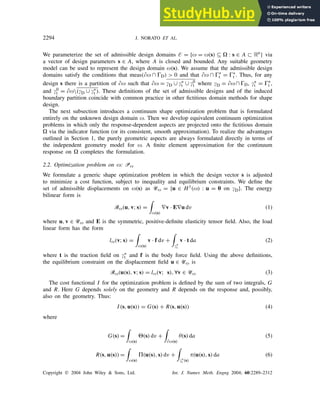
Figure 1. Physical problem domain embedded in the fictitious domain .
analysis methods, such as the material distribution methods commonly used in topology op-
timization. Geometric properties are readily and unambiguously available, and as is typical
with direct geometry models, a relatively small number of design parameters can represent the
design domain. At the same time, the response analysis can exploit all of the well-known ad-
vantages of fictitious domain methods, including simplified mesh generation, no mesh tangling
or element distortion due to design changes, and the option to use efficient solvers that are
designed for structured meshes.
Fictitious domain methods simplify response analysis problems by embedding a complicated
problem domain in a larger, but simpler, ‘fictitious’ domain (see Figure 1). A proxy
analysis problem is then formulated and solved on , such that the restriction of the proxy
solution to is equivalent to the solution of the original problem. Meshless methods sometimes
use a similar approach (cf. Reference [1]).
In functional analytical fictitious domain methods, the proxy problem on includes con-
straints that enforce the boundary conditions of the original problem on *. The proxy prob-
lem is typically formulated as a constrained minimization problem; techniques for solving this
problem include the distributed optimal controls method [2], the boundary Lagrange multiplier
method [3], and the distributed Lagrange multiplier method [4]. In numerical implementations
of the Lagrange multiplier methods, the discrete response models for the fictitious domain
and for * must be carefully chosen to satisfy the Ladyshenskaja–Babushka–Brezzi (LBB)
condition [5].
Material projection versions of the fictitious domain method introduce a material measure
that reflects the distribution of solid and void subregions within .‡ Sometimes the material
measure also models homogeneous Dirichlet boundary conditions [6–8]. The material measure
‡These methods typically circumvent the aforementioned LBB condition.
Copyright 䉷 2004 John Wiley Sons, Ltd. Int. J. Numer. Meth. Engng 2004; 60:2289–2312

GEOMETRY PROJECTION METHOD FOR SHAPE OPTIMIZATION 2291
can be defined simply as the characteristic function associated with , or it can take the form
of a continuous mapping that assigns intermediate values to material points near the boundary
of .
Some researchers have applied functional-analytical fictitious domain methods in the context
of the boundary-variation approach to shape optimization [5, 9–11]. A lack of differentiability of
the response with respect to the control has been reported in some numerical implementations.
Also, the difficulty of satisfying the LBB condition is exacerbated as the domain varies
during the optimization process.
Material distribution methods [12, 13] are closely related to material projection fictitious
domain methods and are the cornerstone of successful numerical techniques for topology op-
timization. In these methods, the material distribution (measure) is the control; it is defined
directly as in a grey-scale raster image, rather than as a projection of a classical geome-
try model. The geometry must be inferred from the material distribution, as in certain
image processing problems. Response solutions are typically computed by the finite element
method,§ with at least one material parameter assigned to each element. Although this approach
generates a large number of design parameters, it does allow for the evolution of both topology
and shape (within the framework of the raster representation). However, a well-defined inverse
material projection that maps a material distribution into a classical geometry representation
is lacking in these methods. This makes it difficult to evaluate geometric properties, such
as perimeter and curvature, and to enforce various mechanical conditions that depend on the
precise properties of the boundaries of the varying domain .
Recently, level set methods have been applied to shape design and especially to topology
optimization. Sethian and Wiegmann [15] combine the level set geometry model with an ad
hoc optimality criterion based on the Von Mises equivalent stress for the transport of the level
set function. Allaire et al. [16] and Wang et al. [17] work with well-defined objective functions
and follow approaches that are similar to the one proposed here in that they employ a geometry
projection based on the level set model. However, their formulations and solution procedures
are specific to the level set methodology, whereas the one proposed here can be combined with
any suitable geometry model and with any optimization algorithm. The latter level set methods
are able to change topology by merging holes. However, as indicated in Reference [16], they
are so far unable to introduce new holes. Level set methods involve implicit geometry models;
Belytschko et al. [18] also use an implicit geometry model to describe designs with varying
connectivity. They modify the material model in a finite band surrounding the design boundary
to obtain a more robust method that is better able to introduce holes as well as to remove them.
The modified material model imposes an implicit penalty on intermediate values of the level-
set function, and is similar to the material models used in so-called SIMP methods (see, for
example, Reference [12]). A discussion of implicit penalties in the context of variable-topology
shape optimization can be found in Reference [19].
The method advanced in this paper combines a classical geometry model for the physical
domain with a filtering technique that projects onto a convenient fictitious domain . The
natural parameterization of the geometry model’s design space is the control in the optimization
problem; the projection onto the fictitious domain is only used for the purposes of response
analysis and response sensitivity analysis. All geometric quantities, such as volume, perimeter,
§Wavelet methods have also been used for this purpose [14].

Figure 2. (a) Classical geometric design model; and (b) raster analysis model.
surface normal, boundary curvature and the corresponding sensitivities are computed directly
from the geometry model; there is never a need to infer geometry from the projected model.
We can use any suitable mathematical programming method to solve the optimization problem.
To facilitate the optimization process, we favor geometry models and filter definitions such
that the relevant geometric properties, the geometry projection and the system response are
all differentiable with respect to the control. To this end, we use a smooth filtering of the
indicator function for to define the geometry projection. The filter is based on a bounded
sample window whose diameter is proportional to the local grid spacing in the numerical mesh
used for response analysis. Thus, the errors associated with both the geometry projection and
the response discretization vanish in the limit of numerical mesh refinement. Accordingly, the
numerical response solution converges to the continuum solution of the underlying boundary
value problem.
To exemplify the method, we consider a linearly elastic square plate with an elliptical hole
that is subjected to in-plane traction loads (see Figure 2(a)). The control parameters are the
ellipse radii (a, b). We seek a design that minimizes the compliance, subject to a constraint
on the volume and box constraints on the radii. The sensitivities of the volume with respect
to the control parameters are computed analytically. We use the geometry projection and a
regular finite element grid that covers to evaluate the compliance and its sensitivity (see
Figure 2(b)).
In the following section, we present a continuum shape optimization problem on for lin-
early elastic structures. We develop an equivalent fictitious domain formulation for the response
analysis that uses the indicator function for to define a geometry projection onto . Then we
introduce two approximations that facilitate the numerical solution of the system response and
the optimization problem. First, we filter the indicator function to define a modified projection
that guarantees the differentiability of the system response with respect to the original shape
parameters for . The modified projection agrees with the indicator function, in the limit, as the
diameter of the filter sample window goes to zero. Second, we introduce a finite element ap-
proximation for the response solution on and make the diameter of the filter sample window
proportional to the local element diameter. This ensures that both the finite element response
approximation and the numerical solution to the overall optimization problem converge to their
continuum counterparts in the limit of grid refinement. We emphasize that only the response
solution need be approximated in this development; the original design parameters that describe
still control the shape optimization problem, and we use the analytical geometry model as
the basis for the evaluation of all geometric quantities.

Section 3 presents numerical examples that demonstrate the performance and convergence
properties of our method for the elliptical-hole design problem described above. We consider
two shape optimization problems: one for minimum compliance subject to a volume constraint
and one for minimum volume subject to a constraint on the maximum von Mises effective
stress. Section 4 presents a shape optimization example for a bridge structure to demonstrate
the design capabilities of our method. In contrast to the explicit model used in Section 3, we
use an implicit geometry model based on radial basis functions to meet the more demanding
requirements of the bridge design problem.
2. PROBLEM FORMULATION
2.1. Domain definitions
We restrict our attention to linearly elastic structural shape optimization problems with design-
independent surface loads¶ and homogeneous Dirichlet boundary conditions (cf. Figure 3),
where (a) the boundary region with applied non-homogeneous tractions is fixed and finite,
and (b) the Dirichlet boundary region is variable, but restricted to a specified portion of *.
The restrictions to linearly elastic material response and to homogeneous Dirichlet boundary
conditions are adopted to simplify the presentation and are not intrinsic limitations of the
method.
Let ⊂ En
be the fictitious domain, and let = *. We partition into two complementary
regions, D and t, on which the Dirichlet and the traction boundary conditions are applied. The
traction boundary is further subdivided into the complementary regions 0
t and ∗
t , on which
the homogeneous and non-homogeneous tractions are prescribed (for simplicity, we assume that
the non-homogeneous tractions act on ; however, they could also be prescribed on a specified
part of *).
Our purpose here is to formulate shape optimization problems in which the fictitious domain
is the admissible design region. That is, any admissible design must satisfy ⊆ .
Figure 3. Identification of the physical domain , the fictitious domain and the prescribed-traction
and prescribed-displacement portions of their boundaries.
¶We intend to extend the method to address design-dependent surface tractions in our continuing research.

We parameterize the set of admissible design domains O = { = (s) ⊆ : s ∈ A ⊂ Rn
} via
a vector of design parameters s ∈ A, where A is closed and bounded. Any suitable geometry
model can be used to represent the design domain (s). We assume that the admissible design
domains satisfy the conditions that meas(* ∩ D) 0 and that * ∩ ∗
t = ∗
t . Thus, for any
design s there is a partition of * such that * = D ∪ ∗
t ∪ 0
t where D = * ∩ D, ∗
t = ∗
t ,
and 0
t = *(D ∪ ∗
t ). These definitions of the set of admissible designs and of the induced
boundary partition coincide with common practice in other fictitious domain methods for shape
design.
The next subsection introduces a continuum shape optimization problem that is formulated
entirely on the unknown design domain . Then we develop equivalent continuum optimization
problems in which only the response-dependent aspects are projected onto the fictitious domain
via the indicator function (or its consistent, smooth approximation). To realize the advantages
outlined in Section 1, the purely geometric aspects are always formulated directly in terms of
the independent geometry model for . A finite element approximation for the continuum
response on completes the formulation.
2.2. Optimization problem on : P
We formulate a generic shape optimization problem in which the design vector s is adjusted
to minimize a cost function, subject to inequality and equilibrium constraints. We define the
set of admissible displacements on (s) as U = {u ∈ H1() : u = 0 on D}. The energy
bilinear form is
B(u, v; s) =

(s)
∇v · E∇u dv (1)
where u, v ∈ U and E is the symmetric, positive-definite elasticity tensor field. Also, the load
linear form has the form
l(v; s) =

(s)
v · f dv +

∗
t
v · t da (2)
where t is the traction field on ∗
t and f is the body force field. Using the above definitions,
the equilibrium constraint on the displacement field u ∈ U is
B(u(s), v; s) = l(v; s), ∀v ∈ U (3)
The cost functional I for the optimization problem is defined by the sum of two integrals, G
and R. Here G depends solely on the geometry and R depends on the response and, possibly,
also on the geometry. Thus:
I(s, u(s)) = G(s) + R(s, u(s)) (4)
where
G(s) =

(s)
(s) dv +

*(s)
(s) da (5)
R(s, u(s)) =

(s)
(u(s), s) dv +

∗
t (s)
(u(s), s) da (6)

in which it is understood that , , , and are fields that depend explicitly on position x,
and that *∗
t is also a function of the design vector s.
The optimization problem involves m constraint functionals gi, i = 1 . . . m that are given
as
gi(s, u(s)) = Gi(s) + Ri(s, u(s)) (7)
where Gi and Ri are defined analogously to G and R. Note that the integrands in G and Gi
are explicit functions of the design geometry, while the integrands in R and Ri are implicit
functions of the geometry via the response u. These formats for the objective function and for
the constraints support descriptions of common geometric measures, such as volume ( = 1)
and perimeter ( = 1).
The optimization problem on is then stated as
P















min
s∈A
I(s, u(s))
s.t. u(s) ∈ U
B(u(s), v; s) = l(v; s) ∀v ∈ U
gi(s, u(s)) 0, i = 1, 2, . . . , m
(8)
We emphasize that the integrals in I, gi, B and l are defined on and that the vector s is
the control in this problem. We retain s as the control throughout the subsequent development.
The geometry model is assumed to have sufficient compactness and smoothness properties
to assure that the continuous problem P has a solution along the lines described in Haslinger
and Neittaanmäki [5]. A typical CAD geometry model that is based on a closed and bounded
design set A in Rn
satisfies this assumption.
2.3. Optimization problem on : P
We next formulate a shape optimization problem that is equivalent to P, where the response
is obtained via a geometry projection onto the fictitious domain . Letting U = {u ∈ H1() :
u = 0 on D} be the set of admissible displacements on , we replace the energy bilinear
form and the load linear form in Equations (1) and (2) with
B(u, v; s) =

∇v · E∇u dv (9)
l(v; s) =

v · f dv +

*∗
t
v · t da (10)
Point-wise constraints can be defined using the Dirac delta function. Also, we intend that and i might
depend on ∇u.

where u, v ∈ U. Also, is the indicator function for (s); that is,
(x; s) =

1 if x ∈ (s)
0 if x ∈ (s)
(11)
We replace the equilibrium constraint (3) with an equivalent constraint on û, the extension
of the displacement solution to . That is, for û ∈ U we require
B(û(s), v; s) = l(v; s) ∀v ∈ U (12)
The inclusion of in the bilinear form B and the conditions imposed on the boundaries
ensure that the restriction of û to equals the desired solution, i.e. û| = u.
In light of the above, the cost and constraint functions of Equations (4) and (7) are replaced,
respectively, by the equivalent functions
ˆ
I(s, û(s)) = G(s) + R̂(s, û(s)) (13)
and
ĝi(s, û(s)) = Gi(s) + R̂i(s, û(s)) (14)
where
R̂(s, û(s)) =

(s)(û(s), s) dv +

∗
t
(û(s), s) da (15)
A similar expression defines R̂i. It is clear from Equation (11) that Equations (13) and (14)
are equivalent to Equations (4) and (7), respectively.
The equivalent optimization problem on the fictitious domain is
P















min
s∈A
ˆ
I(s, û(s))
s.t. û(s) ∈ U
B(û(s), v; s) = l(v; s) ∀v ∈ U
ĝi(s, û(s)) 0, i = 1, 2, . . . , m
(16)
The equilibrium problem for û is not well-posed because the displacement solution in the
complement of is not unique. Nonetheless, the optimization problem makes sense because
û| is unique.
We emphasize that the control in P is the design vector s, and not the indicator function
. That is, we use an independent geometry model to describe (s) and obtain from ,
as opposed to inferring from . In numerical implementations, this facilitates the evaluation
of geometric properties, such as the volume and perimeter of . In addition, fewer design
variables are generally required to parameterize than .
2.4. Smooth approximations of
We approximate the indicator function with a smooth, positive function that depends
smoothly on the design vector s to simplify the implementation. This approximation is computed

Figure 4. Unfiltered volume fraction
and its derivative ′
for a square sample window centred at
x and aligned with *. The parameter s denotes the distance between x and *.
by first filtering , using a suitably smooth filter with compact support, to obtain a volume
fraction distribution
.∗∗ Then we use
to construct a geometry measure, ,
: → [ , 1],
in which 0 and 0 1. We require that ,
is smooth in s and continuous in and
, such that lim, →0+ ,
= . The lower bound on the range of ,
guarantees that the
energy bilinear form in (12) is positive definite, which ensures that the corresponding analysis
problem on is well posed.
The simplest filter is the volume fraction,

(x; s) =
meas(R
x ∩ )
meas(R
x ∩ )
(17)
in which R
x is an open sample window of diameter 2 that is centred at x. Note that
lim→0+
= (in L2()). To obtain ,
, we write
,
(x; s) = + (1 − )
(x; s) (18)
The definition of
in (17) is differentiable with respect to the design in most situations.
But if, for example, a part of * contains a straight edge and the sample window is a square
with one side parallel to that edge, then the design derivative of
is discontinuous with
respect to normal motions of *, as illustrated in Figure 4. The use of a filter with better
smoothness properties can circumvent this problem. For example, the simple volume fraction

in (17) can be replaced by

(x; s) =

(y; s)K(x − y) dy (19)
∗∗A similar idea is suggested in Reference [20], but has not, to our knowledge, been pursued further.

Figure 5. Filtered volume fraction
and its derivative ′
for a square sample window centred at x
and aligned with *. The parameter s denotes the distance between x and *.
where K is a continuous, non-negative convolution kernel such that the support of K is R
0
and K|R
0
is smooth.†† In particular, the ‘bubble’ kernel function,
K(x) =





9
166
(x2
1 − 2
)(x2
2 − 2
) if x ∈ R
0
0 otherwise
(20)
defined on an open square filter window of size 2 yields the filtered volume fraction depicted
in Figure 5.
We use the filtered geometry measure ,
to define a proxy optimization problem for P:
P ,
















min
s∈A
˜
I(s, û(s))
s.t. û(s) ∈ U
B ,
(û(s), v; s) = l ,
(v; s) ∀v ∈ U
g̃i(s, û(s)) 0, i = 1, 2, . . . , m
(21)
where
˜
I(s, û(s)) = G(s) + R̃(s, û(s)) (22)
g̃i(s, û(s)) = Gi(s) + R̃i(s, û(s)) (23)
††K is similar to a mollifier (see, for example, Reference [21]), except we do not require its derivative to
vanish on *R
0.

R̃(s, û(s)) =

,
(s) (û(s)) dv +

∗
t
(û(s)) da (24)
B ,
(u, v; s) =

,
(s)∇v · E∇u dv (25)
l ,
(v; s) =

,
(s)v · f dv +

*∗
t
v · t da (26)
in which u, v ∈ U, and R̃i is defined similarly to R̃. In contrast to many other fictitious
domain methods, there is no penalization (implicit or explicit) of the intermediate densities.
Instead, the parameter directly controls the extent of regions with intermediate density. Indeed,
as , → 0+, ,
approaches , and û| approaches u. Therefore, we expect the solution of
P ,
to approach the solution of P as , → 0+ when the existence of a solution is assured
for both problems.
The modified problem P ,
facilitates implementations of shape optimization algorithms
relative to problems P and P. In the classical techniques of shape sensitivity analysis (see,
e.g., References [22, 23]) one works directly with the problem P to compute the derivatives
of the objective and constraint functions with respect to the control s. This requires careful and
repeated remeshing of the design domain (s) within an iterative optimization procedure. For
the fictitious domain formulations, P and P ,
, we base our analysis on a fixed mesh on that
does not depend on s. This simplifies the sensitivity analysis, as explained below. However, the
objective and constraint functions in P can be non-smooth (or even discontinuous, depending
on the implementation) with respect to the design vector s, an undesirable property that calls for
a more sophisticated and more expensive optimization algorithm. The smooth filter introduced
in P ,
circumvents this problem, thereby supporting the use of simpler and more efficient
optimization routines.
2.5. Sensitivity analysis
The derivatives of the cost function with respect to s follow from Equation (22):
D ˜
I
Ds
=
DG(s)
Ds
+
DR̃(s, û(s))
Ds
(27)
where
DR̃(s, û(s))
Ds
=

,

*
*û
Dû
Ds
+
*
*s
+ ,′

D

Ds
dv+

∗
t

*
*û
Dû
Ds
+
*
*s
da (28)
We use the underlying analytical geometry model to compute the derivatives DG/Ds, */*s,
*/*s and D
/Ds directly. This circumvents problems associated with inferring the fine
details of the geometry, such as the precise location and orientation of *, from a rasterized
representation of the geometry measure ,
. The equilibrium constraint in Equation (21) is
eliminated by performing a design sensitivity analysis. The implicit response derivative Dû/Ds
in Equation (28) is subsequently annihilated or evaluated by using either the adjoint or the
direct method [24]. We compute the derivatives of the constraint functions in a similar manner.

2.6. Finite element approximation
We use a standard Galerkin finite element approximation to evaluate the displacement field on
for a given design , as specified by the control vector s. In our current implementation,
we use a uniform mesh of square bilinear elements with edge-length h. A key requirement
is that the solution to the discrete optimization problem must converge to the solution of the
original optimization problem P in the limit of mesh refinement. To this end, we specify
the diameter of the filter sample window as a function of the element size, = ˆ
(h), such
that → 0+ monotonically as h → 0+. Thus, the geometry measure ,
converges to in
L2(), in the limit, as h, → 0+. As with other fictitious domain methods, a suitable lower
bound for must be imposed (with due consideration of machine precision) to avoid numerical
ill-conditioning.
We define the discrete optimization problem P ,h
by restricting the discrete displacement
solution uh to a finite-dimensional subspace of U, and by replacing ,
in P ,
with
,ˆ
(h)
.
It can be proved by standard arguments that, for a fixed design, the finite element displacement
solution converges to the continuum solution in the limit of mesh refinement. Further, the
techniques advanced by Haslinger and Neittaanmäki [5] prove that, for a standard setting of
the shape design problem, the solution to the discrete optimization problem P ,h
converges
(i.e., there exists a subsequence that converges) to the solution of the continuum problem P
in the limit.‡‡ We verify this result via numerical experiments in the following section.
3. NUMERICAL CONVERGENCE STUDIES
3.1. Design of a plate with an elliptical hole
This section presents a numerical study of the convergence properties of the proposed shape
optimization method. To this end, we select a simple optimization problem for which analytical
solutions for the optimal designs are available. Specifically, we consider the problem of op-
timizing the radii of an elliptical hole at the centre of a square plate of unit thickness that
is comprised of a homogeneous, isotropic and linearly elastic material. The plate is subjected
to plane-stress, bi-axial loading, as shown in Figure 6, and we enforce symmetry conditions
to restrict the model to one quarter of the plate. The plate’s dimensions, material properties
and certain convergence tolerances are shown in Table I. §§ We investigate two optimization
problems: (a) minimize the compliance subject to a constraint on the volume, and (b) minimize
the volume subject to a constraint on the maximum von Mises stress. We invoke a conjugate
gradient algorithm with element-by-element Gauss–Seidel preconditioning to solve the equilib-
rium problem, and use the method of moving asymptotes (MMA) [25] to solve the optimization
problems.
‡‡This convergence property holds for the true minima of the design problems. However, as with any continuum
design problem, computational optimization methods typically are only guaranteed to generate local minima.
§§The convergence tolerance for the objective function applies to the absolute value of the change due to
the most recent design update, normalized by the current value. The convergence tolerance for the equilibrium
residual applies to the ratio of the norms of the residual nodal force vector and the applied nodal-force
vector.

Figure 6. Square plate with an elliptical hole subjected to uniform normal tractions.
Table I. Material properties, dimensions, and convergence criteria.
Young’s modulus, E 10 N/mm2
Poisson ratio, 0.3
l 10 mm
Plate thickness 1 mm
1E-8
Convergence tolerance for objective function 1E-8
Convergence tolerance for equilibrium residual 1E-6
An explicit representation of the boundary of the elliptical hole provides a convenient, two-
parameter representation of the design space.¶¶ Any point ys on the ellipse is described by
ys() =

a cos ()
b sin ()
in which the principle radii of the ellipse comprise the control vector s = (a, b) ∈ A =
[0, l] × [0, l].
We introduce two simplifications in this example to facilitate our numerical implementation.
First, the geometry measure
,ˆ
(h)
is taken to be uniform over each element, based on the value
at the element centroid. Thus, for each element, the filter sample window is the ball with
radius = (
√
2/2)h that circumscribes the element.∗∗∗ Second, we use a local approximation
¶¶The proposed method does not require an explicit geometry model; the next section presents an example
based on an implicit geometry model.
Henceforth, we omit the subscript and the superscripts on for simplicity.
∗∗∗The union of the sample windows must be a covering of to avoid situations in which the geometry
measure is artificially insensitive to certain design changes.

Table II. Optimal designs for symmetric load.
Mesh a(mm) |a − R|/R b(mm) |b − R|/R ˜
Ih(N mm)
16 × 16 6.19537 0.00242502 6.16544 0.00241916 32.3305
32 × 32 6.18037 2.39841E-06 6.18040 2.39841E-06 32.3855
64 × 64 6.18041 2.92869E-06 6.18037 2.92865E-06 32.3904
of * to compute the volume fraction
. Specifically, we replace the exact local geometry
of * with its tangent plane at the location determined by the nearest-point projection of the
centre of each sample window to *.
3.2. The compliance problem
The goal in this problem is to find the ellipse that minimizes the compliance subject to a
maximum volume constraint (specified as an allowable percentage p of the volume of the plate
with no hole). The optimization problem P is stated as
min
s∈A
ˆ
I(s) =

∗
t
û(s) · t da
s.t. û(s) ∈ U
ĝ1(s) = (1 − p)l2
−
ab
4
0
B ,
(û(s), v; s) = l ,
(v; s) ∀v ∈ U
(29)
Since this problem involves only the objective and one constraint function, we use the adjoint
method of sensitivity analysis in our computations.
3.2.1. Symmetric load. We first consider the case of an isotropic load with p = 70%. The
optimal design is symmetrical, a = b = R, in which the volume constraint requires that
R = l[(4/)(1 − p)]1/2. For the given values of l and p, we find that R = 6.180387 mm. We
used Fx = Fy = −1 N/mm in our computations (see Figure 6) and specified an asymmetric
and feasible initial design, a = 9 mm, b = 4.5 mm. The optimization results appear in Table II
for 16×16, 32×32 and 64×64 meshes; plots of the corresponding optimal geometry measures
are shown in Figure 7.
3.2.2. Convergence study. We performed convergence studies for the geometry measure and
the compliance to determine the accuracy of our numerical method. Since we are ultimately
interested in obtaining a black and white design with sharp boundaries, we define a geometric
sharpness error to quantify the amount of grey volume in the filtered model:
eg =
4
v

(1 − ) dv (30)
where v is the volume of . The sharpness error will be unity if = 0.5 almost everywhere
on , and it will vanish if is either zero or unity almost everywhere on . The geometric

Figure 7. Geometry measure distributions at the optimal design, symmetric load case:
(a) 16 × 16 mesh; (b) 32 × 32 mesh; and (c) 64 × 64 mesh.
Table III. Convergence study for symmetric loading.
h (mm) Ch (N mm) eg (%) eC (%) ev (%) Nodes Elements
2 31.3961 14.5354 −3.0312 −0.351427 36 25
1 32.2919 7.6067 −0.2645 −0.241073 121 100
0.5 32.3681 4.0195 −0.0289 −0.055863 441 400
0.25 32.3903 2.0032 0.0395 −0.009005 1681 1600
0.125 32.3899 0.9993 0.0382 −0.007768 6561 6400
0.0625 32.3824 0.4936 0.0151 0.000945 25 921 25 600
0.03125 32.3800 0.2499 0.0076 0.000427 10 3041 10 2400
−1 −0.5 0 0.5 1 1.5 2 2.5 3 3.5
−5.5
−5
−4.5
−4
−3.5
−3
−2.5
−2
log(1/h)
log
|e
g
|
49
50
Figure 8. Convergence of the geometric sharpness error with respect to mesh refinement.
sharpness errors for different meshes at the optimal design (i.e., a circular hole of radius
R = 6.180387 mm) appear in Table III and are plotted in Figure 8. Figure 9 shows the
distributions at the optimal design on the 64 × 64 mesh of the geometry measure and the
geometric sharpness error density (4(1 − )).

Figure 9. Optimized design for a 64 × 64 mesh: (a) geometry measure ;
and (b) geometric sharpness error density.
−2 −1 0 1 2 3 4 5
−9
−8
−7
−6
−5
−4
log(1/h)
log
|e
C
|
99
100
337
100
Figure 10. Convergence of the compliance error with respect to mesh refinement.
We define the normalized compliance error as
eC =
Ch − Cref
Cref
(31)
where Ch denotes the compliance of the finite element solution on the fictitious domain , and
Cref is a reference value that closely approximates the compliance of the exact optimal solution.
Since there is no analytical solution available for the compliance, we use a highly refined finite
element mesh that is fitted to the exact optimal geometry to compute Cref. Using ABAQUS䉸
and a mesh with 10240 8-node bi-quadratic finite elements, we obtain Cref = 32.3775 N mm.
Table III and Figure 10 show the convergence results for the compliance error.

−2 −1 0 1 2 3 4 5
−12
−11
−10
−9
−8
−7
−6
log(1/h)
log
|e
v
|
23
20
211
100
Figure 11. Convergence of the normalized volume error with respect to mesh refinement.
As a further check of the accuracy of the geometry projection, we introduce a measure
of the difference between the integral of the geometry measure at the optimal design and
the maximum allowable volume specified in the optimization problem. Thus, we define the
normalized volume error as
ev =
1
pv

dv − 1 (32)
Convergence results for the volume error also appear in Table III, and are plotted in Figure 11.
As seen in Figure 8, the geometric sharpness error is proportional to the element size h, and
this fact limits the asymptotic convergence rate of the compliance, as seen in Figure 10. The
non-smooth feature in Figure 10 is attributed to a change in sign of the compliance error and a
transition from a regime in which the response discretization error dominates to an asymptotic
regime in which the geometry error dominates.
3.2.3. Asymmetric load. Here we consider an asymmetric load given by Fy = 2Fx = −2
N/mm. We compare our computational results for the finite plate with the analytical solution
for the optimal design of an infinite plate with an elliptical hole subject to the same biaxial
stress state as a far-field loading (see for example Reference [26]). The optimal design for the
infinite plate is
b
a
=
Fy
Fx
= 2 (33)
We choose a relatively large allowable volume, p = 95%, to obtain a better approximation of
the infinite plate solution. Table IV shows results obtained with 16 × 16, 32 × 32 and 64 × 64
meshes; Figure 12 shows the optimal distribution of the geometry measure for the 64 × 64
mesh. Our numerical results differ from the reference infinite-plate design by at most 6%. We
do not expect precise agreement, because the optimal designs for the finite and infinite plates
are distinct [26].

Table IV. Optimal designs for asymmetric loading; q = (b/a)ref = 2.
Mesh a (mm) b (mm) b/a (q − b/a)/q ˜
Ih (N mm)
16 × 16 1.79143 3.55369 1.98372 0.8142% 42.6738
32 × 32 1.84054 3.45888 1.87927 6.0363% 42.7542
64 × 64 1.81278 3.51184 1.93727 3.1366% 42.7770
Figure 12. Optimal geometry measure distribution for the asymmetric load case on the 64 × 64 mesh.
3.3. Stress concentration problem
In this example, we seek the ellipse that minimizes the plate volume subject to a system
of point-wise constraints that approximates an L∞ constraint on the von Mises stress. The
optimization problem P is stated as
min
s∈A
ˆ
I(s) = l2
−
ab
4
s.t. û(s) ∈ U
ĝi(s) =

(x; s) (x − xi) (x; s) dv − max 0, i = 1, . . . , n
B ,
(û(s), v; s) = l ,
(v; s) ∀v ∈ U
(34)
where is the equivalent von Mises stress field, max is the allowable von Mises stress and
n is the number of point-wise stress constraints. In the discrete finite element version, we set
n equal to the number of elements and identify xi with the centroid of element i. Given the
large number of constraint functions in this problem, we use the direct method of sensitivity
analysis in our computations.

Table V. Optimal designs for stress constraint with symmetric loading.
Mesh a (mm) b (mm) volume (mm3)
16 × 16 6.0268 6.0498 71.364
32 × 32 5.5003 5.5003 76.239
64 × 64 5.2950 5.2546 78.148
128 × 128 5.1266 5.1266 79.357
Table VI. Optimal designs for stress constraint with asymmetric loading; q = (b/a)ref = 2.
Mesh a (mm) b (mm) b/a (q − b/a)/q (%) volume (mm3)
16 × 16 2.6480 5.6656 2.1396 −6.9792 88.217
32 × 32 2.1458 4.5837 2.1361 −6.8044 92.275
64 × 64 1.7387 3.6994 2.1276 −6.3815 94.948
3.3.1. Symmetric load. We consider a uniform isotropic load, Fx = Fy = −1N/mm, and, again,
we expect to generate a symmetric optimal design, a = b = R∗. However, in contrast to the
compliance minimization problem, there is no analytical result available for the optimal radius
R∗ in this case. Instead, we use ABAQUS䉸 to analyze a plate with a circular hole of radius
R = 5 mm; using a mesh consisting of 11680 8-node elements, we obtain a maximum von
Mises stress of 2.732051N/mm2. We assign this value to max in (34), and expect the resulting
optimization problem to yield an optimal hole radius of roughly R∗ = 5 mm. This is equivalent
to an optimal volume (for the quarter plate) of 80.365 mm3. We begin our computations with
an asymmetric initial design: a = 0.1 mm, b = 1.0 mm. Table V displays the optimization
results for 16 × 16, 32 × 32, 64 × 64, and 128 × 128 meshes.
3.3.2. Asymmetric load. For an asymmetric load, Fy = 2Fx = −2 N/mm, we expect our com-
putational results to nearly agree with the optimal design for an infinite plate (cf. Equation (33)).
To better approximate the infinite-plate result, we assign max = 3N/mm2 to cause the optimal
volume to be a relatively high percentage of the plate volume. The results for the 16 × 16,
32 × 32 and 64 × 64 meshes are presented in Table VI.
4. OPTIMIZATION EXAMPLE
We next present numerical results that demonstrate the design capabilities of the proposed
method. We consider a shape optimization problem that emulates the elegant three-hinge-arch
bridge designs of the Swiss engineer, Robert Maillart. In contrast to the explicit boundary
representation used in the previous section, here we use an implicit geometry model to ac-
commodate a wider variety of shapes. Specifically, * is identified with the zero-level set
of a scalar function f , such that = {x ∈ : f (x) 0} [27]. We use thin-plate radial
basis functions centred on a prescribed set of constraint-point locations {ci} to model f . This
representation guarantees desirable smoothness properties for *. We identify the values of f
at the constraint-point locations with the elements of the design vector s: si = f (ci). Since

Figure 13. The bridge-design problem: geometry, support conditions, loads and constraint-point
locations (◦) for the radial basis functions.
the implicit model offers no natural parameterization of the boundary, we use a polygonization
technique [28] to construct a piecewise-linear approximation of *.
The volume fraction computations in this example are based on square sample windows that
coincide with individual finite elements, and the volume fraction is approximated as uniform
over each element. The bubble function of Equation (20) defines the kernel of the integral in
(19). We use the polygonal approximation of * and Gauss’ theorem to evaluate the integral,
as described in Reference [29]. All other geometric properties are computed directly from the
polygonal approximation of * (using Gauss’ theorem where appropriate).
The bridge-design problem is diagrammed in Figure 13. Fixed support conditions are available
at the left-edge top and bottom corners, and symmetry conditions are prescribed along the right
edge of the fictitious domain (which models only the left half of the structure). The top edge
carries a uniform, distributed vertical load, while the bottom edge is unloaded and unsupported.
The homogeneous elastic material properties are the same as those listed in Table I, and a 72×36
grid of square finite elements with bilinear basis functions discretizes the fictitious domain for
the response analysis. We seek a shape design that minimizes the compliance subject to a
resource constraint that limits the design to 30% of the fictitious domain area. Figure 13 also
shows the grid of 315 constraint-point locations; the values of f at these locations comprise
the elements of the design vector s. The constraint-point grid extends beyond the fictitious
domain to avoid inadvertent constraints on the shape of near the boundary of .
We use the MMA algorithm to carry out the shape optimization, and we terminate the design
iterations when the relative change in compliance is less than 1 × 10−6 for two consecutive
iterations. Figure 14 shows a sequence of designs generated during the optimization. The final

Figure 14. Initial, intermediate, and final designs for the bridge-design problem: (a) initial design; (b)
iteration 10; (c) iteration 20; (d) iteration 40; (e) iteration 60; and (f) iteration 117 (final design).
Figure 15. Scalar function f and physical domain in the implicit geometry model; initial design.

Figure 16. Scalar function f and physical domain in the implicit geometry model; final design.
design is attained in 117 iterations, and it is similar to some of Maillart’s bridge designs.
Figures 15 and 16 present plots of the function f over the fictitious domain for the initial
and final designs; the corresponding physical domains are also shown.
5. CONCLUSIONS
The numerical results confirm that solutions obtained with the new method converge to solutions
of the underlying continuum optimization problem in the limit of mesh refinement. However,
the geometry projection, which must ultimately resolve the discontinuous indicator function,
limits the asymptotic convergence rate to O(h). This suggests that adaptive analysis techniques
could improve the efficiency of the method. In particular, the independence of the geometry
and response models admits the possibility of independent adaptive refinement of the finite
element mesh and the grid of control points in the geometry model. Our method is robust in
the sense that it is compatible with any analytical geometry model (both implicit and explicit
geometry models are supported), with any response analysis method (not necessarily a finite
element method) and with any optimization algorithm.
Since the degree of mesh refinement controls the resolution of the geometry projection on the
fictitious domain, there is no need to introduce a penalty on intermediate values of the geometry
measure to achieve a black and white design. In particular, our method does not artificially
modify the material properties to achieve an implicit penalty against intermediate values of the
geometry measure (as in, for example, the SIMP method for variable-topology design). This

could be an advantage in optimization problems that involve dynamics or vibrations, where
non-physical interpolations of the material density and the material stiffness properties might
alter the wave speeds and the vibration modes.
Applications of the new method to variable-topology shape optimization are a natural ex-
tension of the work reported here. Implicit geometry models, such as the one used in the
bridge-design example, easily accommodate changes in connectivity. The critical new capabil-
ity required for a robust topology algorithm is a strategy for adding and deleting holes at
appropriate stages of the optimization process.
ACKNOWLEDGEMENTS
Support from the University of Illinois Center for Process Simulation and Design (CPSD) is gratefully
acknowledged. The U.S. National Science Foundation supports research in CPSD via Grant NSF
DMR 01-21695. The first author thanks the Fundación para el Futuro de Colombia, COLFUTURO,
for partial support of his graduate studies. The support of the second author by the Technical University
of Denmark and the Otto MZnsted Foundation is also gratefully acknowledged. We thank Prof. Krister
Svanberg of the Department of Mathematics, KTH Stockholm for allowing us to use his implementation
of the method of moving asymptotes for the optimization examples in this work. We also thank Prof.
John C. Hart, Department of Computer Science, University of Illinois at Urbana-Champaign for his
advice on implementation of the implicit geometry model with radial basis functions.
REFERENCES
1. Liu WK, Jun S, Zhang YF. Reproducing kernel particle methods. International Journal of Numerical Methods
in Fluids 1995; 20:1081–1106.
2. Atamian C, Dinh GV, Glowinski R, He J, Periaux J. On some imbedding methods applied to fluid dynamics
and electro-magnetics. Computer Methods in Applied Mechanics and Engineering 1991; 91:1271–1299.
3. Glowinski R, Pan TW, Periaux J, A fictitious domain method for Dirichlet problems and applications.
Computer Methods in Applied Mechanics and Engineering 1994; 111:283–303.
4. Glowinski R, Pan TW, Periaux J, A fictitious domain method for external incompressible viscous flow
modeled by Navier–Stokes equations. Computer Methods in Applied Mechanics and Engineering 1994;
112:133–148.
5. Haslinger J, Neittaanmäki P. Finite Element Approximation for Optimal Shape, Material and Topology Design
(2nd edn). Wiley: Chichester, 1996.
6. Bakhvalov NS, Knyazev AV. Fictitious domain methods and computations of homogenized properties
of composites with a periodic structure of essentially different components. In Numerical Methods and
Applications, Marchuk GI (ed.). CRC Press: Boca Raton, FL, 1994; 221–226.
7. García-Ruíz MJ, Steven GP. Fixed grid finite elements in elasticity problems. Engineering Computations
1999; 16(2):145–164.
8. Belytschko T, Möes N, Usui S, Parimi C. Arbitrary discontinuities in finite elements. International Journal
for Numerical Methods in Engineering 2000; 50:993–1013.
9. Haslinger J. Comparison of different fictitious domain approaches used in shape optimization. Technical
Report 15, Laboratory of Scientific Computing, University of Jyväskylä, 1996.
10. Daňková J, Haslinger J. Numerical realization of a fictitious domain approach used in shape optimization.
Part I: distributed controls. Applications of Mathematics 1996; 41(2):123–147.
11. Mäkinen R, Rossi T, Toivanen J. A moving mesh fictitious domain approach for shape optimization problems.
M2AN Modélisation Mathématique et Analyse Numérique 2000; 34(1):31–45.
12. BendsZe MP, Sigmund O. Topology Optimization-Theory, Methods and Applications. Springer: Berlin, 2003.
13. Allaire G. Shape Optimization by the Homogeneization Method. Springer: New York, 2002.
14. DeRose Jr GCA, Díaz AR. Single scale wavelet approximations in layout optimization. Structural Optimization
1999; 18:1–11.

15. Sethian JA, Wiegmann A. Structural boundary design via level set and immersed interface methods. Journal
of Computational Physics 2000; 163:489–528.
16. Allaire G, Jouve F, Toader A-M. A level set method for shape optimization. Comptes Rendus de l’Academie
des Sciences, Serie I (Mathématique) 2002; 334:1125–1130.
17. Wang MY, Wang X, Guo D. A level set method for structural topology optimization. Computer Methods in
Applied Mechanics and Engineering 2003; 192:227–246.
18. Belytschko T, Xiao S, Parimi C. Topology optimization with implicit functions and regularization. International
Journal for Numerical Methods in Engineering 2003; 57:1177–1196.
19. Haber RB, Jog CS, BendsZe MP. A new approach to variable-topology shape design using a constraint on
perimeter. Structural Optimization 1996; 11:1–12.
20. Tiba D, Neittaanmäki P, Mäkinen R. A fixed domain approach in an optimal shape design problem. Preprint
No. 121, Department of Mathematics, University of Jyväskylä, 1990.
21. Murio DA, Mejía CA, Zhan S. Discrete mollification and automatic numerical differentiation. Computers
and Mathematics with Applications 1998; 35:1–16.
22. Sokolowski J, Zolesio J-P. Introduction to Shape Optimization. Shape Sensitivity Analysis. Springer: Berlin,
1992.
23. Delfour MC, Zolésio J-P. Shapes and Geometries. Analysis, Differential Calculus, and Optimization. SIAM:
Philadelphia, 2001.
24. Tortorelli DA, Michaleris P. Design sensitivity analysis: overview and review. Inverse Problems in Engineering
1994; 1(1):75–105.
25. Svanberg K. Method of moving asymptotes—a new method for structural optimization. International Journal
for Numerical Methods in Engineering 1987; 24:359–373.
26. Pedersen P. On optimal shapes in materials and structures. Structural and Multidisciplinary Optimization
2000; 19:169–182.
27. Turk G, O’Brien JF. Modelling with implicit surfaces that interpolate. ACM Transactions on Graphics 2002;
21(4):855–873.
28. Bloomenthal J. Polygonization of implicit surfaces. Computer-Aided Geometric Design 2002; 5(4): 341–355.
29. Lee K, Tortorelli DA. Computer-aided design of robotic manipulators. Computer Aided Design 1986;
18(3):139–146.

A Geometry Projection Method For Shape Optimization

More Related Content

Similar to A Geometry Projection Method For Shape Optimization

More from Joaquin Hamad

Recently uploaded

A Geometry Projection Method For Shape Optimization