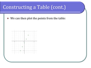
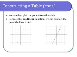
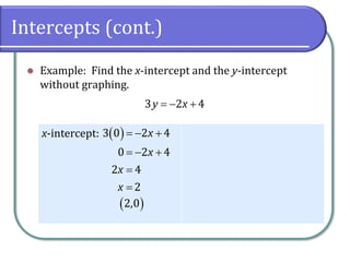
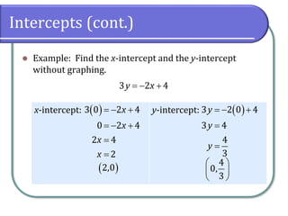
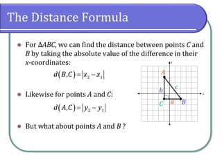
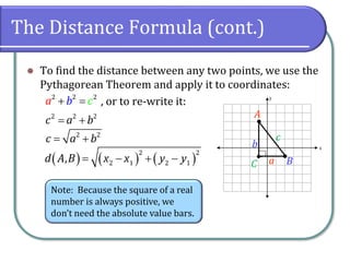
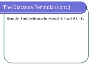
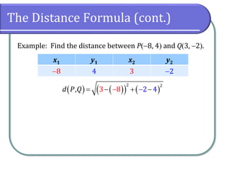
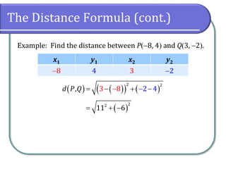
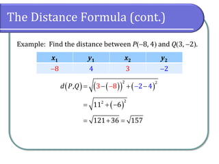
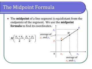
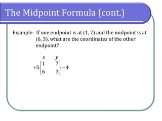
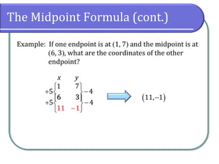
* Plot ordered pairs in a Cartesian coordinate system. * Graph equations by plotting points. * Find x-intercepts and y-intercepts. * Use the distance formula. * Use the midpoint formula.

1. 2.1 Rectangular Coordinates
Chapter 2 Equations and Inequalities

2. Concepts & Objectives
⚫ Objectives for this section:
⚫ Plot ordered pairs in a Cartesian coordinate system.
⚫ Graph equations by plotting points.
⚫ Find x-intercepts and y-intercepts.
⚫ Use the distance formula.
⚫ Use the midpoint formula.

3. Ordered Pairs
⚫ An ordered pair represents a relationship between two
sets. The first item in the pair represents an element in
the first set, and the second item in the pair represents
an element in the second set. A relationship between the
sets can be used to determine which element is paired
with which.
⚫ An example of an ordered pair relationship is numerical
grades and letter grades, such as (85, B).

4. Rectangular Coordinate System
⚫ Every real number corresponds to a point on a number
line. This idea is extended to ordered pairs of real
numbers by using two perpendicular number lines, one
horizontal and one vertical, that intersect at their zero-
points, which is called the origin.
⚫ The horizontal line is called the x-axis, and the vertical
line is called the y-axis.
⚫ Starting at the origin, the positive numbers go right (x)
and up (y), which the negative number go left (x) and
down (y).

5. Rectangular Coordinate System
⚫ The x-axis and y-axis together make up a rectangular
coordinate system, or Cartesian coordinate system
(named for one of its co-inventors, René Descartes; the
other was Pierre de Fermat).
⚫ The plane into which the coordinate
system is introduced is the coordinate
plane, or xy-plane. The x-axis and
y-axis divide the plane into four regions,
or quadrants; the points on the axes do
not belong to a quadrant.

6. Rectangular Coordinate System
⚫ Each point P in the xy-plane corresponds to a unique
ordered pair (a, b) of real numbers. The numbers a and
b are the coordinates of point P.
⚫ To locate the point corres-
ponding to the ordered pair
(3, −1), for example, start at the
origin, move 3 units in the
positive x-direction (right), then
move 1 unit in the negative
y-direction (down).

7. Constructing a Table of Values
⚫ Suppose we want to graph the equation y = 2x ‒ 1. We
can begin by substituting a value for x into the equation
and determining the resulting value of y. Each pair of x-
and y-values is an ordered pair that can plotted.
x y = 2x ‒ 1 (x, y)
‒2 y = 2(‒2)‒1 = ‒5 (‒2, ‒5)
‒1 y = 2(‒1)‒1 = ‒3 (‒1, ‒3)
0 y = 2(0)‒1 = ‒1 (0, ‒1)
1 y = 2(1)‒1 = 1 (1, 1)
2 y = 2(2)‒1 = 3 (2, 3)

8. Constructing a Table (cont.)
⚫ We can then plot the points from the table:

9. Constructing a Table (cont.)
⚫ We can then plot the points from the table:
⚫ Because this is a linear equation, we can connect the
points to form a line:

10. Intercepts
⚫ The intercepts of a graph are points at which the graph
crosses the axes.
⚫ The x-intercept is the point at which the graph
crosses the x-axis. At this point, the y-coordinate is 0.
⚫ The y-intercept is the point at which the graph
crosses the y-axis; therefore, the x-coordinate is 0.
⚫ To determine the x-intercept, we set y equal to zero and
solve for x. Similarly, to determine the y-intercept, we
set x equal to zero and solve for y.

11. Intercepts (cont.)
⚫ Example: Find the x-intercept and the y-intercept
without graphing.
3 2 4
y x
= − +

12. Intercepts (cont.)
x-intercept:
⚫ Example: Find the x-intercept and the y-intercept
without graphing.
3 2 4
y x
= − +
( )
3 0 2 4
0 2 4
2 4
2
x
x
x
x
= − +
= − +
=
=
( )
2,0

13. Intercepts (cont.)
x-intercept: y-intercept:
⚫ Example: Find the x-intercept and the y-intercept
without graphing.
3 2 4
y x
= − +
( )
3 0 2 4
0 2 4
2 4
2
x
x
x
x
= − +
= − +
=
=
( )
3 2 0 4
3 4
4
3
y
y
y
= − +
=
=
( )
2,0
4
0,
3
 
 
 

14. The Distance Formula
⚫ For ΔABC, we can find the distance between points C and
B by taking the absolute value of the difference in their
x-coordinates:
⚫ Likewise for points A and C:
⚫ But what about points A and B ?
y
x
a
b c
●
●
A
B
C
( )= −
2 1
,
d B C x x
( ) 2 1
,
d A C y y
= −

15. The Distance Formula (cont.)
⚫ To find the distance between any two points, we use the
Pythagorean Theorem and apply it to coordinates:
, or to re-write it: y
x
a
b
c
●
●
A
B
C
2 2 2
a c
b
+ =
2 2 2
c a b
= +
2 2
c a b
= +
( ) ( ) ( )
2 2
2 1 2 1
,
d A B x x y y
= − + −
Note: Because the square of a real
number is always positive, we
don’t need the absolute value bars.

16. The Distance Formula (cont.)
Example: Find the distance between P(−8, 4) and Q(3, −2).

17. The Distance Formula (cont.)
Example: Find the distance between P(−8, 4) and Q(3, −2).
( ) ( )
( ) ( )
2 2
3 8 2
, 4
d P Q = −
−
− + −
x1 y1 x2 y2
−8 4 3 −2

18. The Distance Formula (cont.)
Example: Find the distance between P(−8, 4) and Q(3, −2).
( ) ( )
( ) ( )
2 2
3 8 2
, 4
d P Q = −
−
− + −
x1 y1 x2 y2
−8 4 3 −2
( )
2
2
11 6
= + −

19. The Distance Formula (cont.)
Example: Find the distance between P(−8, 4) and Q(3, −2).
( ) ( )
( ) ( )
2 2
3 8 2
, 4
d P Q = −
−
− + −
x1 y1 x2 y2
−8 4 3 −2
( )
2
2
11 6
= + −
121 36 157
= + =

20. The Midpoint Formula
⚫ The midpoint of a line segment is equidistant from the
endpoints of the segment. We use the midpoint
formula to find its coordinates.
0
A
B
x1 x2
y1
y2
●
M
average of
x1 and x2
average of
y1 and y2
1 2 1 2
,
2 2
x x y y
M
+ +
 
 
 

21. The Midpoint Formula (cont.)
Example: Find the coordinates of the midpoint M of the
segment with endpoints (8, −4) and (−6, 1).

22. The Midpoint Formula (cont.)
Example: Find the coordinates of the midpoint M of the
segment with endpoints (8, −4) and (−6, 1).
( )
8 6 4 1
,
2 2
M
 
+ − − +
 
 
3
1,
2
M
 
= −
 
 

23. The Midpoint Formula (cont.)
⚫ If you are given an endpoint and a midpoint, you will
then need to find the other endpoint. While you can use
the midpoint formula and Algebra to find the missing
coordinates, I find it much easier to take advantage of
the definition – the distance between each should be the
same.
⚫ Line up the points and find the amount that is being
added or subtracted to produce the midpoint. Then add
or subtract that same amount to produce the other
endpoint.

24. The Midpoint Formula (cont.)
Example: If one endpoint is at (1, 7) and the midpoint is at
(6, 3), what are the coordinates of the other
endpoint?

25. The Midpoint Formula (cont.)
Example: If one endpoint is at (1, 7) and the midpoint is at
(6, 3), what are the coordinates of the other
endpoint?
1 7
5 4
6 3
 
+ −
 
 
x y

26. The Midpoint Formula (cont.)
Example: If one endpoint is at (1, 7) and the midpoint is at
(6, 3), what are the coordinates of the other
endpoint?
1 7
5 4
6 3
 
+ −
 
 
 
+ −

 
−

6 3
5 4
1
11
( )
11, 1
−
x y

27. Classwork
⚫ College Algebra 2e
⚫ 2.1: 6-16 (even); 1.6: 16-32 (×4); 1.5: 38-50 (even)
⚫ 2.1 Classwork Check
⚫ Quiz 1.6