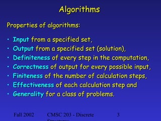
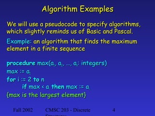
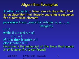
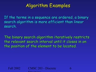
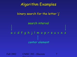
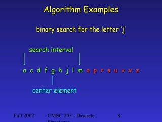
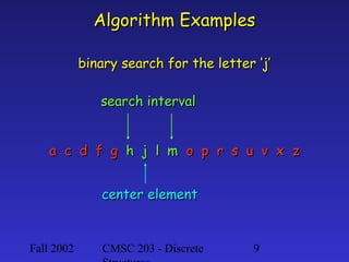
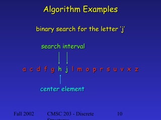
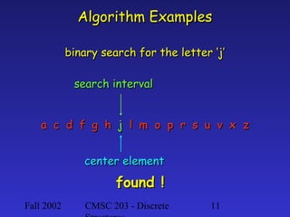
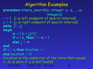
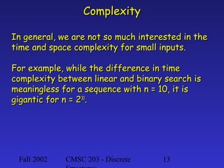
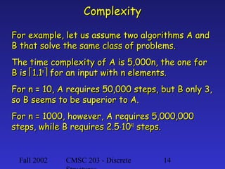
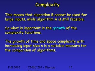
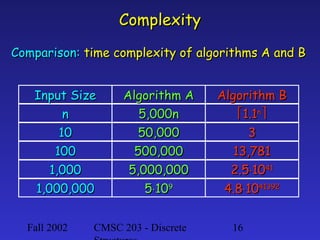
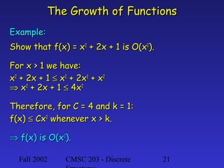
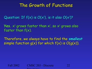
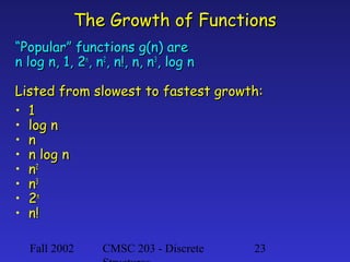
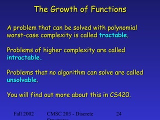
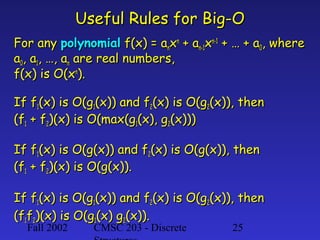
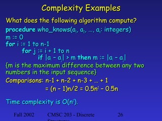
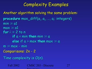
This document introduces algorithms and their properties. It defines an algorithm as a precise set of instructions to perform a computation or solve a problem. Key properties of algorithms are discussed such as inputs, outputs, definiteness, correctness, finiteness, effectiveness and generality. Examples are given of maximum finding, linear search and binary search algorithms using pseudocode. The document discusses how algorithm complexity grows with input size and introduces big-O notation to analyze asymptotic growth rates of algorithms. It provides examples of analyzing time complexities for different algorithms.

1. Enough Mathematical Appetizers!
Let us look at something more interesting:
Algorithms
Fall 2002
CMSC 203 - Discrete
1

2. Algorithms
What is an algorithm?
An algorithm is a finite set of precise instructions
for performing a computation or for solving a
problem.
This is a rather vague definition. You will get to
know a more precise and mathematically useful
definition when you attend CS420.
But this one is good enough for now…
Fall 2002
CMSC 203 - Discrete
2

3. Algorithms
Properties of algorithms:
•
•
•
•
•
•
•
Input from a specified set,
Output from a specified set (solution),
Definiteness of every step in the computation,
Correctness of output for every possible input,
Finiteness of the number of calculation steps,
Effectiveness of each calculation step and
Generality for a class of problems.
Fall 2002
CMSC 203 - Discrete
3

4. Algorithm Examples
We will use a pseudocode to specify algorithms,
which slightly reminds us of Basic and Pascal.
Example: an algorithm that finds the maximum
element in a finite sequence
procedure max(a1, a2, …, an: integers)
max := a1
for i := 2 to n
if max < ai then max := ai
{max is the largest element}
Fall 2002
CMSC 203 - Discrete
4

5. Algorithm Examples
Another example: a linear search algorithm, that
is, an algorithm that linearly searches a sequence
for a particular element.
procedure linear_search(x: integer; a1, a2, …, an:
integers)
i := 1
while (i ≤ n and x ≠ ai)
i := i + 1
if i ≤ n then location := i
else location := 0
{location is the subscript of the term that equals
x, or is zero if x is not found}
Fall 2002
CMSC 203 - Discrete
5

6. Algorithm Examples
If the terms in a sequence are ordered, a binary
search algorithm is more efficient than linear
search.
The binary search algorithm iteratively restricts
the relevant search interval until it closes in on
the position of the element to be located.
Fall 2002
CMSC 203 - Discrete
6

7. Algorithm Examples
binary search for the letter ‘j’
search interval
a c d f g h j l m o p r s u v x z
center element
Fall 2002
CMSC 203 - Discrete
7

8. Algorithm Examples
binary search for the letter ‘j’
search interval
a c d f g h j l m o p r s u v x z
center element
Fall 2002
CMSC 203 - Discrete
8

9. Algorithm Examples
binary search for the letter ‘j’
search interval
a c d f g h j l m o p r s u v x z
center element
Fall 2002
CMSC 203 - Discrete
9

10. Algorithm Examples
binary search for the letter ‘j’
search interval
a c d f g h j l m o p r s u v x z
center element
Fall 2002
CMSC 203 - Discrete
10

11. Algorithm Examples
binary search for the letter ‘j’
search interval
a c d f g h j l m o p r s u v x z
center element
found !
Fall 2002
CMSC 203 - Discrete
11

12. Algorithm Examples
procedure binary_search(x: integer; a1, a2, …, an:
integers)
i := 1 {i is left endpoint of search interval}
j := n {j is right endpoint of search interval}
while (i < j)
begin
m := (i + j)/2
if x > am then i := m + 1
else j := m
end
if x = ai then location := i
else location := 0
{location is the subscript of the term that equals
x, or is zero if x is not found}
Fall 2002
CMSC 203 - Discrete
12

13. Complexity
In general, we are not so much interested in the
time and space complexity for small inputs.
For example, while the difference in time
complexity between linear and binary search is
meaningless for a sequence with n = 10, it is
gigantic for n = 230.
Fall 2002
CMSC 203 - Discrete
13

14. Complexity
For example, let us assume two algorithms A and
B that solve the same class of problems.
The time complexity of A is 5,000n, the one for
B is 1.1n for an input with n elements.
For n = 10, A requires 50,000 steps, but B only 3,
so B seems to be superior to A.
For n = 1000, however, A requires 5,000,000
steps, while B requires 2.5⋅1041 steps.
Fall 2002
CMSC 203 - Discrete
14

15. Complexity
This means that algorithm B cannot be used for
large inputs, while algorithm A is still feasible.
So what is important is the growth of the
complexity functions.
The growth of time and space complexity with
increasing input size n is a suitable measure for
the comparison of algorithms.
Fall 2002
CMSC 203 - Discrete
15

16. Complexity
Comparison: time complexity of algorithms A and B
Input Size
n
10
100
1,000
1,000,000
Fall 2002
Algorithm A
5,000n
50,000
500,000
5,000,000
5⋅109
CMSC 203 - Discrete
Algorithm B
1.1n
3
13,781
2.5⋅1041
4.8⋅1041392
16

17. Complexity
This means that algorithm B cannot be used for
large inputs, while running algorithm A is still
feasible.
So what is important is the growth of the
complexity functions.
The growth of time and space complexity with
increasing input size n is a suitable measure for
the comparison of algorithms.
Fall 2002
CMSC 203 - Discrete
17

18. The Growth of Functions
The growth of functions is usually described
using the big-O notation.
Definition: Let f and g be functions from the
integers or the real numbers to the real numbers.
We say that f(x) is O(g(x)) if there are constants
C and k such that
|f(x)| ≤ C|g(x)|
whenever x > k.
Fall 2002
CMSC 203 - Discrete
18

19. The Growth of Functions
When we analyze the growth of complexity
functions, f(x) and g(x) are always positive.
Therefore, we can simplify the big-O requirement
to
f(x) ≤ C⋅g(x) whenever x > k.
If we want to show that f(x) is O(g(x)), we only
need to find one pair (C, k) (which is never unique).
Fall 2002
CMSC 203 - Discrete
19

20. The Growth of Functions
The idea behind the big-O notation is to establish
an upper boundary for the growth of a function
f(x) for large x.
This boundary is specified by a function g(x) that
is usually much simpler than f(x).
We accept the constant C in the requirement
f(x) ≤ C⋅g(x) whenever x > k,
because C does not grow with x.
We are only interested in large x, so it is OK if
f(x) > C⋅g(x) for x ≤ k.
Fall 2002
CMSC 203 - Discrete
20

21. The Growth of Functions
Example:
Show that f(x) = x2 + 2x + 1 is O(x2).
For x > 1 we have:
x2 + 2x + 1 ≤ x2 + 2x2 + x2
⇒ x2 + 2x + 1 ≤ 4x2
Therefore, for C = 4 and k = 1:
f(x) ≤ Cx2 whenever x > k.
⇒ f(x) is O(x2).
Fall 2002
CMSC 203 - Discrete
21

22. The Growth of Functions
Question: If f(x) is O(x2), is it also O(x3)?
Yes. x3 grows faster than x2, so x3 grows also
faster than f(x).
Therefore, we always have to find the smallest
simple function g(x) for which f(x) is O(g(x)).
Fall 2002
CMSC 203 - Discrete
22

23. The Growth of Functions
“Popular” functions g(n) are
n log n, 1, 2n, n2, n!, n, n3, log n
Listed from slowest to fastest growth:
• 1
• log n
• n
• n log n
• n2
• n3
• 2n
• n!
Fall 2002
CMSC 203 - Discrete
23

24. The Growth of Functions
A problem that can be solved with polynomial
worst-case complexity is called tractable.
Problems of higher complexity are called
intractable.
Problems that no algorithm can solve are called
unsolvable.
You will find out more about this in CS420.
Fall 2002
CMSC 203 - Discrete
24

25. Useful Rules for Big-O
For any polynomial f(x) = anxn + an-1xn-1 + … + a0, where
a0, a1, …, an are real numbers,
f(x) is O(xn).
If f1(x) is O(g1(x)) and f2(x) is O(g2(x)), then
(f1 + f2)(x) is O(max(g1(x), g2(x)))
If f1(x) is O(g(x)) and f2(x) is O(g(x)), then
(f1 + f2)(x) is O(g(x)).
If f1(x) is O(g1(x)) and f2(x) is O(g2(x)), then
(f1f2)(x) is O(g1(x) g2(x)).
Fall 2002
CMSC 203 - Discrete
25

26. Complexity Examples
What does the following algorithm compute?
procedure who_knows(a1, a2, …, an: integers)
m := 0
for i := 1 to n-1
for j := i + 1 to n
if |ai – aj| > m then m := |ai – aj|
{m is the maximum difference between any two
numbers in the input sequence}
Comparisons: n-1 + n-2 + n-3 + … + 1
= (n – 1)n/2 = 0.5n2 – 0.5n
Time complexity is O(n2).
Fall 2002
CMSC 203 - Discrete
26

27. Complexity Examples
Another algorithm solving the same problem:
procedure max_diff(a1, a2, …, an: integers)
min := a1
max := a1
for i := 2 to n
if ai < min then min := ai
else if ai > max then max := ai
m := max - min
Comparisons: 2n - 2
Time complexity is O(n).
Fall 2002
CMSC 203 - Discrete
27