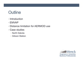
The document presents air dispersion modeling highlights shared during the 2012 A&WMA UMS Board Meeting, focusing on the use of models like AERMOD for predicting air quality and its limitations. It discusses various case studies, including air quality assessments in North Dakota and the Gibson generating station, emphasizing modeling challenges and the importance of accurate emission variability processing. The findings indicate significant variability in modeled results based on emission rates and the appropriateness of distance limitations in dispersion models.

1. AIR DISPERSION
MODELING HIGHLIGHTS
FROM 2012 ACE
Presentation for the A&WMA UMS Board Meeting
August 21, 2012
Sergio Guerra
Wenck Associates, Inc.

2. Outline
• Introduction
• EMVAP
• Distance limitation for AERMOD use
• Case studies
• North Dakota
• Gibson Station

3. Why do we use a model?

4. What is a model?
• A Model is a way of expressing the
relationship between the different variables
of a system in mathematical terms

5. What is an Air Quality Model
An
attempt to predict or simulate the ambient
concentrations of contaminants in an area of interest.
An Air Quality Model can be as simple as an algebraic
equation or more complex

6. AERMOD
• AERMOD is a steady-state plume model that incorporates
air dispersion based on planetary boundary layer
turbulence structure and scaling concepts, including
treatment of both surface and elevated sources, and both
simple and complex terrain.
• AERMOD replaced the Industrial Source Complex
(ISCST3) model as EPA’s regulatory model on December
9, 2006
• Preprocessors include:
AERMET,AERMINUTE,AERSURFACE,AERMAP,BPIP

7. What are the inputs of a dispersion
model?
• Source data
• Building data
• Receptor data
• Site data
• Meteorological data
• Terrain data

8. ACE 2012 Highlights

9. Emissions Variability Processor (EMVAP)
EMVAP an Emission Variability Processor for Modeling
Applications
Paper 2012-A-341-AWMA
Richard P. Hamel, Robert J. Paine, David W. Heinold (AECOM)
Naresh Kumar and Eladio Knipping (EPRI)

10. EMVAP
• Large variation possible over the course of a year
• Intermittent sources (e.g., emergency backup engines or
bypass stacks) present modeling challenges
• For these sources, assuming fixed peak 1‐hour emissions
on a continuous basis will result in unrealistic modeled
results
• Better approach is to assume a prescribed distribution of
emission rates
• EMVAP uses this information to develop alternative ways
to indicate modeled compliance using a range of emission
rates instead of just one value

11. Hourly emission profile

12. Cumulative frequency distribution

20. Distance limitations of AERMOD
Limitations of Steady-State Dispersion Models and
Possible Advanced Approaches
Paper 2012-500-AWMA
Gary Moore, Robert Paine, and David Heinold (AECOM)
Steve Hanna (Hanna Consultants)

21. Short range model distance applicability
• Plumes are assumed to travel to infinite distances within 1
•
•
•
•
hour (“lighthouse beam” effect)
Each hour, the previous hour’s emissions are replaced
and forgotten
Worst‐case conditions, especially associated with low
winds, result in impossible distances
Currently, though, US EPA considers these models to be
applicable to a rather arbitrary distance of 50 km
Equivalence between ISC and CALPUFF for 2 met data
locations:
• Salem, Oregon
• Evansville, Indiana

26. Short range model distance applicability
• 20‐30 km is the extent a single hour’s travel for most of
the hours
• Even after 4‐5 hours, more than half of air parcels
followed with a 10‐m wind are still on the 50‐km modeling
domain
• Results suggest that a 20‐km limit seems more
appropriate for steady‐state model (e.g., AERMOD)
applicability rather than the current limit of 50 km

27. Case Study 1- North Dakota
Comparison of AERMOD Modeled 1-hour SO2
Concentrations to Observations at Multiple Monitoring
Stations in North Dakota
Paper 2012-A-353-AWMA
Mary M. Kaplan, Robert Paine (AECOM)

28. Evaluation Opportunity in North Dakota
• Mercer County: Antelope Valley Station and Great Plains
•
•
•
•
•
Synfuels Plant
Electrical generating unit sources dominate SO2
emissions – hourly data available
Five SO2 monitors in area within about 10 km of two
nearby “central” sources
Site‐specific PSD quality meteorological data years
available (10‐m tower)
Major SO2 sources within 50 km were modeled
Five recent years of data were used

30. Case Study 1- Dakota Gasification Co.
• Allowable emissions used for all sources, assumed to be
constantly at peak rates
• Receptors placed at monitor sites only, using actual
terrain (even though slopes are < 2%), except to
characterize the spatial concentration pattern
• Four of the five monitors were at elevations near local
stack base, a fifth monitor was about 100 m higher

33. Test of Terrain Problem for Gentle Slope
• Used generic tall stack buoyant source
• Modeled both flat and very gentle terrain
• Terrain case was uniformly sloped upward 1% in all
directions
• Modeled entire year of meteorology
• Obtained peak concentration on each ring of receptors
out to 50 km
• Plots follow for flat and gently sloping terrain

35. Conclusions from Gentle Slope Test
• AERMOD has unusual prediction result for very low wind,
•
•
•
•
stable conditions and low slope
Problem is, in part, caused by very low mixing height that
leads to very compact plume
Mixing height is below building obstacles, which the
model does not know about
Plume stays perfectly level; terrain should not be
considered in these cases
With terrain, result is an unexpected plume impact “bulge”
at point of terrain impact

36. Case Study 2-Gibson Generating Station
• Review of IDEM’s AERMOD Evaluation for the Gibson
Generating Station
• Robert Paine and Carlos Szembek (AECOM)

37. Case Study 2-Gibson Generating Station
• The Indiana Department of Environmental Management
(IDEM) conducted an evaluation of AERMOD
• Gibson is an isolated source with 4 stacks and 3 nearby
monitors
• On-site met data and hourly SO2 emission data for 2010
• Comparison of monitored versus predicted concentrations

39. Case Study 2-Gibson Generating Station

40. Case Study 2-Gibson Generating Station
• Low winds produced highest concentrations (~0.5m/s)
• Plume travel distance within an hour is short of the
distance needed to reach maximum receptors
• Formulation problem or coding error related to sigma-z
(used to calculate effective mixing lid)

41. Questions?
Sergio A. Guerra
Environmental Engineer
Phone: (651) 395-5225
sguerra@wenck.com