CSA 3702 machine learning module 4

CSA 3702 – MACHINE LEARNING
PREPARED BY,
NANDHINI S (SRMIST, RAMAPURAM CAMPUS),
BHARATHI RAJA N, MENNAKSHI COLLEGE OF ENGINEERING.

Module - IV
Optimization Techniques

• Genetic algorithm reflects the process of natural selection where
the fittest individuals are selected for reproduction in order to
produce offspring of the next generation.
• Genetic algorithms are stochastic search algorithms which act on a
population of possible solutions.
• The potential solutions are encoded as ‘genes’ — strings of
characters from some alphabet.
• New solutions can be produced by ‘mutating’ members of the
current population, and by ‘mating’ two solutions together to form a
new solution.
• The better solutions are selected to breed and mutate and the worse
ones are discarded.

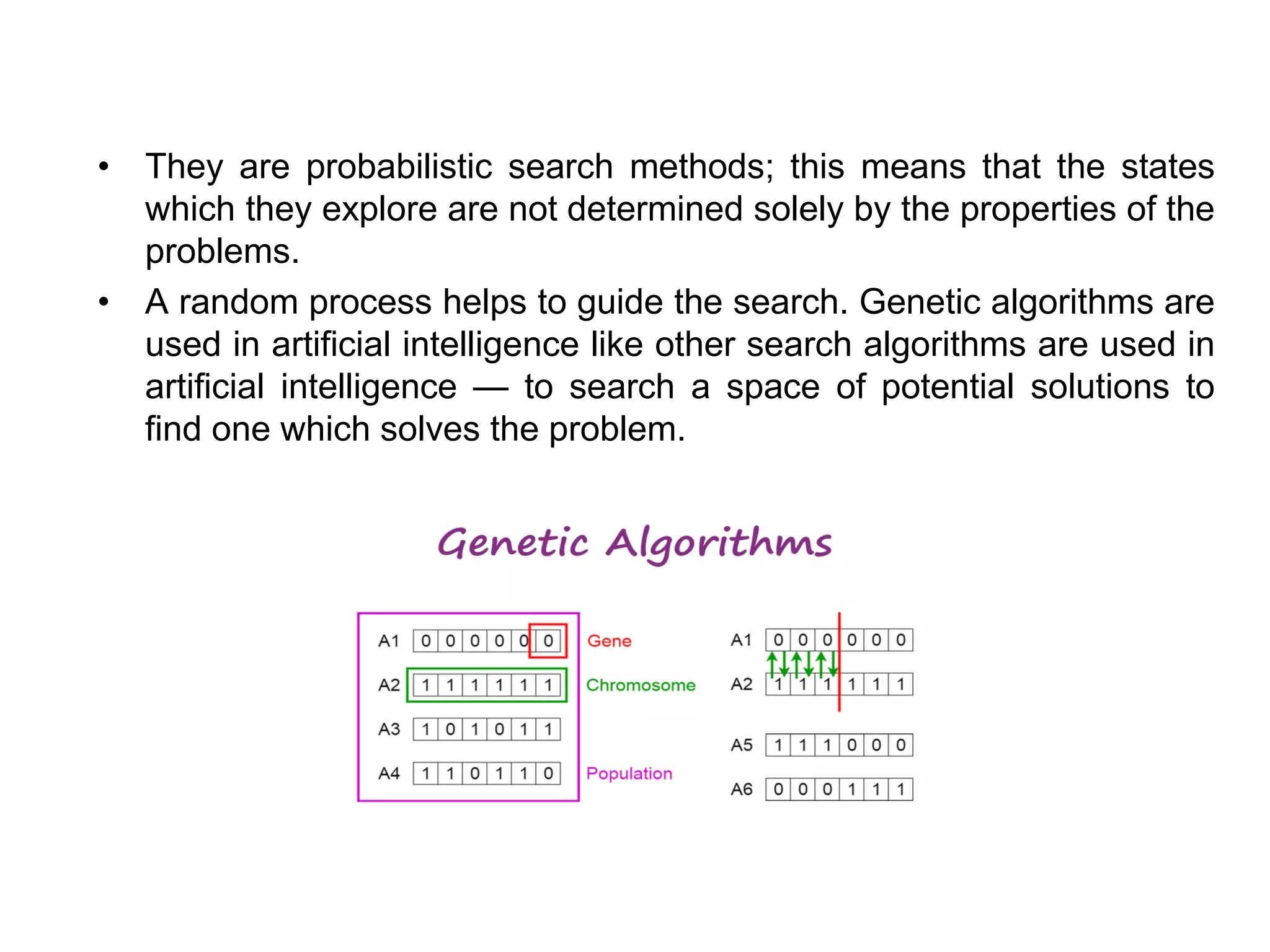
• They are probabilistic search methods; this means that the states
which they explore are not determined solely by the properties of the
problems.
• A random process helps to guide the search. Genetic algorithms are
used in artificial intelligence like other search algorithms are used in
artificial intelligence — to search a space of potential solutions to
find one which solves the problem.

Notion of Natural Selection
• The process of natural selection starts with the selection of fittest
individuals from a population. They produce offspring which inherit
the characteristics of the parents and will be added to the next
generation.
• If parents have better fitness, their offspring will be better than
parents and have a better chance at surviving. This process keeps
on iterating and at the end, a generation with the fittest individuals
will be found.
• This notion can be applied for a search problem. We consider a set
of solutions for a problem and select the set of best ones out of
them.

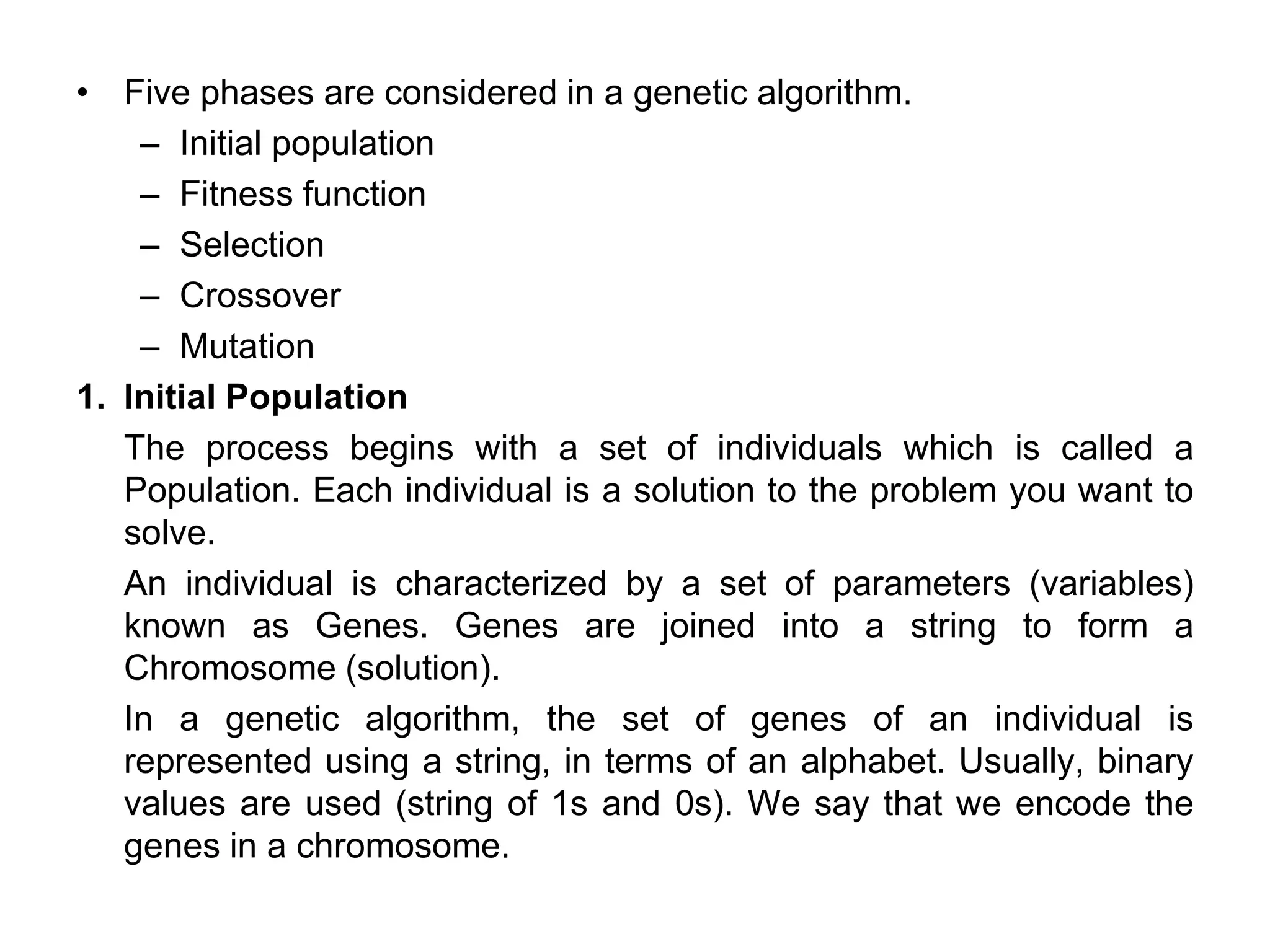
• Five phases are considered in a genetic algorithm.
– Initial population
– Fitness function
– Selection
– Crossover
– Mutation
1. Initial Population
The process begins with a set of individuals which is called a
Population. Each individual is a solution to the problem you want to
solve.
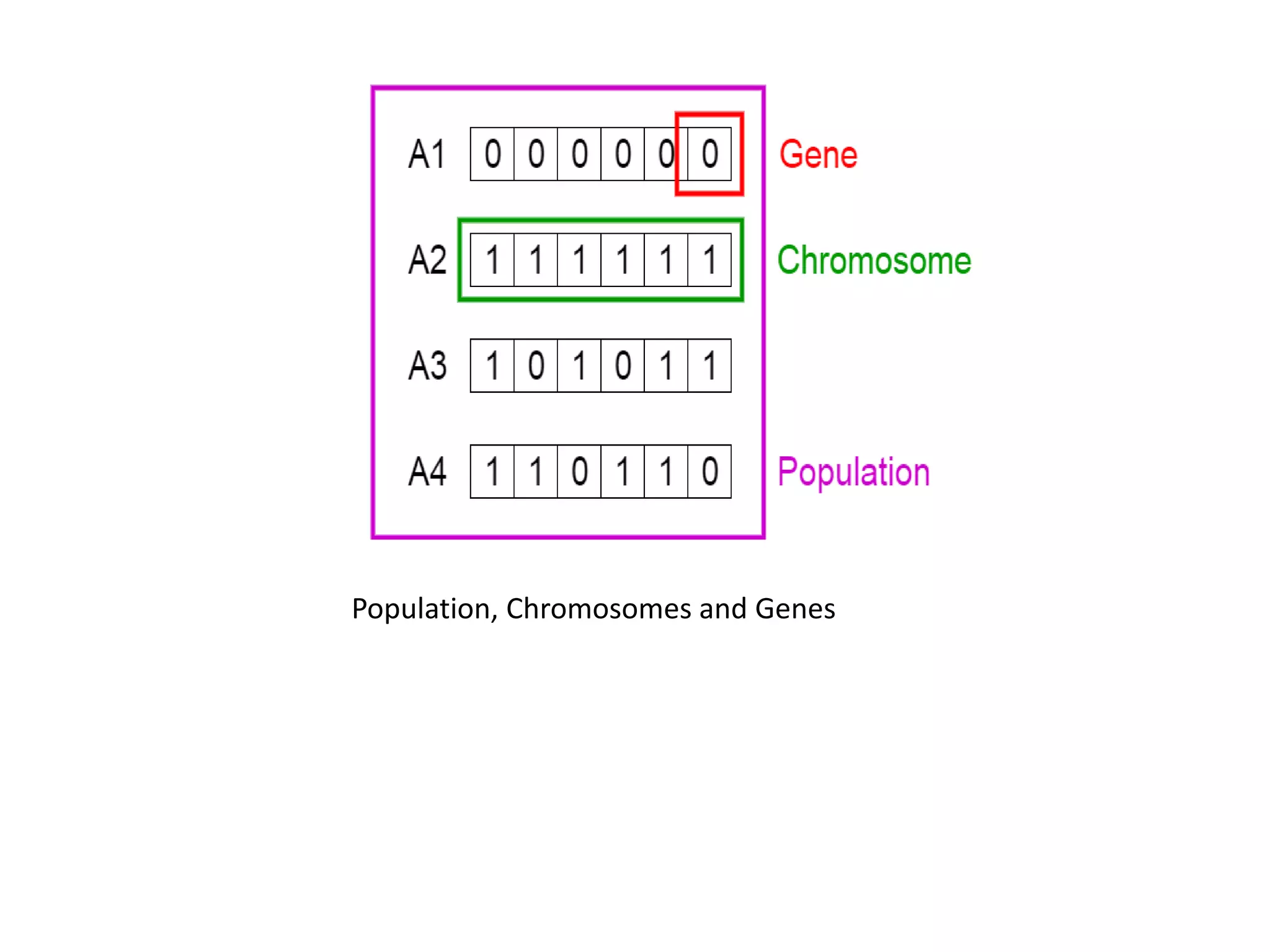
An individual is characterized by a set of parameters (variables)
known as Genes. Genes are joined into a string to form a
Chromosome (solution).
In a genetic algorithm, the set of genes of an individual is
represented using a string, in terms of an alphabet. Usually, binary
values are used (string of 1s and 0s). We say that we encode the
genes in a chromosome.

Population, Chromosomes and Genes

2. Fitness Function
• The fitness function determines how fit an individual is (the ability
of an individual to compete with other individuals).
• It gives a fitness score to each individual. The probability that an
individual will be selected for reproduction is based on its fitness
score.
3. Selection
• The idea of selection phase is to select the fittest individuals and let
them pass their genes to the next generation.
• Two pairs of individuals (parents) are selected based on their
fitness scores.
• Individuals with high fitness have more chance to be selected for
reproduction.

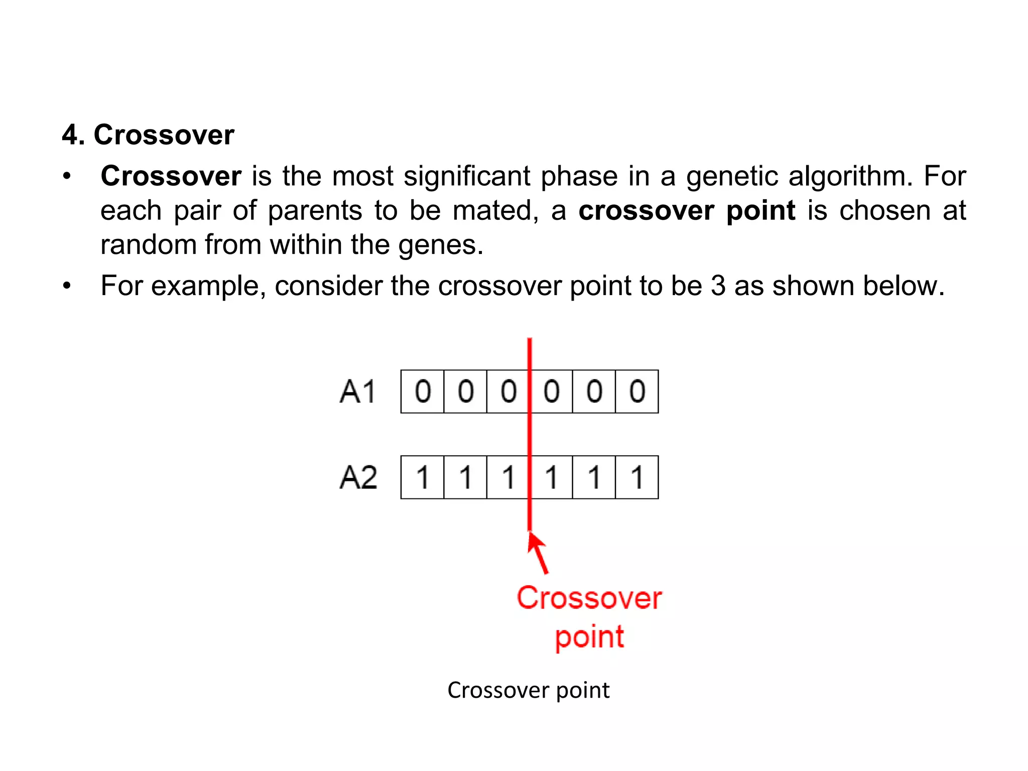
4. Crossover
• Crossover is the most significant phase in a genetic algorithm. For
each pair of parents to be mated, a crossover point is chosen at
random from within the genes.
• For example, consider the crossover point to be 3 as shown below.
Crossover point

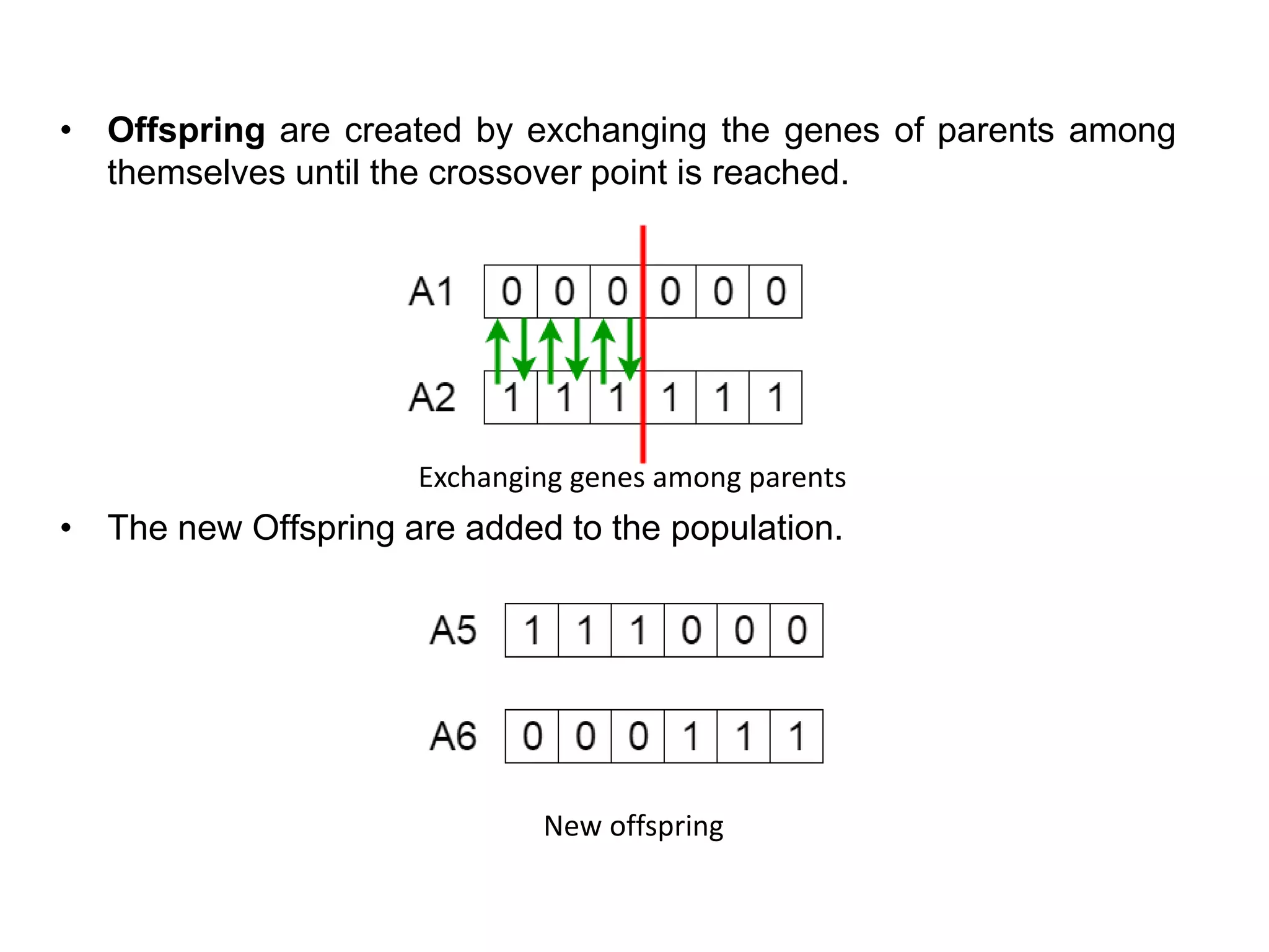
• Offspring are created by exchanging the genes of parents among
themselves until the crossover point is reached.
• The new Offspring are added to the population.
Exchanging genes among parents
New offspring

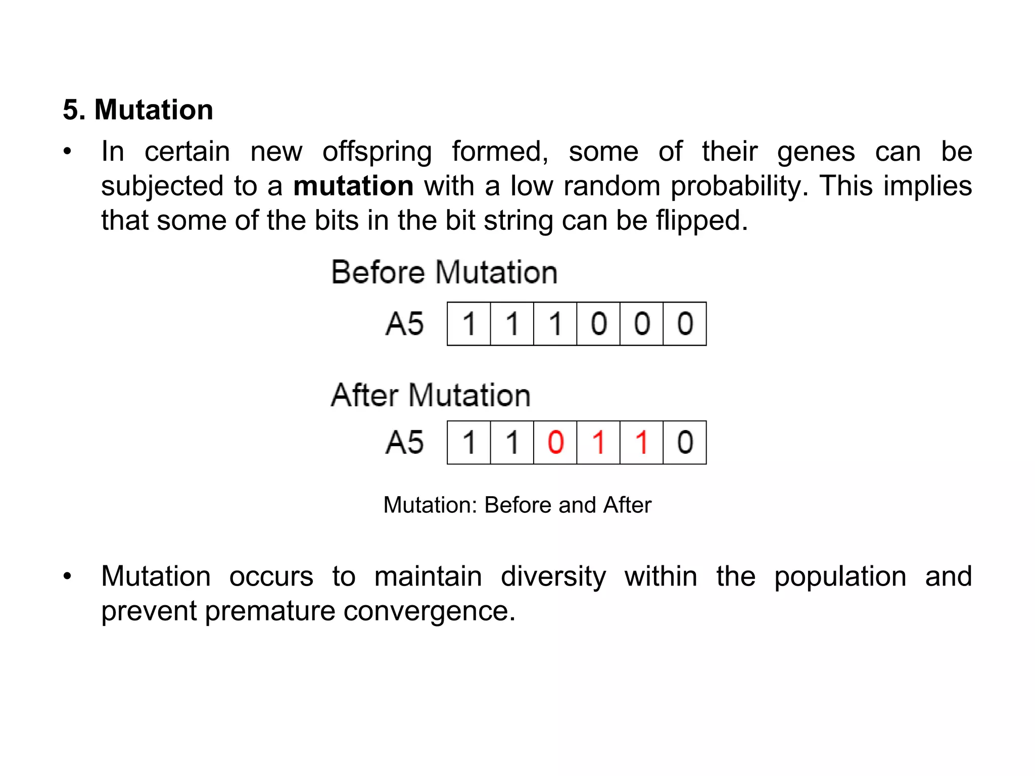
5. Mutation
• In certain new offspring formed, some of their genes can be
subjected to a mutation with a low random probability. This implies
that some of the bits in the bit string can be flipped.
Mutation: Before and After
• Mutation occurs to maintain diversity within the population and
prevent premature convergence.

6. Termination
• The algorithm terminates if the population has converged (does not
produce offspring which are significantly different from the previous
generation).
• Then it is said that the genetic algorithm has provided a set of
solutions to our problem.
Comments
• The population has a fixed size. As new generations are formed,
individuals with least fitness die, providing space for new offspring.
• The sequence of phases is repeated to produce individuals in each
new generation which are better than the previous generation.

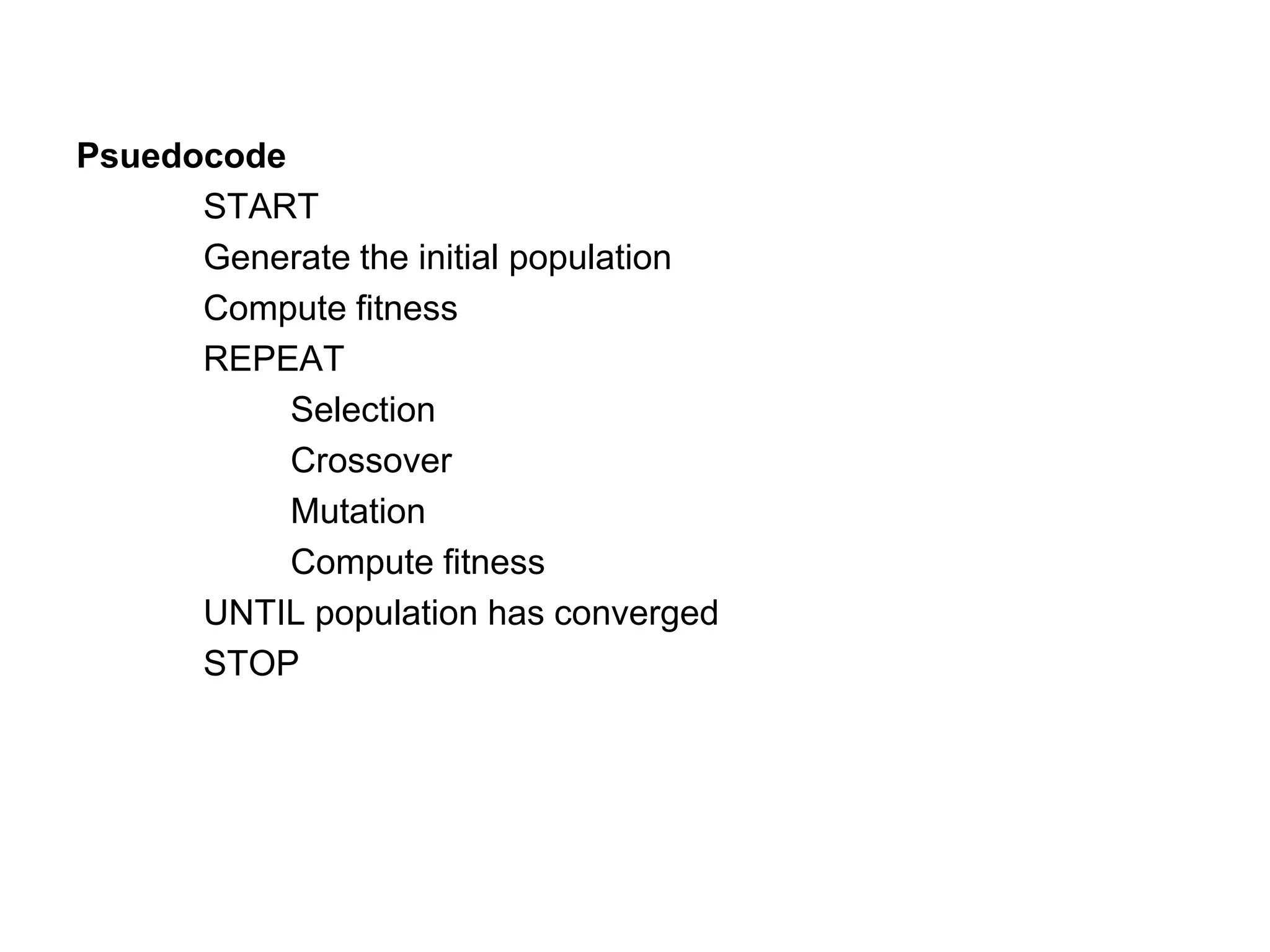
Psuedocode
START
Generate the initial population
Compute fitness
REPEAT
Selection
Crossover
Mutation
Compute fitness
UNTIL population has converged
STOP

• Genetic operator is a process used to maintain genetic diversity,
which is necessary for successful evolution.
• Genetic operators
Survival of the fittest (selection)
Reproduction (crossover)
Inheritance
Mutation
Selection
• selection operators give preference to better solutions
(chromosomes), allowing them to pass on their 'genes' to the next
generation of the algorithm.
• The best solutions are determined using some form of objective
function (also known as a 'fitness function' in genetic algorithms),
before being passed to the crossover operator.

• Crossover is a genetic operator used to vary the coding of
chromosomes from one generation to the next.
- Single-point Crossover
- Two-point Crossover
- Uniform Crossover
Single-point Crossover
• A crossover point on the parent chromosome is selected.
(Crossover mask defines the position of the crossover point.)
• All data beyond that point is swapped between two parents.
Two-point Crossover
• Two crossover point on the parent chromosome are selected. All
data between these points is swapped between two parents.
Uniform Crossover
• Crossover mask is generated as a random bit string. Bits are
sampled uniformly from the two parents.

• Inheritance is a genetic operator used to propagate problem solving
genes of fittest chromosomes to the next generation of evolved
solutions to the target problem.
• Mutation is a genetic operator used to maintain genetic diversity by
triggering small random changes in the bits of a chromosome.
• Procedure: A single bit is chosen at random and its value is
changed.
11100101011011 --------→11100100011011
• Purpose: Allow the algorithm to avoid local minima by preventing the
population of chromosomes from becoming too similar to each
other, thus slowing or even stopping evolution.
• Mutation rate: A percentage of the population to be mutated.

Combining operators
• While each operator acts to improve the solutions produced by the
genetic algorithm working individually, the operators must work in
conjunction with each other for the algorithm to be successful in
finding a good solution.
• Using the selection operator on its own will tend to fill the solution
population with copies of the best solution from the population.
• If the selection and crossover operators are used without the
mutation operator, the algorithm will tend to converge to a local
minimum, that is, a good but sub-optimal solution to the problem.
• Using the mutation operator on its own leads to a random
walk through the search space.
• Only by using all three operators together can the genetic algorithm
become a noise-tolerant hill-climbing algorithm, yielding good
solutions to the problem.

• Genetic Programming (GP) is a type of Evolutionary Algorithm
(EA), a subset of machine learning.
• EAs are used to discover solutions to problems humans do not know
how to solve, directly.
• Free of human preconceptions or biases, the adaptive nature of EAs
can generate solutions that are comparable to, and often better than
the best human efforts.
• GP can be used to discover a functional relationship between
features in data (symbolic regression), to group data into categories
(classification), and to assist in the design of electrical circuits,
antennae, and quantum algorithms.
• GP is applied to software engineering through code synthesis,
genetic improvement, automatic bug-fixing, and in developing game-
playing strategies.

Types of GP include
• Tree-based Genetic Programming
• Stack-based Genetic Programming
• Linear Genetic Programming (LGP)
• Grammatical Evolution
• Cartesian Genetic Programming (CGP)

Tree-based Genetic Programming
• Tree-based GP was the first application of Genetic Programming.
• In tree-based GP, the computer programs are represented in tree
structures that are evaluated recursively to produce the resulting
multivariate expressions.
• Traditional nomenclature states that a tree node (or just node) is an
operator [+,-,*,/] and a terminal node (or leaf) is a variable [a,b,c,d].
• Lisp was the first programming language applied to tree-based GP,
as the structure of this language matches the structure of the trees.
• However, many other languages such as Python, Java, and C++
have been used to develop tree-based GP applications.

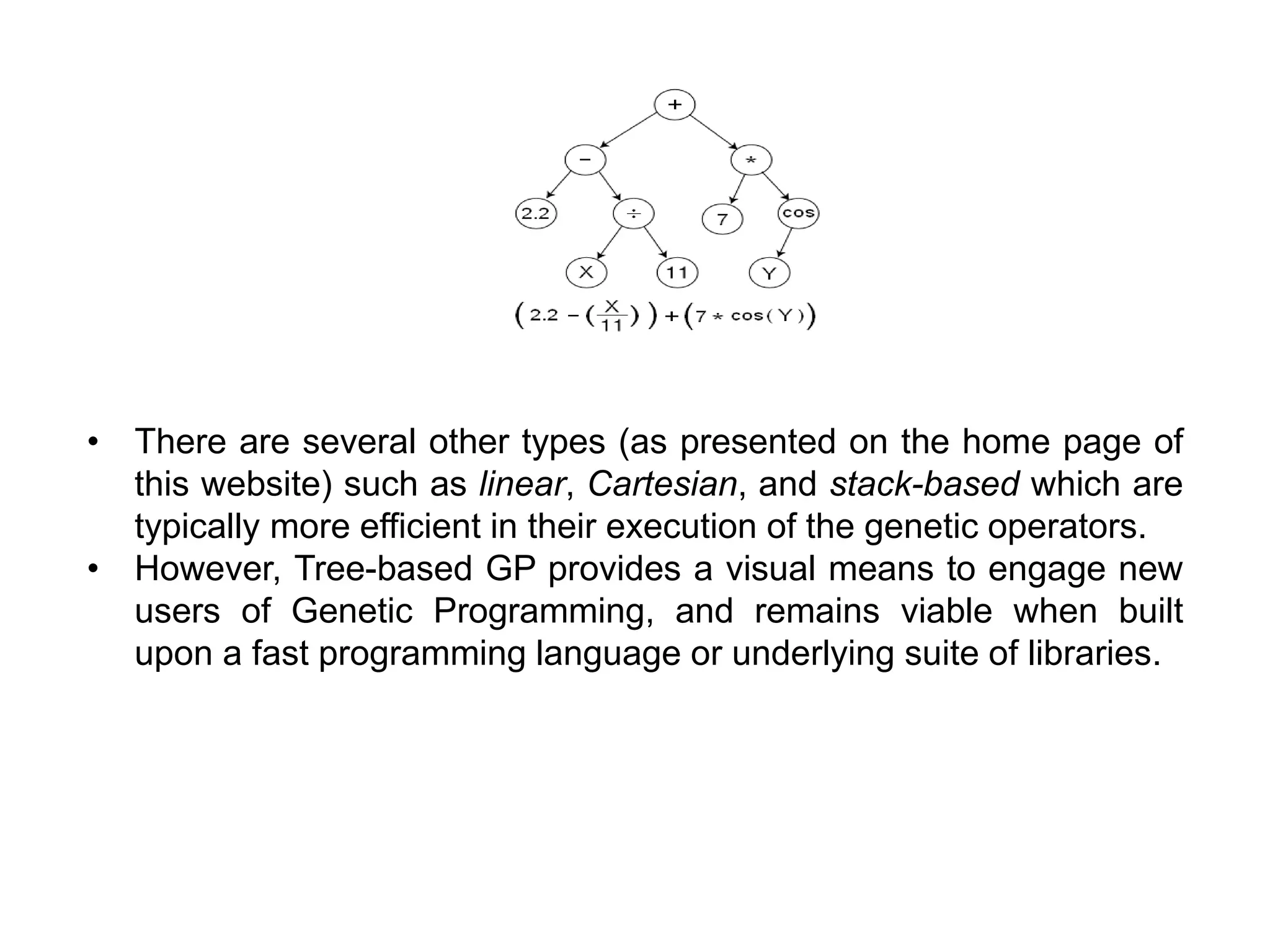
• There are several other types (as presented on the home page of
this website) such as linear, Cartesian, and stack-based which are
typically more efficient in their execution of the genetic operators.
• However, Tree-based GP provides a visual means to engage new
users of Genetic Programming, and remains viable when built
upon a fast programming language or underlying suite of libraries.

Linear genetic programming
• In genetic programming (GP) a linear tree is a program composed
of a variable number of unary functions and a single terminal.
• Linear genetic programming (LGP) is a particular subset of genetic
programming wherein computer programs in a population are
represented as a sequence of instructions from imperative
programming language or machine language.
• For example, a simple program written in the LGP language
below
input/ # gets an input from user and saves it to register F
0/ # sets register I = 0
save/ # saves content of F into data vector D[I] (i.e. D[0] := F)
input/ # gets another input, saves to F
add/ # adds to F current data pointed to by I (i.e. F := F +
D[0])
output/. # outputs result from F

Stack-based Genetic Programming
• In stack-based genetic programming, the programs in the evolving
population are expressed in a stack-based programming language.
• Was designed specifically for genetic programming, a separate
stack is provided for each data type, and program code itself can be
manipulated on data stacks and subsequently executed.
• Stack-based genetic programming can have a variety of advantages
over tree-based genetic programming.
• These may include improvements or simplifications to the handling
of multiple data types, bloat-free mutation and recombination
operators, execution tracing, programs with loops that provide valid
outputs even when terminated prematurely, parallelism, evolution of
arbitrary control structures, and automatic simplification of evolved
programs.

Cartesian genetic programming
• CGP is a highly efficient and flexible form of Genetic Programming
that encodes a graph representation of a computer program.
• CGP represents computational structures (mathematical equations,
circuits, computer programs etc) as a string of integers.
• These integers, known as genes determine the functions of nodes in
the graph, the connections between nodes, the connections to
inputs and the locations in the graph where outputs are taken from.
• Using a graph representation is very flexible as many computational
structures can be represented as graphs. A good example of this is
artificial neural networks (ANNs). These can be easily encoded in
CGP.

Grammatical Evolution
• The objective is to find an executable program or program fragment,
that will achieve a good fitness value for the given objective function.
• Grammatical Evolution applies genetic operators to an integer string,
subsequently mapped to a program (or similar) through the use of a
grammar.
• One of the benefits of GE is that this mapping simplifies the
application of search to different programming languages and other
structures.

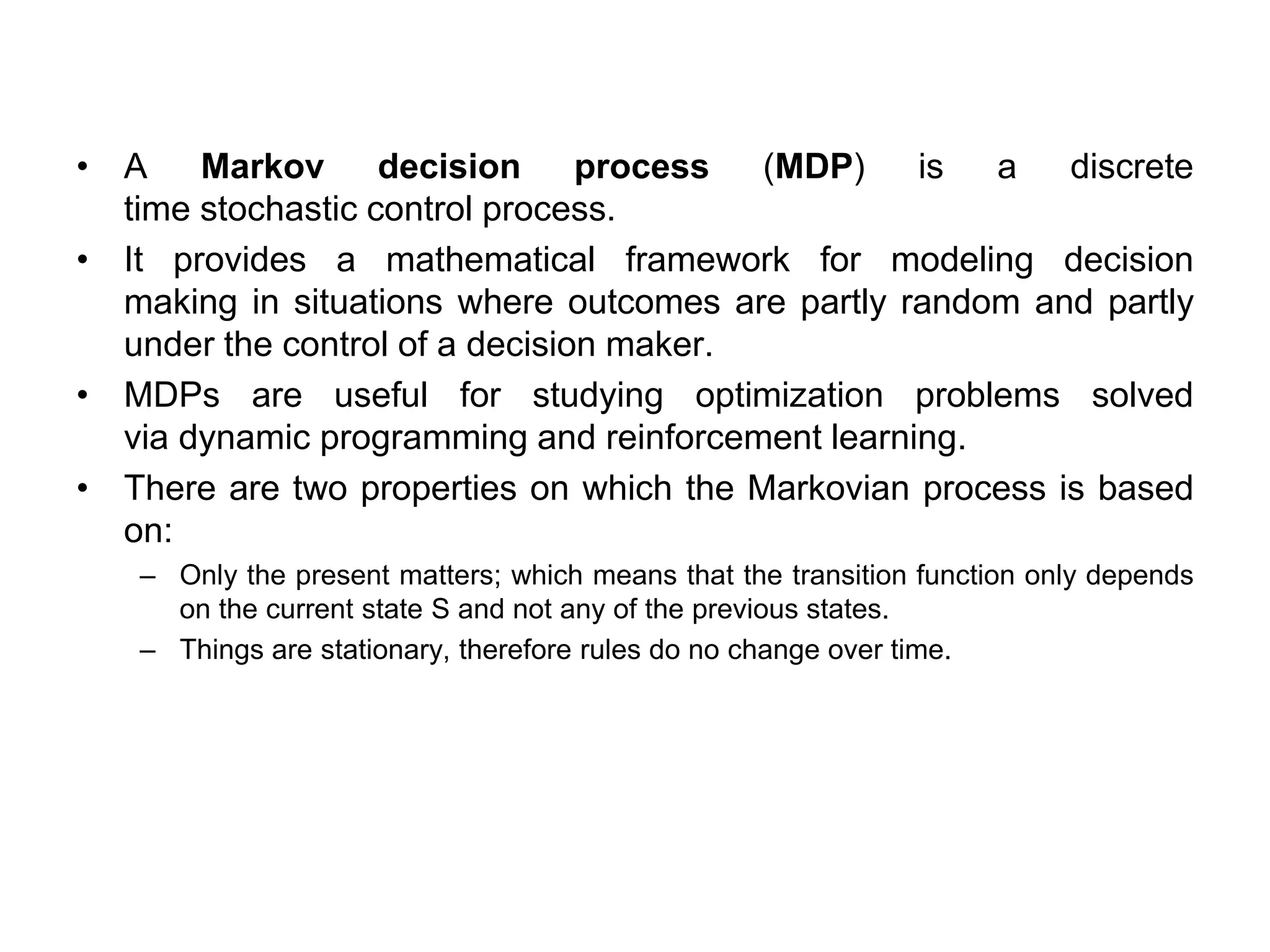
• A Markov decision process (MDP) is a discrete
time stochastic control process.
• It provides a mathematical framework for modeling decision
making in situations where outcomes are partly random and partly
under the control of a decision maker.
• MDPs are useful for studying optimization problems solved
via dynamic programming and reinforcement learning.
• There are two properties on which the Markovian process is based
on:
– Only the present matters; which means that the transition function only depends
on the current state S and not any of the previous states.
– Things are stationary, therefore rules do no change over time.

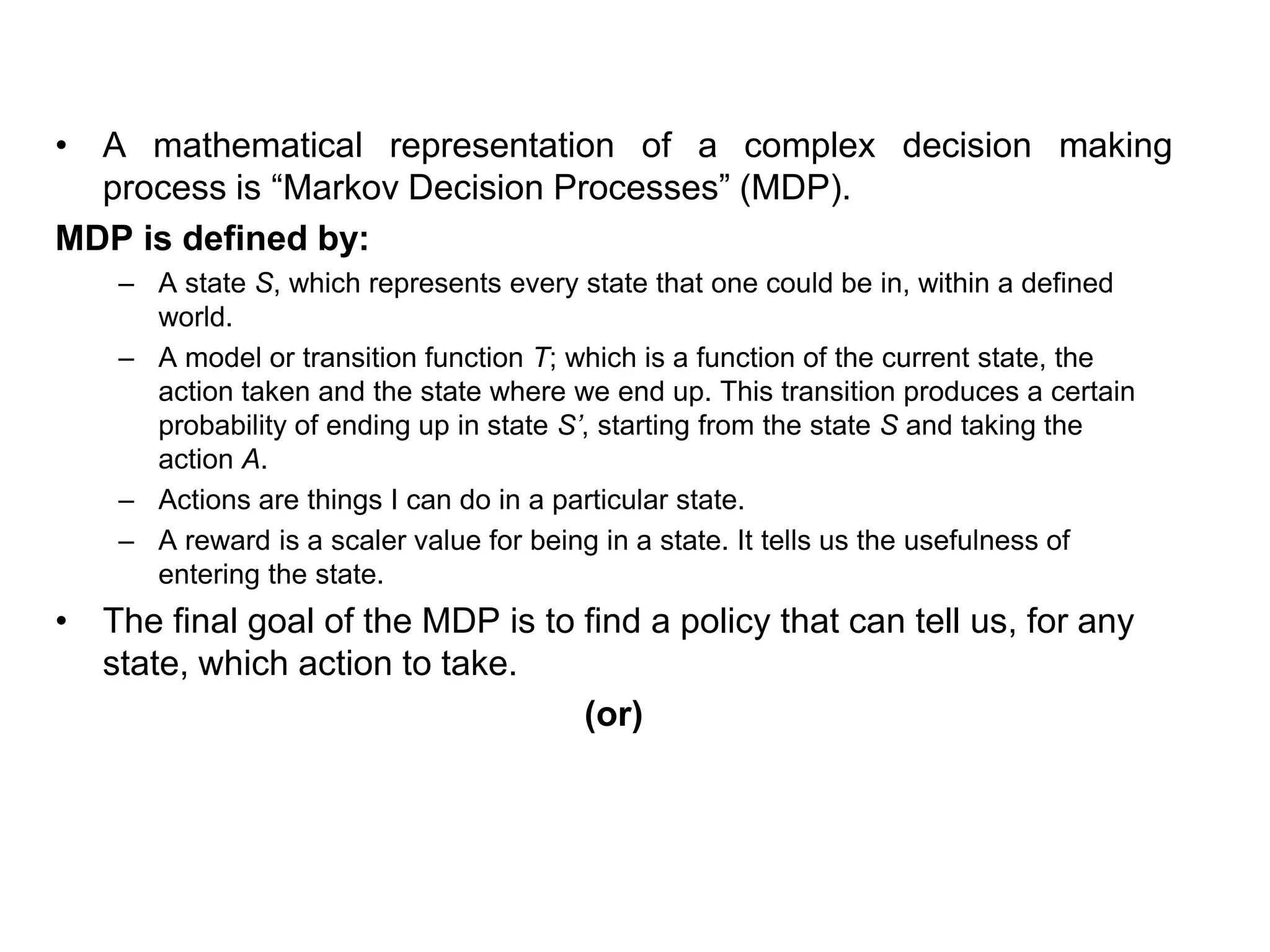
• A mathematical representation of a complex decision making
process is “Markov Decision Processes” (MDP).
MDP is defined by:
– A state S, which represents every state that one could be in, within a defined
world.
– A model or transition function T; which is a function of the current state, the
action taken and the state where we end up. This transition produces a certain
probability of ending up in state S’, starting from the state S and taking the
action A.
– Actions are things I can do in a particular state.
– A reward is a scaler value for being in a state. It tells us the usefulness of
entering the state.
• The final goal of the MDP is to find a policy that can tell us, for any
state, which action to take.
(or)

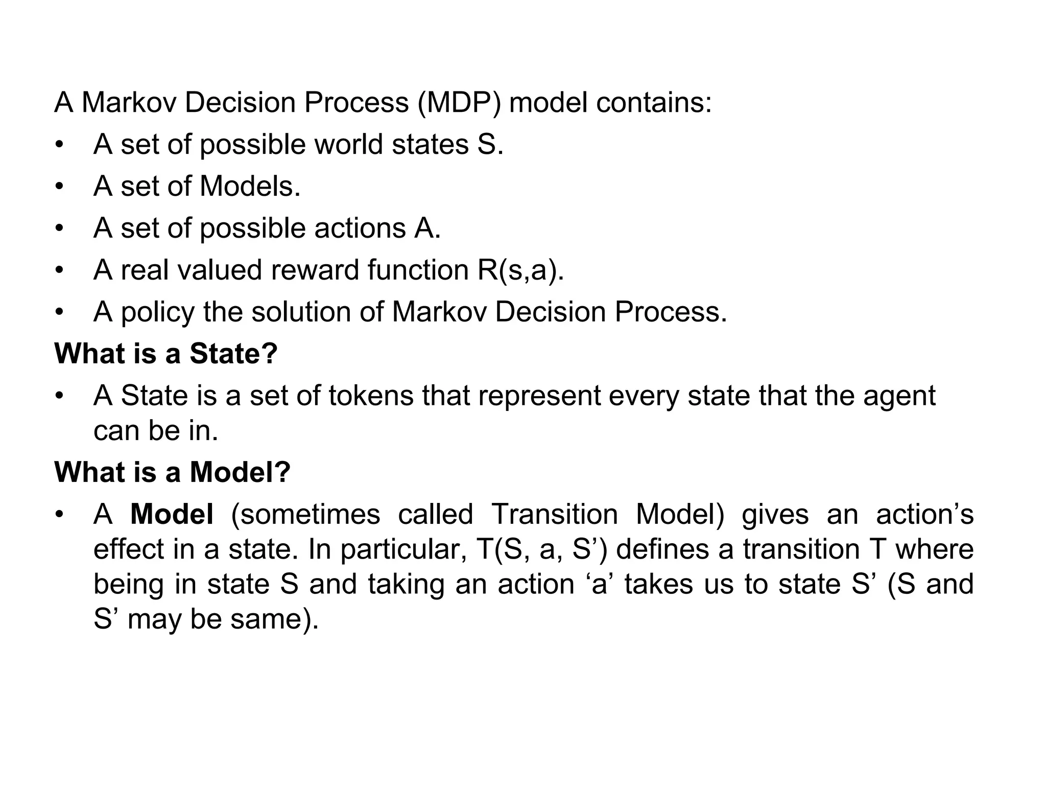
A Markov Decision Process (MDP) model contains:
• A set of possible world states S.
• A set of Models.
• A set of possible actions A.
• A real valued reward function R(s,a).
• A policy the solution of Markov Decision Process.
What is a State?
• A State is a set of tokens that represent every state that the agent
can be in.
What is a Model?
• A Model (sometimes called Transition Model) gives an action’s
effect in a state. In particular, T(S, a, S’) defines a transition T where
being in state S and taking an action ‘a’ takes us to state S’ (S and
S’ may be same).

• For stochastic actions (noisy, non-deterministic) we also define a
probability P(S’|S,a) which represents the probability of reaching a
state S’ if action ‘a’ is taken in state S. Note Markov property states
that the effects of an action taken in a state depend only on that
state and not on the prior history.
What is Actions?
• An Action A is set of all possible actions. A(s) defines the set of
actions that can be taken being in state S.
What is a Reward?
• A Reward is a real-valued reward function. R(s) indicates the
reward for simply being in the state S.
• R(S,a) indicates the reward for being in a state S and taking an
action ‘a’. R(S,a,S’) indicates the reward for being in a state S,
taking an action ‘a’ and ending up in a state S’.

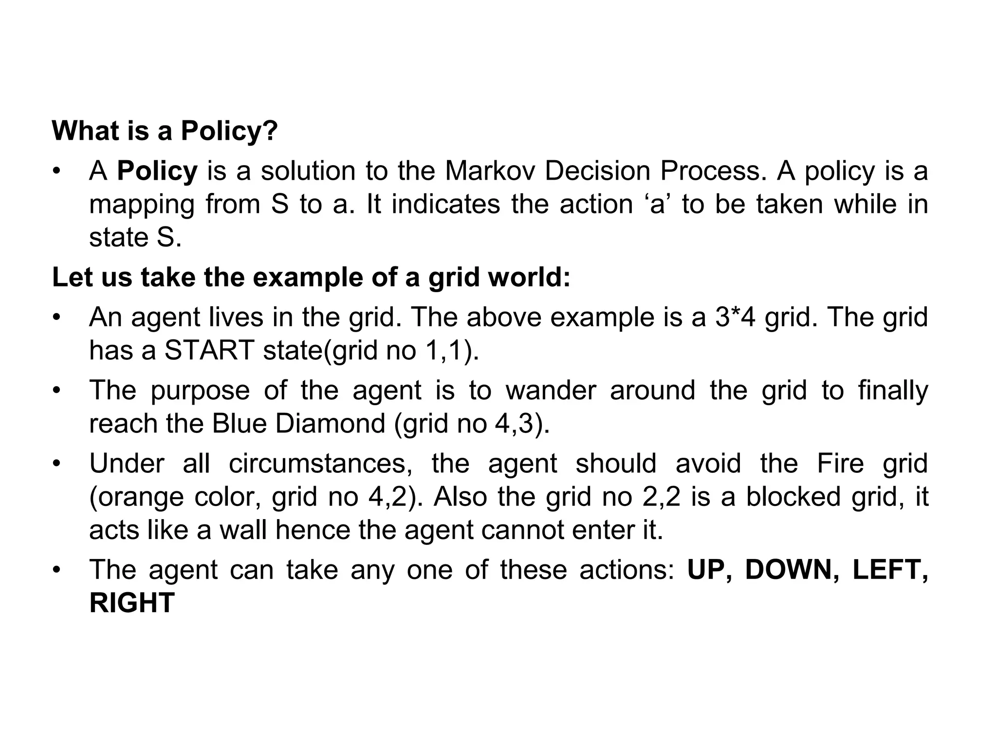
What is a Policy?
• A Policy is a solution to the Markov Decision Process. A policy is a
mapping from S to a. It indicates the action ‘a’ to be taken while in
state S.
Let us take the example of a grid world:
• An agent lives in the grid. The above example is a 3*4 grid. The grid
has a START state(grid no 1,1).
• The purpose of the agent is to wander around the grid to finally
reach the Blue Diamond (grid no 4,3).
• Under all circumstances, the agent should avoid the Fire grid
(orange color, grid no 4,2). Also the grid no 2,2 is a blocked grid, it
acts like a wall hence the agent cannot enter it.
• The agent can take any one of these actions: UP, DOWN, LEFT,
RIGHT

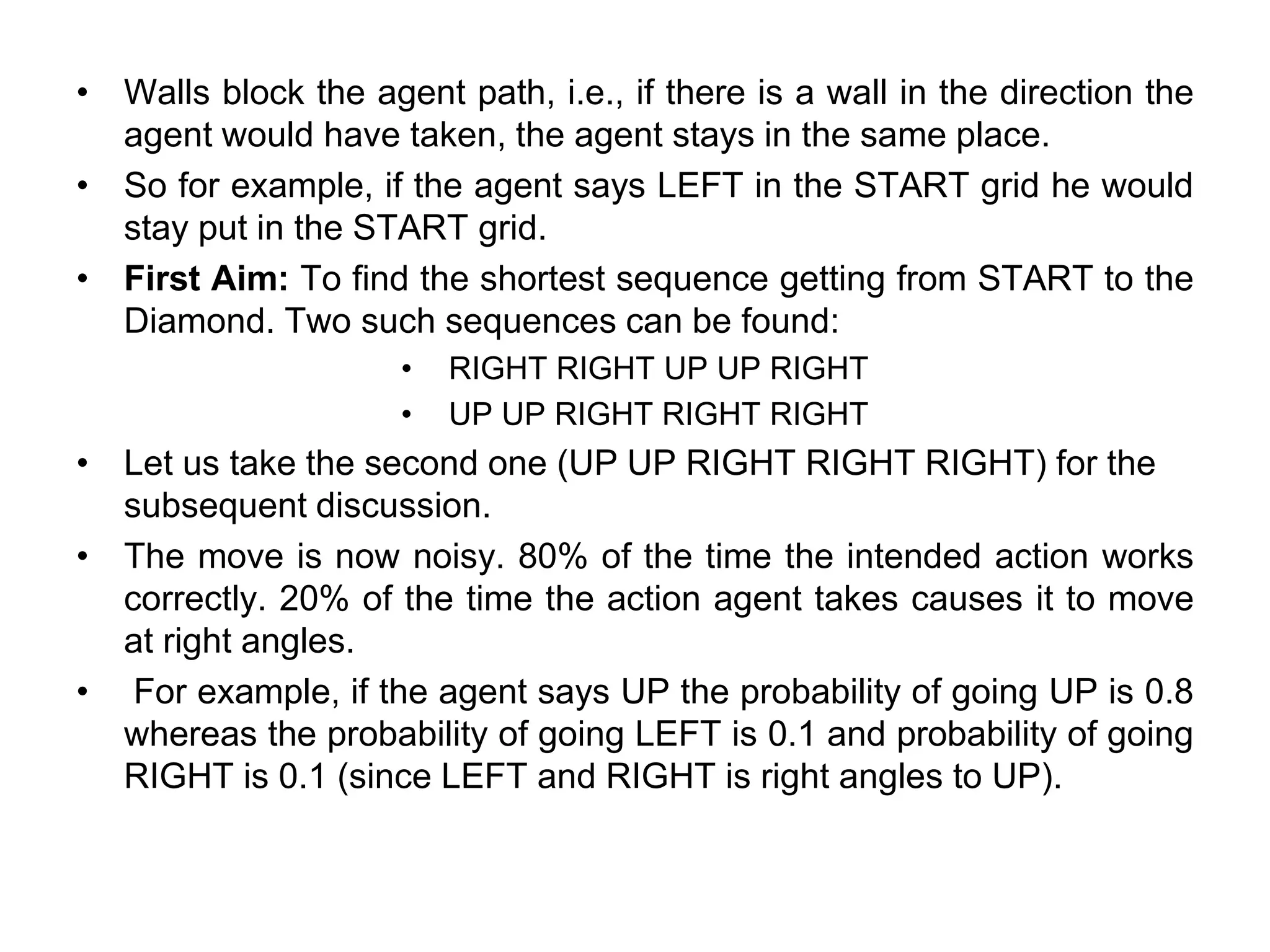
• Walls block the agent path, i.e., if there is a wall in the direction the
agent would have taken, the agent stays in the same place.
• So for example, if the agent says LEFT in the START grid he would
stay put in the START grid.
• First Aim: To find the shortest sequence getting from START to the
Diamond. Two such sequences can be found:
• RIGHT RIGHT UP UP RIGHT
• UP UP RIGHT RIGHT RIGHT
• Let us take the second one (UP UP RIGHT RIGHT RIGHT) for the
subsequent discussion.
• The move is now noisy. 80% of the time the intended action works
correctly. 20% of the time the action agent takes causes it to move
at right angles.
• For example, if the agent says UP the probability of going UP is 0.8
whereas the probability of going LEFT is 0.1 and probability of going
RIGHT is 0.1 (since LEFT and RIGHT is right angles to UP).

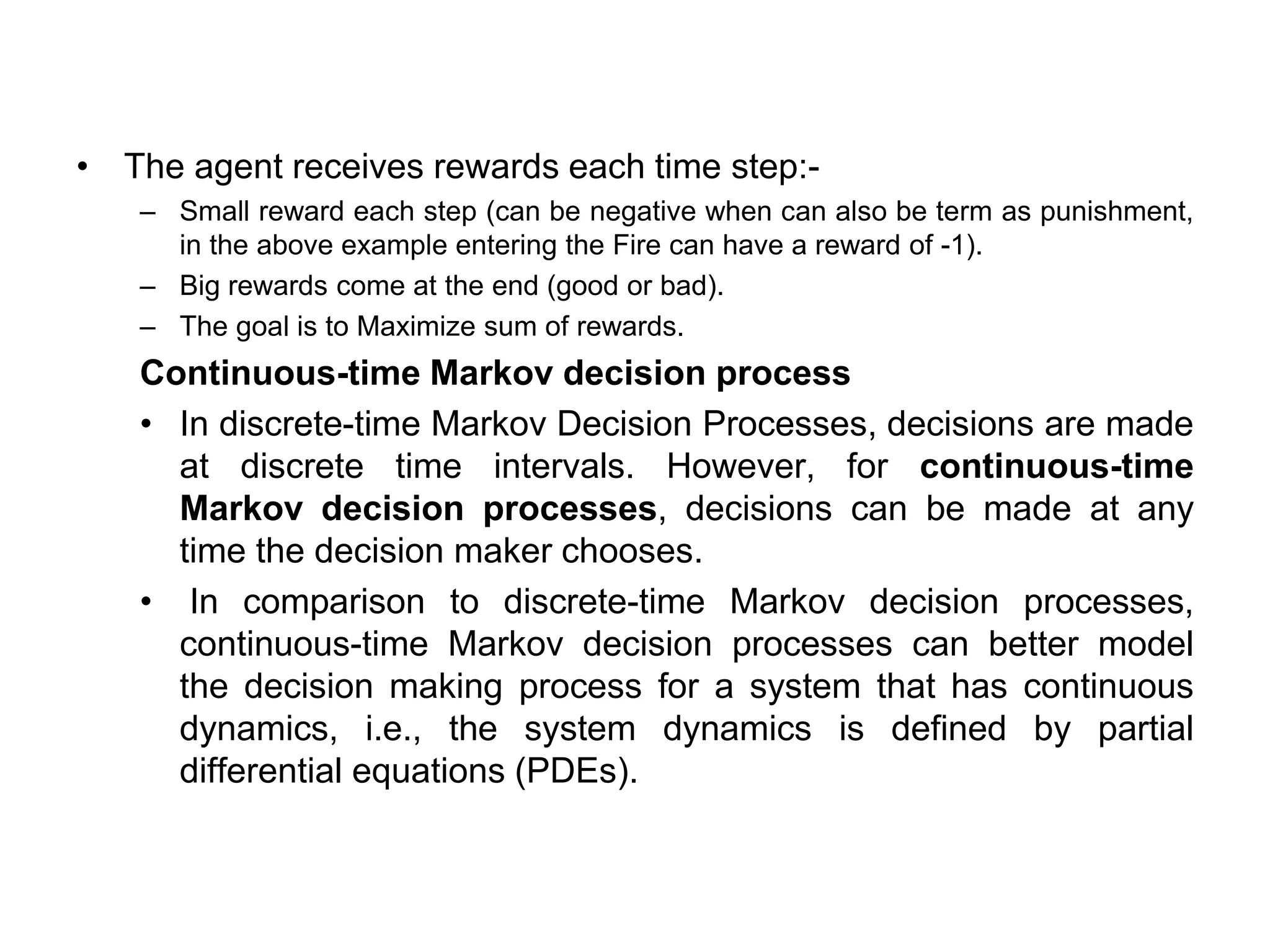
• The agent receives rewards each time step:-
– Small reward each step (can be negative when can also be term as punishment,
in the above example entering the Fire can have a reward of -1).
– Big rewards come at the end (good or bad).
– The goal is to Maximize sum of rewards.
Continuous-time Markov decision process
• In discrete-time Markov Decision Processes, decisions are made
at discrete time intervals. However, for continuous-time
Markov decision processes, decisions can be made at any
time the decision maker chooses.
• In comparison to discrete-time Markov decision processes,
continuous-time Markov decision processes can better model
the decision making process for a system that has continuous
dynamics, i.e., the system dynamics is defined by partial
differential equations (PDEs).

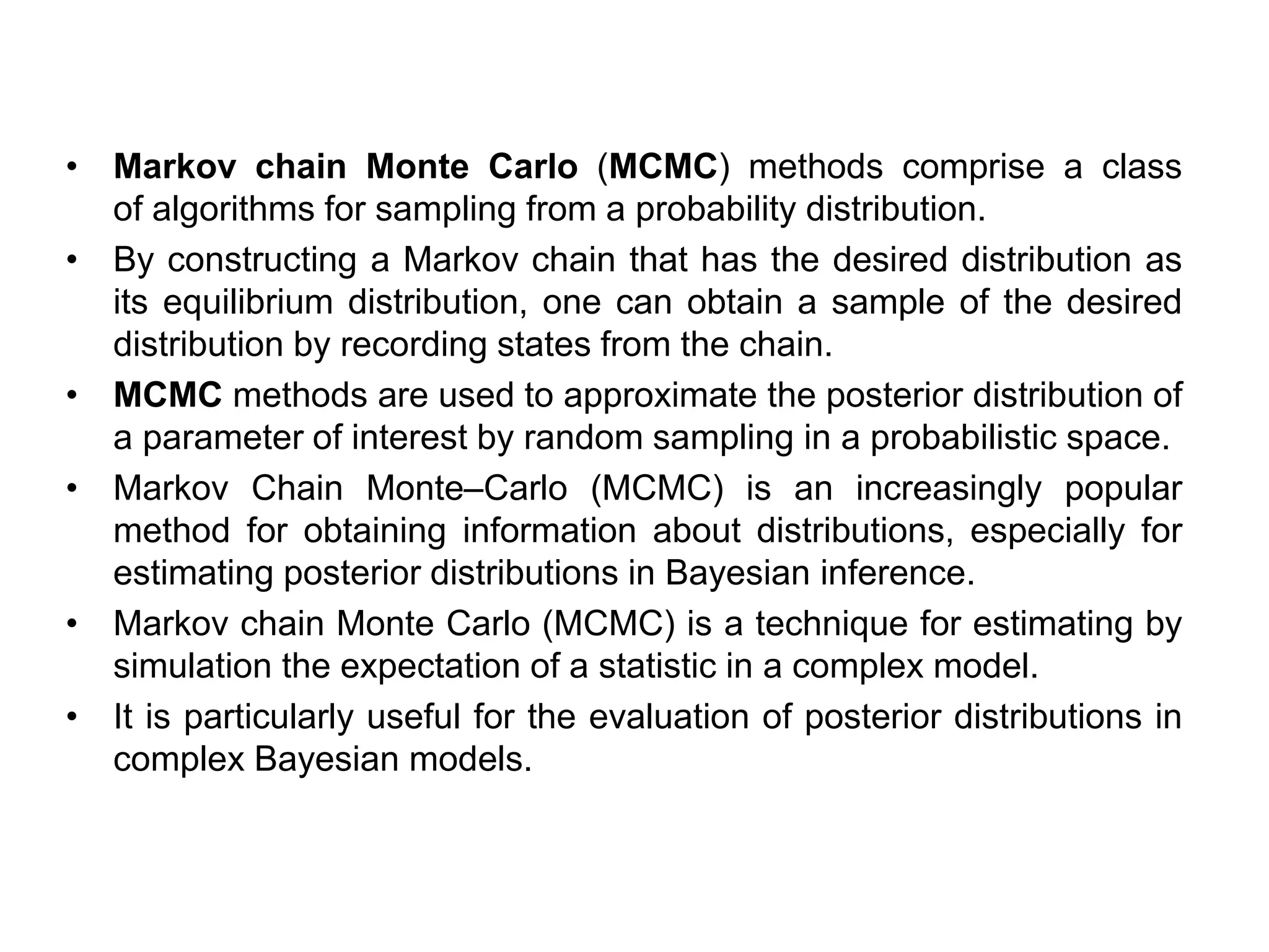
• Markov chain Monte Carlo (MCMC) methods comprise a class
of algorithms for sampling from a probability distribution.
• By constructing a Markov chain that has the desired distribution as
its equilibrium distribution, one can obtain a sample of the desired
distribution by recording states from the chain.
• MCMC methods are used to approximate the posterior distribution of
a parameter of interest by random sampling in a probabilistic space.
• Markov Chain Monte–Carlo (MCMC) is an increasingly popular
method for obtaining information about distributions, especially for
estimating posterior distributions in Bayesian inference.
• Markov chain Monte Carlo (MCMC) is a technique for estimating by
simulation the expectation of a statistic in a complex model.
• It is particularly useful for the evaluation of posterior distributions in
complex Bayesian models.

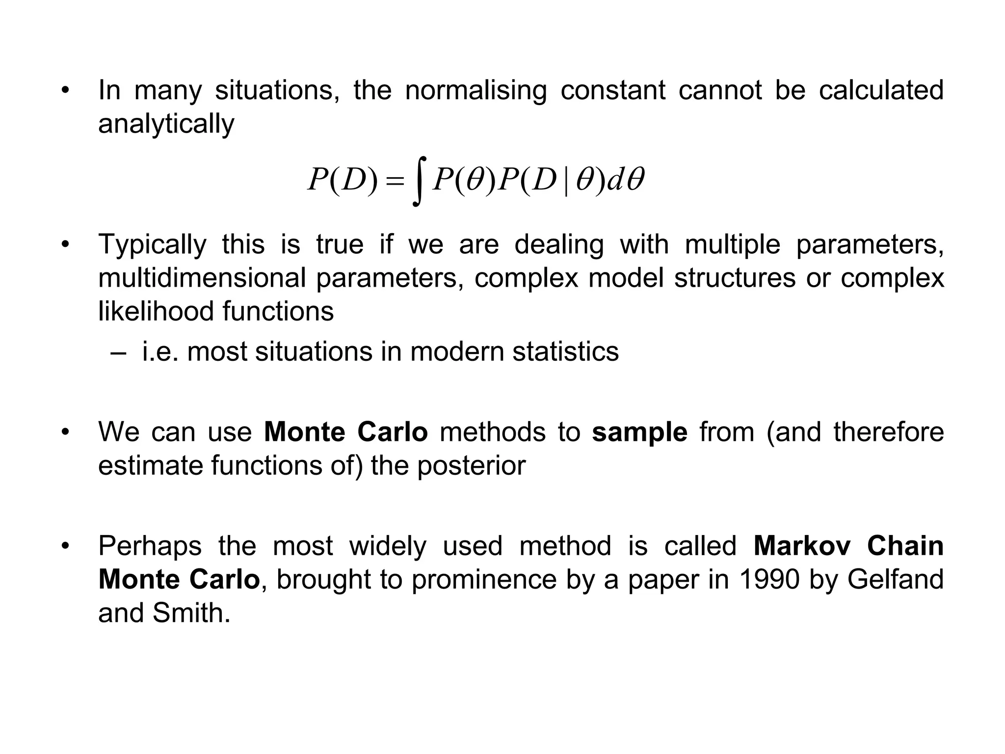
• In many situations, the normalising constant cannot be calculated
analytically
• Typically this is true if we are dealing with multiple parameters,
multidimensional parameters, complex model structures or complex
likelihood functions
– i.e. most situations in modern statistics
• We can use Monte Carlo methods to sample from (and therefore
estimate functions of) the posterior
• Perhaps the most widely used method is called Markov Chain
Monte Carlo, brought to prominence by a paper in 1990 by Gelfand
and Smith.
=  dDPPDP )|()()(

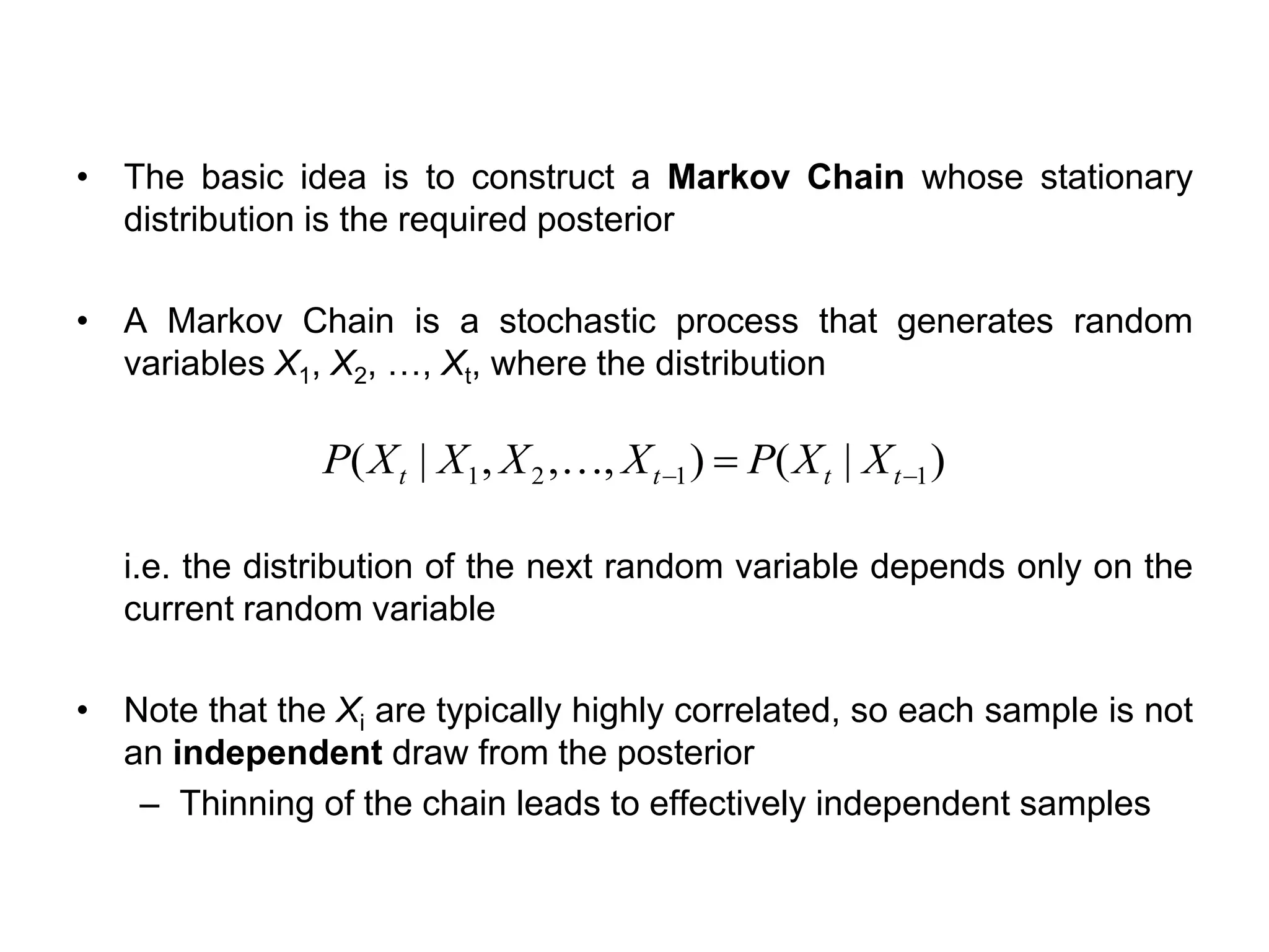
• The basic idea is to construct a Markov Chain whose stationary
distribution is the required posterior
• A Markov Chain is a stochastic process that generates random
variables X1, X2, …, Xt, where the distribution
i.e. the distribution of the next random variable depends only on the
current random variable
• Note that the Xi are typically highly correlated, so each sample is not
an independent draw from the posterior
– Thinning of the chain leads to effectively independent samples
)|(),,,|( 1121 −− = tttt XXPXXXXP 

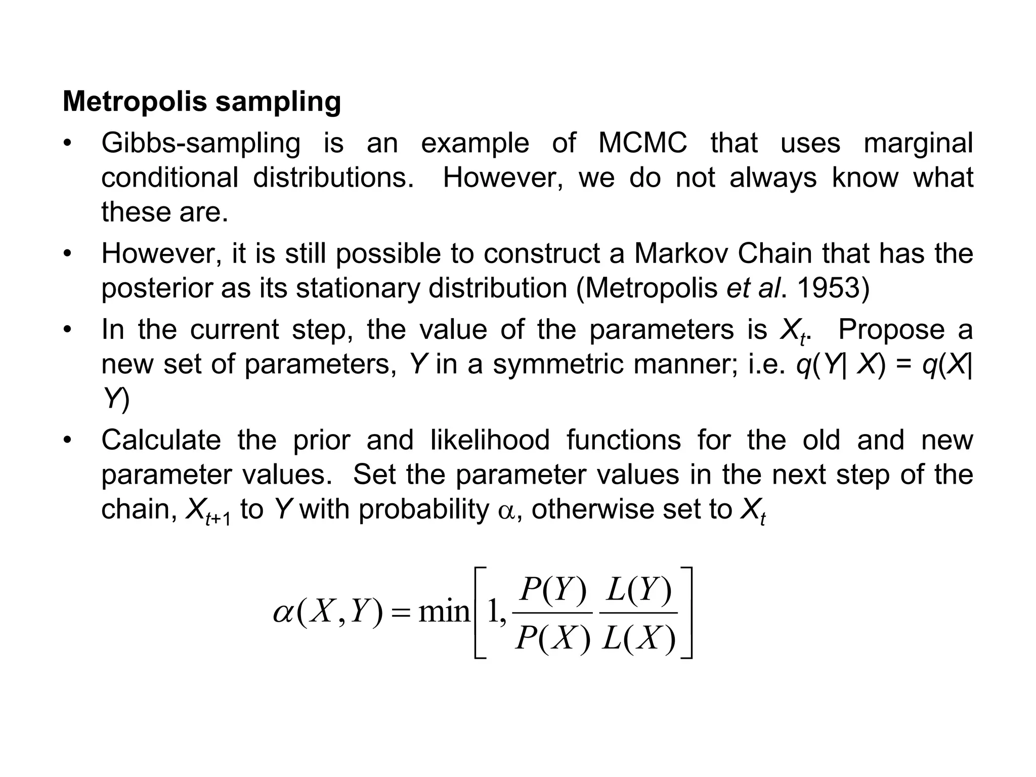
Metropolis sampling
• Gibbs-sampling is an example of MCMC that uses marginal
conditional distributions. However, we do not always know what
these are.
• However, it is still possible to construct a Markov Chain that has the
posterior as its stationary distribution (Metropolis et al. 1953)
• In the current step, the value of the parameters is Xt. Propose a
new set of parameters, Y in a symmetric manner; i.e. q(Y| X) = q(X|
Y)
• Calculate the prior and likelihood functions for the old and new
parameter values. Set the parameter values in the next step of the
chain, Xt+1 to Y with probability a, otherwise set to Xt






=
)(
)(
)(
)(
,1min),(
XL
YL
XP
YP
YXa

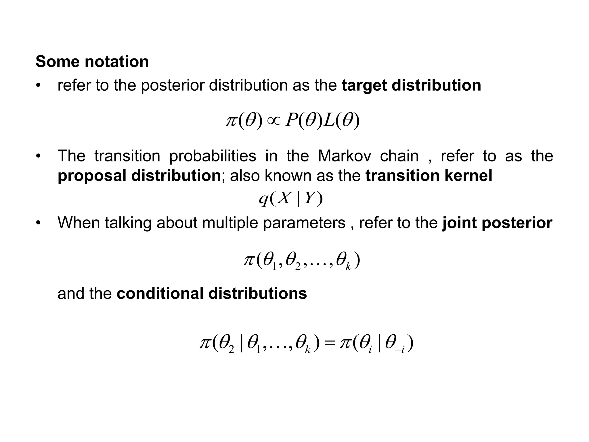
Some notation
• refer to the posterior distribution as the target distribution
• The transition probabilities in the Markov chain , refer to as the
proposal distribution; also known as the transition kernel
• When talking about multiple parameters , refer to the joint posterior
and the conditional distributions
)()()(  LP
)|( YXq
),,,( 21 k 
)|(),,|( 12 iik −=  

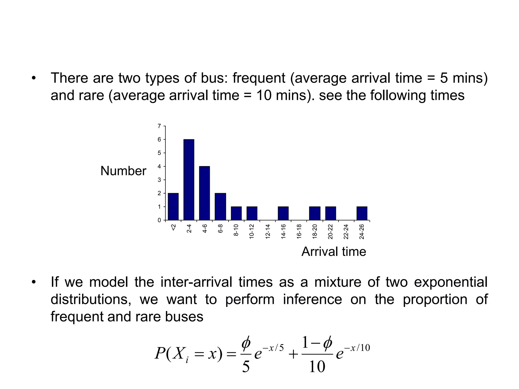
• There are two types of bus: frequent (average arrival time = 5 mins)
and rare (average arrival time = 10 mins). see the following times
• If we model the inter-arrival times as a mixture of two exponential
distributions, we want to perform inference on the proportion of
frequent and rare buses
0
1
2
3
4
5
6
7
<2
2-4
4-6
6-8
8-10
10-12
12-14
14-16
16-18
18-20
20-22
22-24
24-26
Arrival time
Number
10/5/
10
1
5
)( xx
i eexXP −− −
+==


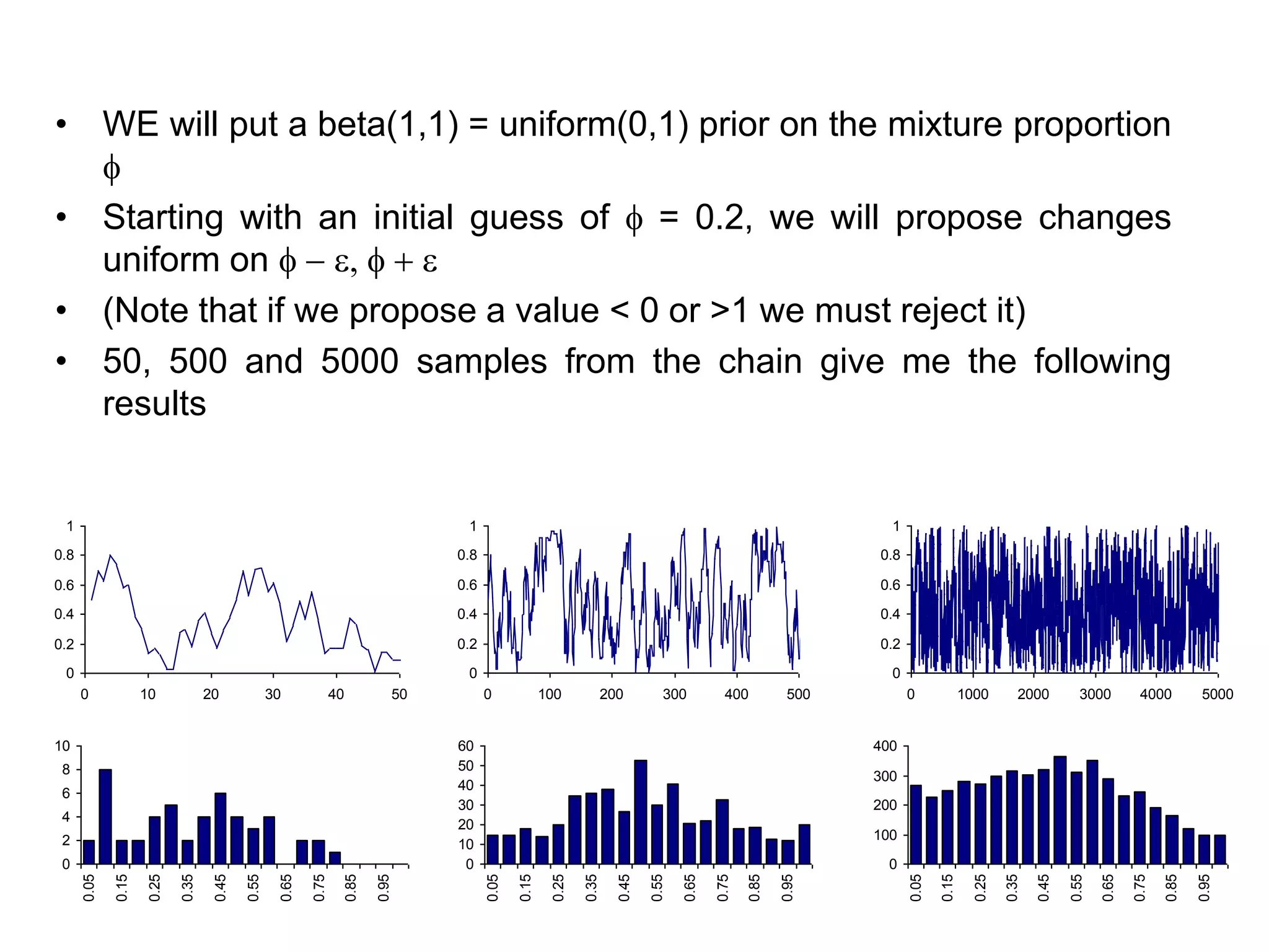
• WE will put a beta(1,1) = uniform(0,1) prior on the mixture proportion

• Starting with an initial guess of  = 0.2, we will propose changes
uniform on  − e,  + e
• (Note that if we propose a value < 0 or >1 we must reject it)
• 50, 500 and 5000 samples from the chain give me the following
results
0
0.2
0.4
0.6
0.8
1
0 10 20 30 40 50
0
0.2
0.4
0.6
0.8
1
0 100 200 300 400 500
0
0.2
0.4
0.6
0.8
1
0 1000 2000 3000 4000 5000
0
2
4
6
8
10
0.05
0.15
0.25
0.35
0.45
0.55
0.65
0.75
0.85
0.95
0
10
20
30
40
50
60
0.05
0.15
0.25
0.35
0.45
0.55
0.65
0.75
0.85
0.95
0
100
200
300
400
0.05
0.15
0.25
0.35
0.45
0.55
0.65
0.75
0.85
0.95

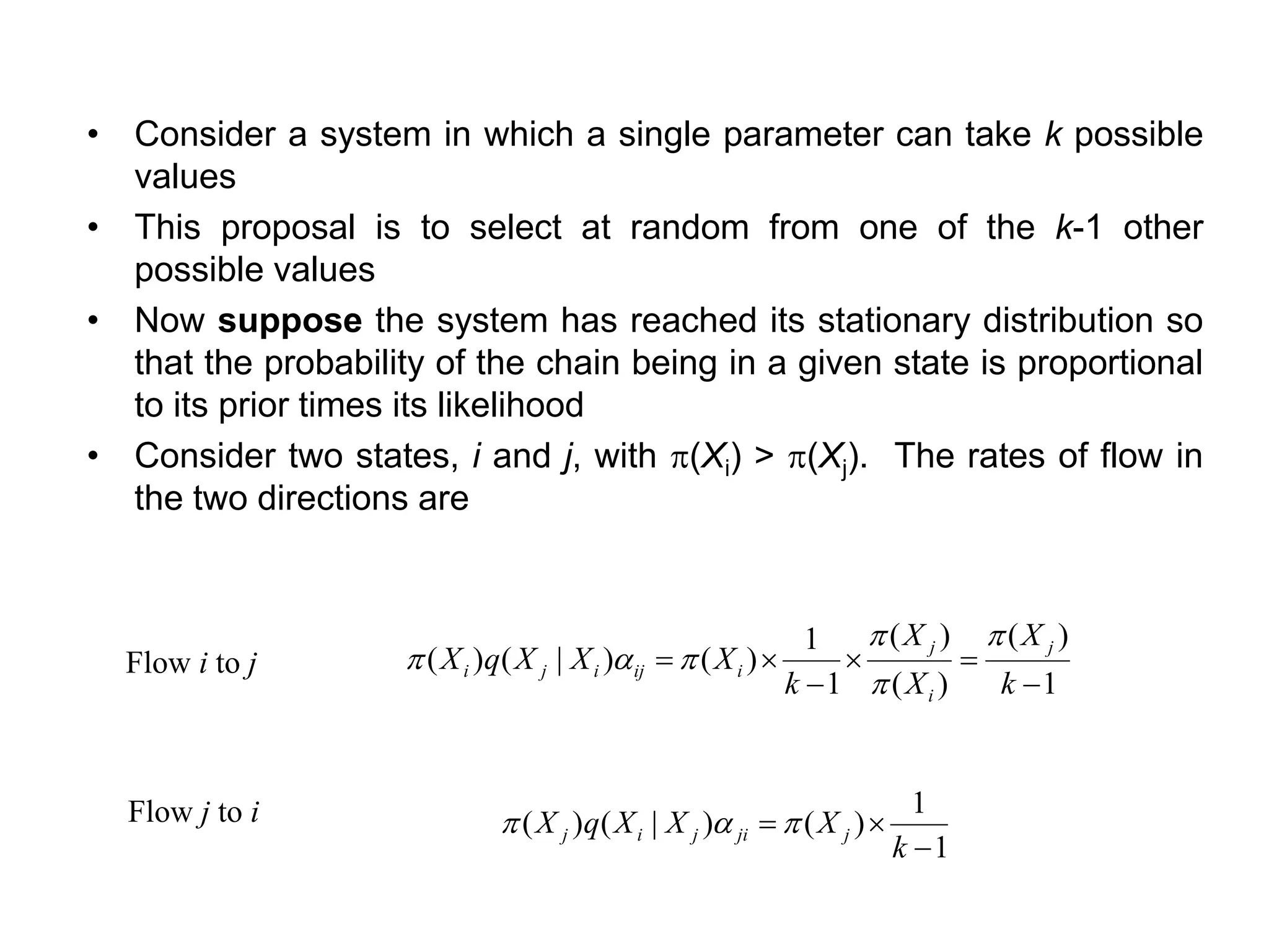
• Consider a system in which a single parameter can take k possible
values
• This proposal is to select at random from one of the k-1 other
possible values
• Now suppose the system has reached its stationary distribution so
that the probability of the chain being in a given state is proportional
to its prior times its likelihood
• Consider two states, i and j, with (Xi) > (Xj). The rates of flow in
the two directions are
1
)(
)(
)(
1
1
)()|()(
−
=
−
=
k
X
X
X
k
XXXqX
j
i
j
iijiji



a
1
1
)()|()(
−
=
k
XXXqX jjijij a
Flow i to j
Flow j to i

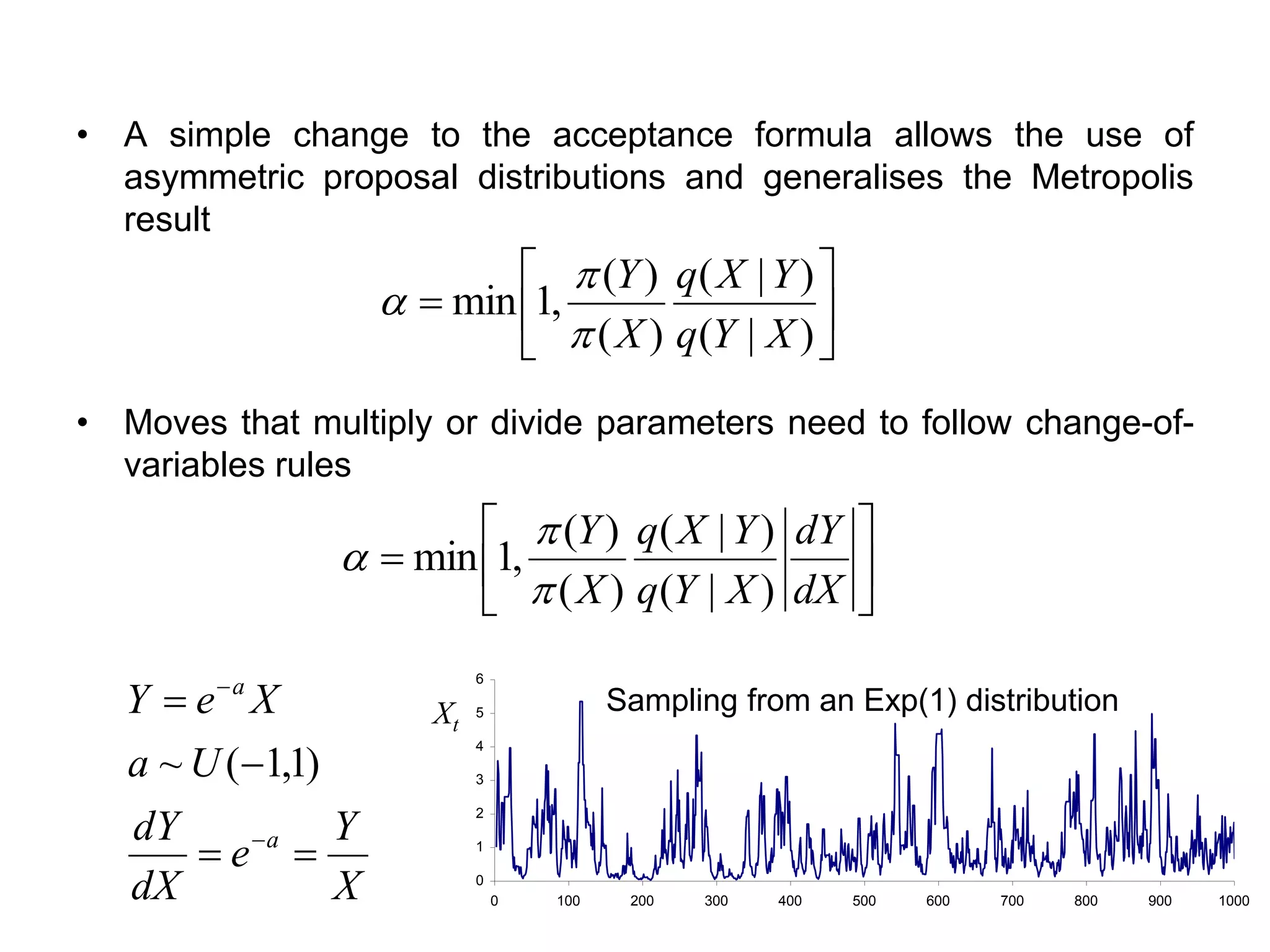
• A simple change to the acceptance formula allows the use of
asymmetric proposal distributions and generalises the Metropolis
result
• Moves that multiply or divide parameters need to follow change-of-
variables rules






=
)|(
)|(
)(
)(
,1min
XYq
YXq
X
Y


a






=
dX
dY
XYq
YXq
X
Y
)|(
)|(
)(
)(
,1min


a
X
Y
e
dX
dY
Ua
XeY
a
a
==
−
=
−
−
)1,1(~
0
1
2
3
4
5
6
0 100 200 300 400 500 600 700 800 900 1000
Sampling from an Exp(1) distributionXt

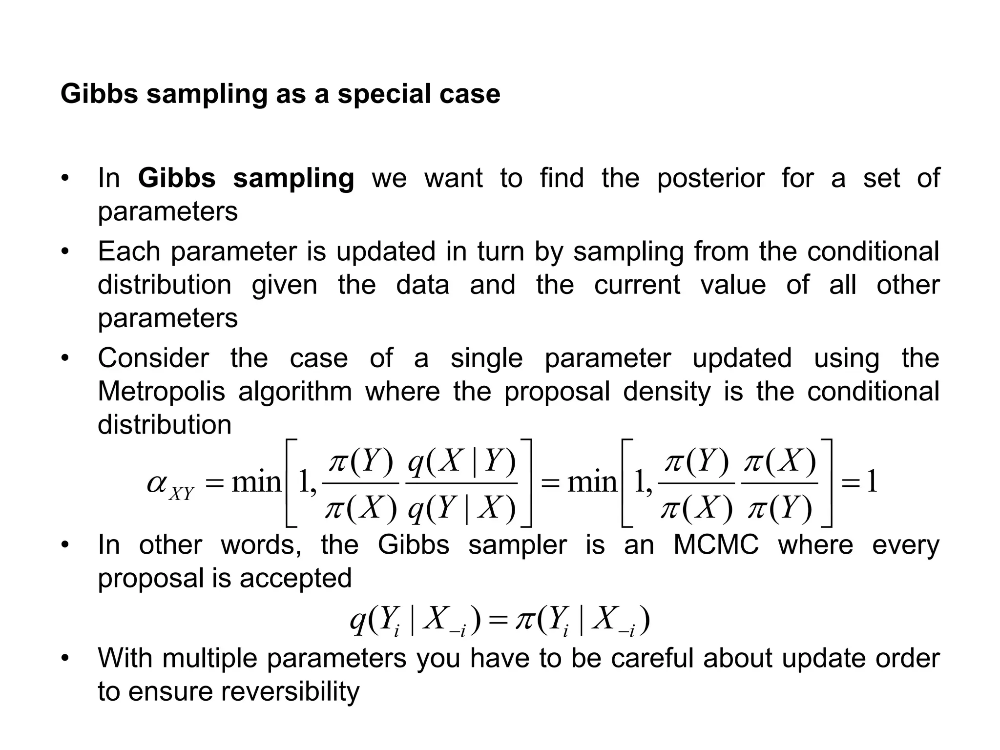
Gibbs sampling as a special case
• In Gibbs sampling we want to find the posterior for a set of
parameters
• Each parameter is updated in turn by sampling from the conditional
distribution given the data and the current value of all other
parameters
• Consider the case of a single parameter updated using the
Metropolis algorithm where the proposal density is the conditional
distribution
• In other words, the Gibbs sampler is an MCMC where every
proposal is accepted
• With multiple parameters you have to be careful about update order
to ensure reversibility
1
)(
)(
)(
)(
,1min
)|(
)|(
)(
)(
,1min =





=





=
Y
X
X
Y
XYq
YXq
X
Y
XY






a
)|()|( iiii XYXYq −− =

Convergence
• The Markov Chain is guaranteed to have the posterior as its
stationary distribution (if well constructed)
• BUT this does not tell you how long you have to run the chain in
order to reach stationarity
– The initial starting point may have a strong influence
– The proposal distributions may lead to low acceptance rates
– The likelihood surface may have local maxima that trap the chain
• Multiple runs from different initial conditions and graphical checks
can be used to assess convergence
– The efficiency of a chain can be measured in terms of the
variance of estimates obtained by running the chain for a short
period of time

Watching the chain 2
0
1
2
3
4
5
6
7
0 100 200 300 400 500 600 700 800 900 1000
20
0
1
2
3
4
5
6
7
0 100 200 300 400 500 600 700 800 900 1000
200
0
1
2
3
4
5
6
7
0 100 200 300 400 500 600 700 800 900 1000
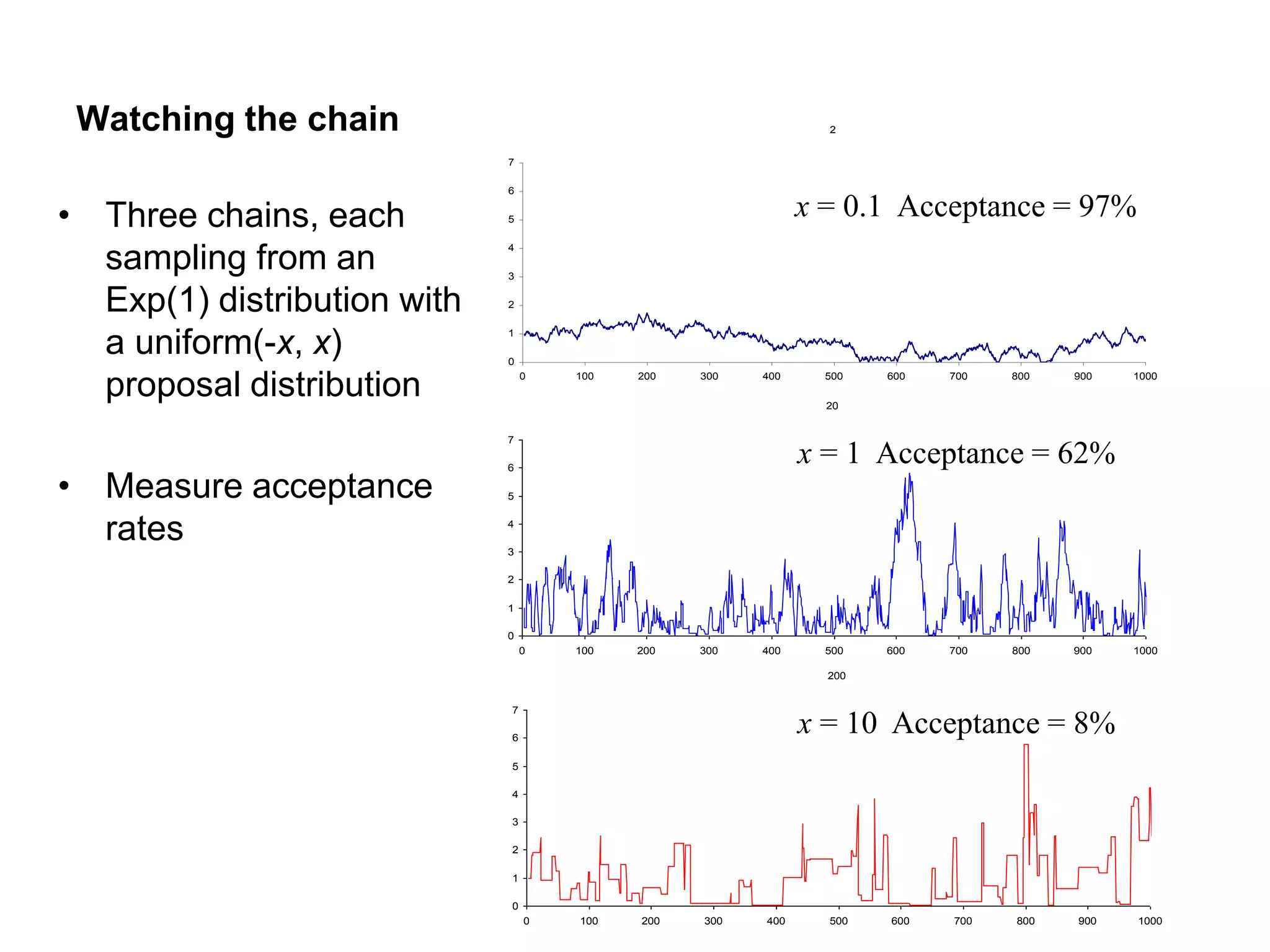
• Three chains, each
sampling from an
Exp(1) distribution with
a uniform(-x, x)
proposal distribution
• Measure acceptance
rates
x = 0.1 Acceptance = 97%
x = 1 Acceptance = 62%
x = 10 Acceptance = 8%

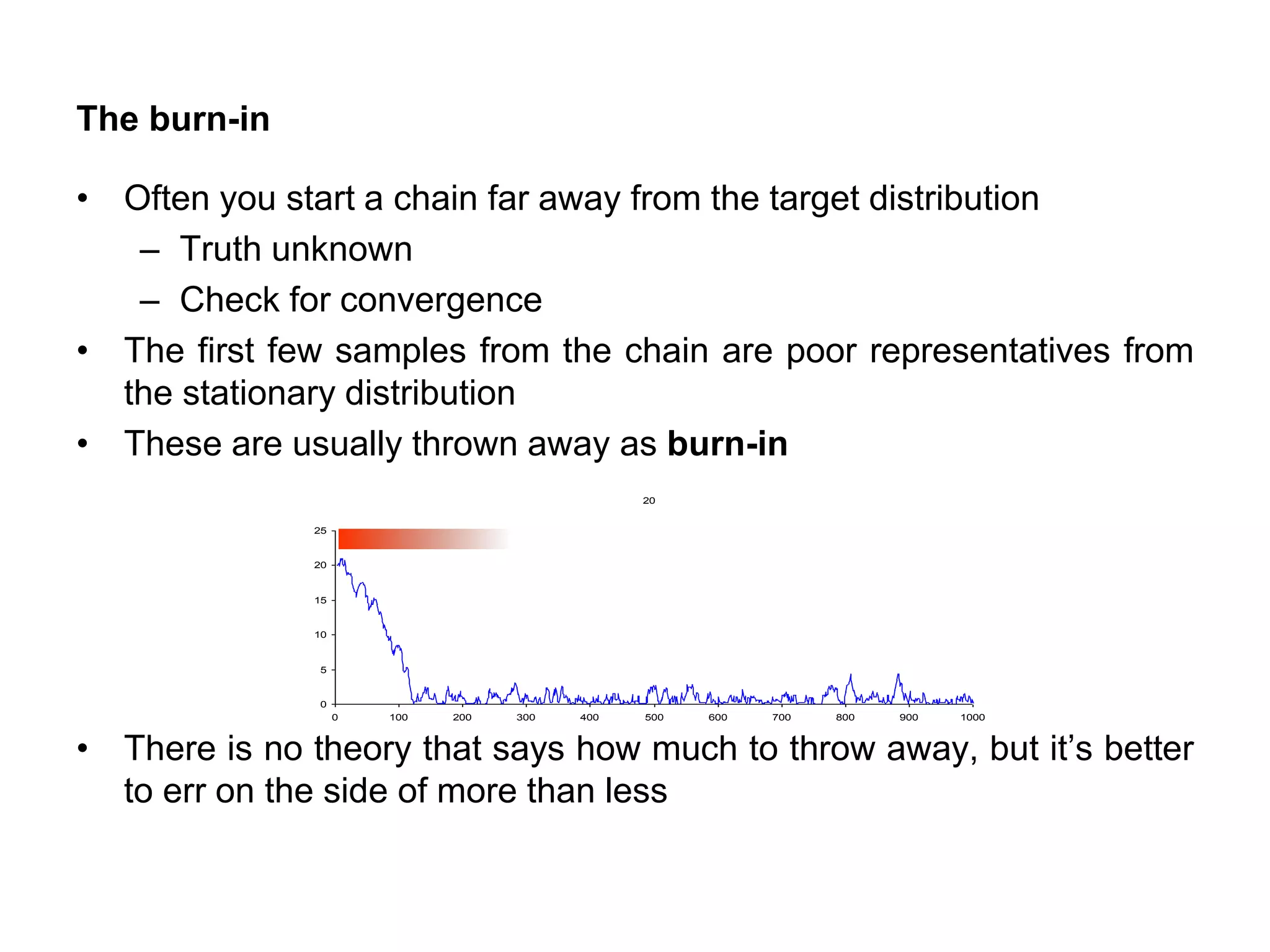
The burn-in
• Often you start a chain far away from the target distribution
– Truth unknown
– Check for convergence
• The first few samples from the chain are poor representatives from
the stationary distribution
• These are usually thrown away as burn-in
• There is no theory that says how much to throw away, but it’s better
to err on the side of more than less
20
0
5
10
15
20
25
0 100 200 300 400 500 600 700 800 900 1000

Other uses of MCMC
• Looking at marginal effects
– Suppose we have a multidimensional parameter, we may just
want to know about the marginal posterior distribution of that
parameter
• Prediction
– Given our posterior distribution on parameters, we can predict
the distribution of future data by sampling parameters from the
posterior and simulating data given those parameters
– The posterior predictive distribution is a useful source of
goodness-of-fit testing (if predicted data doesn’t look like the
data you’ve collected, the model is poor)

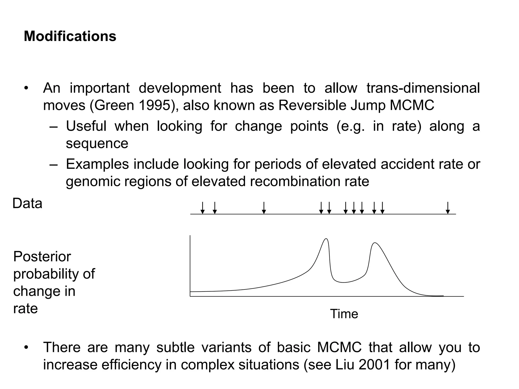
Modifications
• An important development has been to allow trans-dimensional
moves (Green 1995), also known as Reversible Jump MCMC
– Useful when looking for change points (e.g. in rate) along a
sequence
– Examples include looking for periods of elevated accident rate or
genomic regions of elevated recombination rate
• There are many subtle variants of basic MCMC that allow you to
increase efficiency in complex situations (see Liu 2001 for many)
Posterior
probability of
change in
rate
Data
Time

More advanced sampling techniques
• Auxiliary variable samplers
– Hybrid Monte Carlo
• Uses the gradient of p
– Tries to avoid ‘random walk’ behavior, i.e. to speed up
convergence
• Reversible jump MCMC
– For comparing models of different dimensionalities (in ‘model
selection’ problems)
• Adaptive MCMC
– Trying to automate the choice of q

• Two main families of approximate algorithms: variational methods
(Variational inference methods take their name from the calculus of
variations, which deals with optimizing functions that take other
functions as arguments) which formulate inference as an
optimization problem, as well as sampling methods, which produce
answers by repeatedly generating random numbers from a
distribution of interest.
• Sampling provides a flexible way to approximate many sums and
integrals at reduced cost.
• Sampling methods can be used to perform both marginal and MAP
inference queries; in addition, they can compute various interesting
quantities, such as expectations E[f(X)] of random variables
distributed according to a given probabilistic model.

Sampling from a probability distribution
As a warm-up, let’s think for a minute how we might sample
from a multinomial distribution with kk possible outcomes and
associated probabilities θ1,…,θk.
Sampling, in general, is not an easy problem. Our computers
can only generate samples from very simple such as the uniform
distribution over [0,1]. All sampling techniques involve calling some kind
of simple subroutine multiple times in a clever way.
In our case, we may reduce sampling from a multinomial
variable to sampling a single uniform variable by subdividing a unit
interval into k regions with region i having size θi. We then sample
uniformly from [0,1] and return the value of the region in which our
sample falls.
Reducing sampling from a multinomial
distribution to sampling a uniform distribution in
[0,1].

Forward Sampling
• “Forward sampling” can also be performed efficiently on undirected
models if the model can be represented by a clique tree with a small
number of variables per node.
• Calibrate the clique tree, which gives us the marginal distribution
over each node, and choose a node to be the root. Then,
marginalize over variables in the root node to get the marginal for a
single variable.
• Once the marginal for a single variable x1∼p(X1∣E=e) has been
sampled from the root node, the newly sampled value X1=x1can be
incorporated as evidence.
• Finish sampling other variables from the same node, each time
incorporating the newly sampled nodes as evidence,
i.e. x2∼p(X2=x2∣X1=x1,E=e)
and x3∼p(X3=x3∣X1=x1,X2=x2,E=e) and so on.
• When moving down the tree to sample variables from other nodes,
each node must send an updated message containing the values of
the sampled variables.

Rejection sampling
• A special case of Monte Carlo integration is rejection sampling. We
may use it to compute the area of a region R by sampling in a larger
region with a known area and recording the fraction of samples that
falls within R.
Importance sampling
• Unfortunately, rejection sampling can be very wasteful.
If p(E=e) equals, say, 1%, then we will discard 99% of all samples.
• A better way of computing such integrals uses importance sampling.
The main idea is to sample from a distribution q (hopefully
with q(x) roughly proportional to f(x)⋅p(x), and then reweigh the
samples in a principled way, so that their sum still approximates the
desired integral.

CSA 3702 machine learning module 4

In this document

More Related Content

What's hot

Similar to CSA 3702 machine learning module 4

Recently uploaded

CSA 3702 machine learning module 4