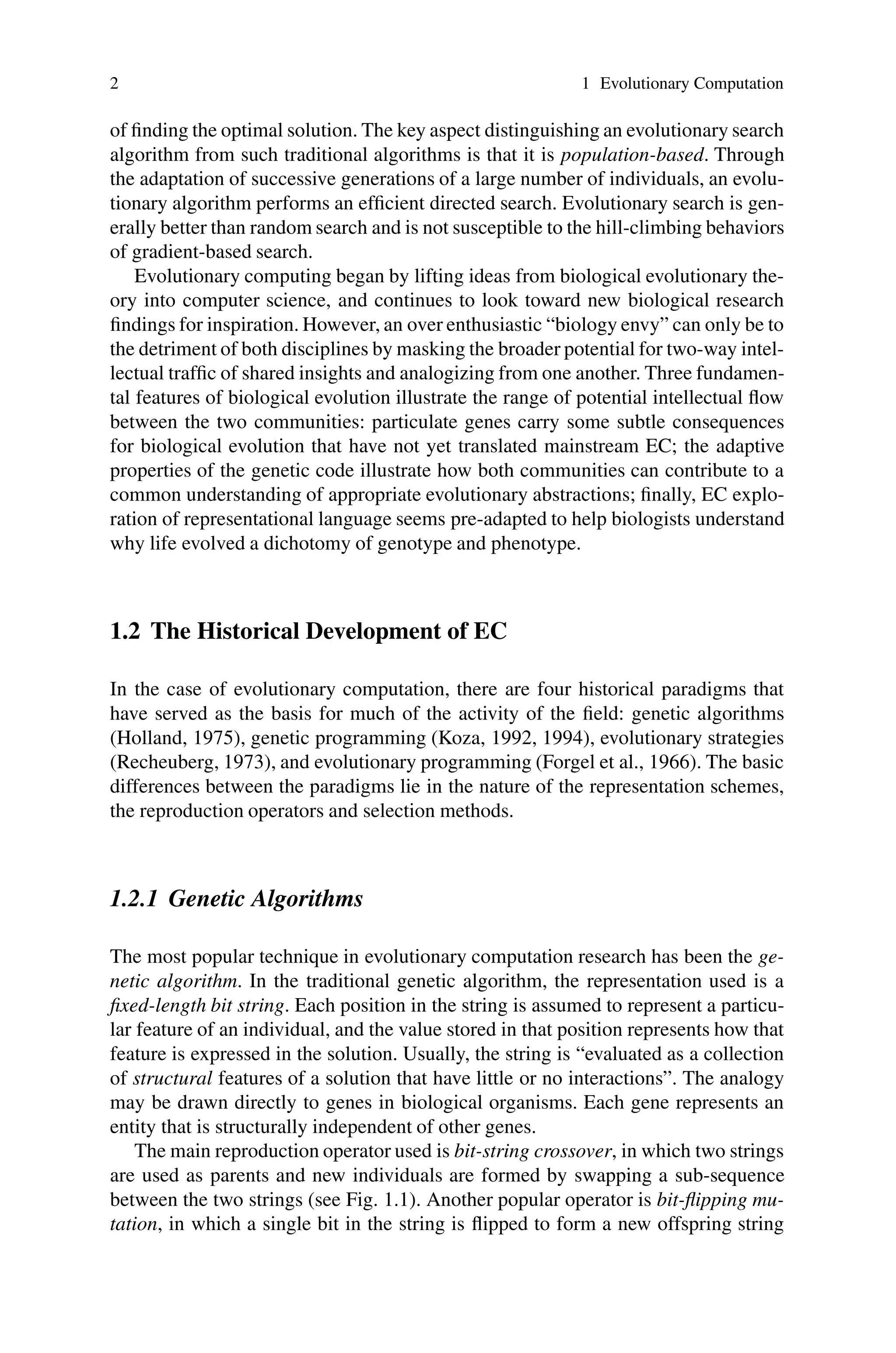
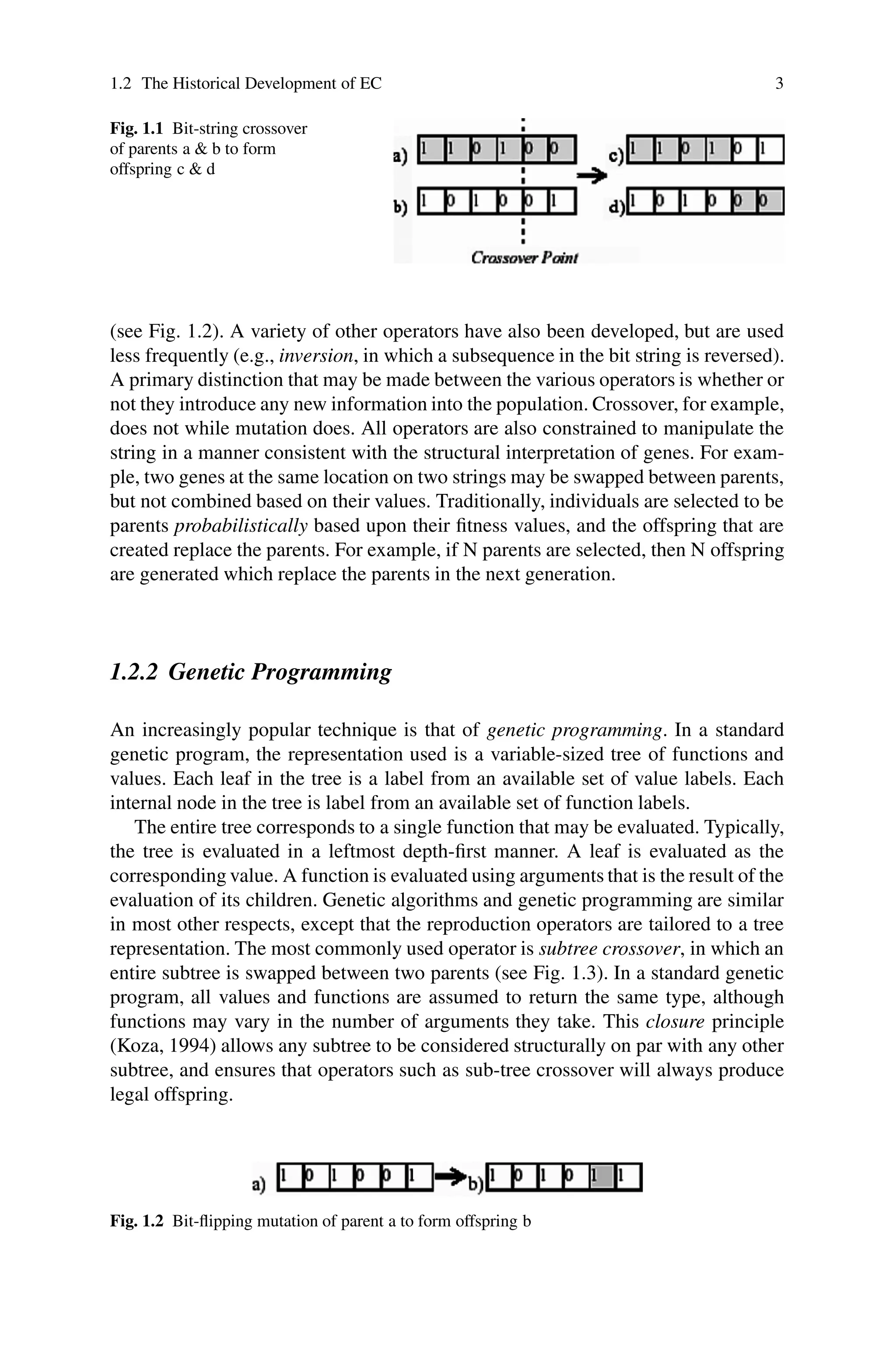
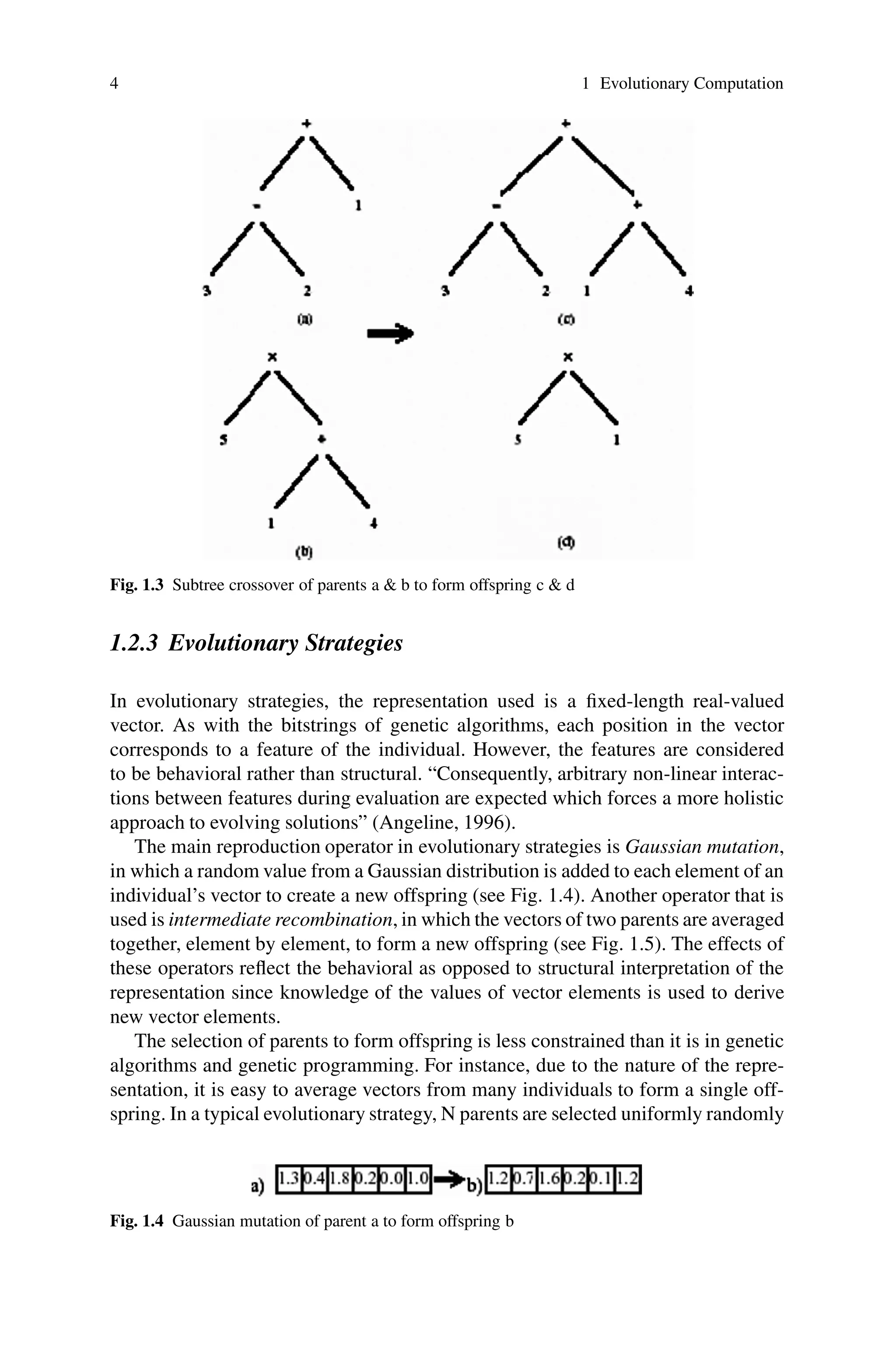
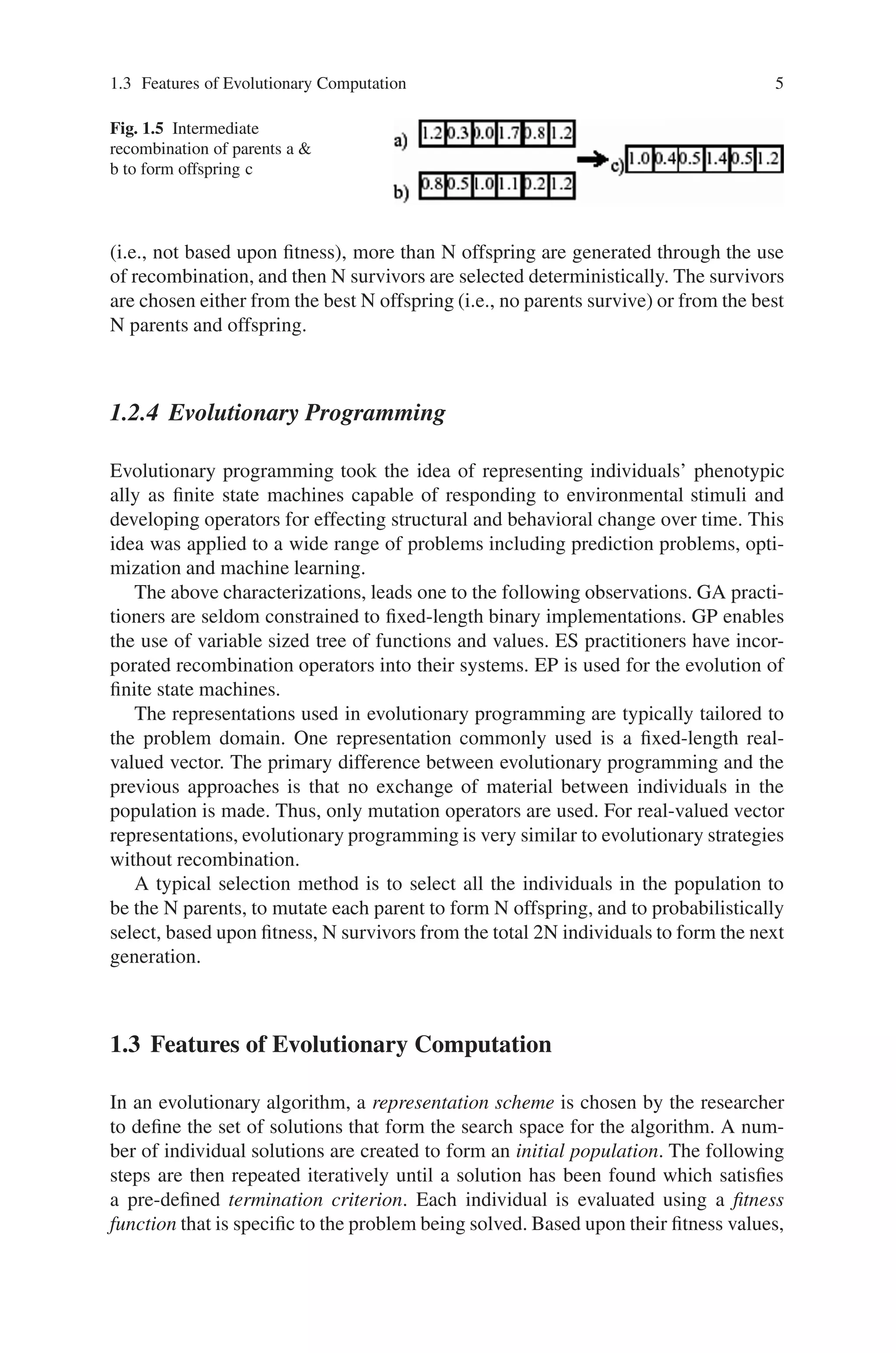
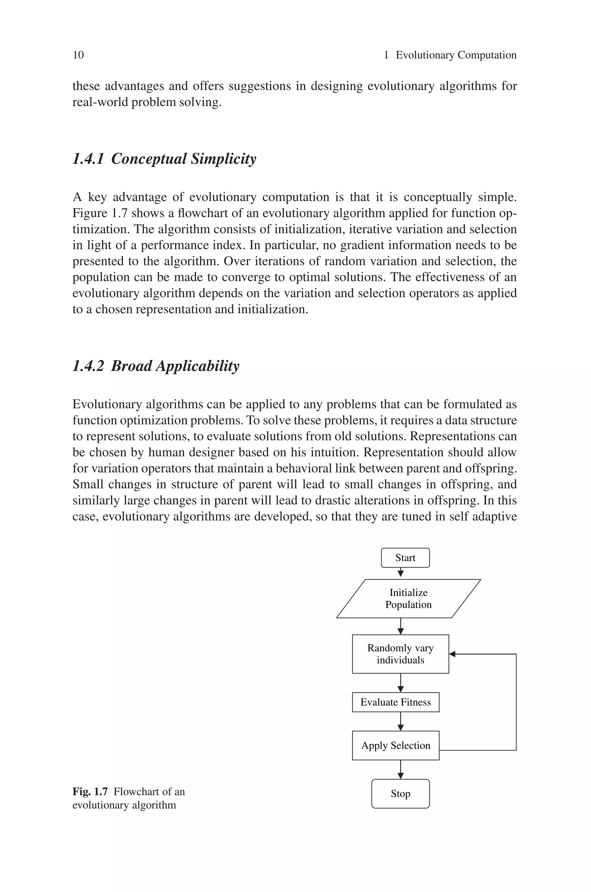
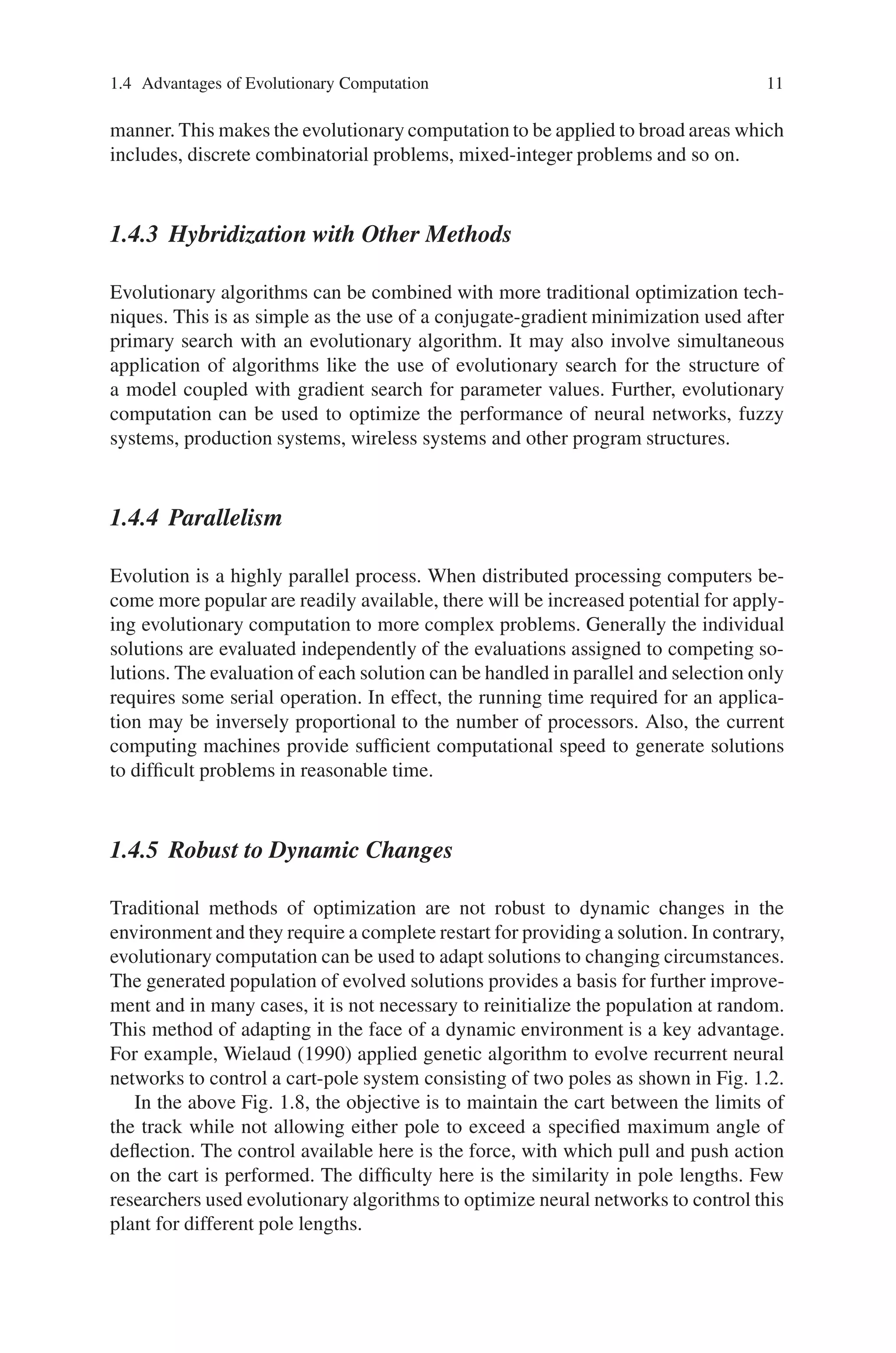
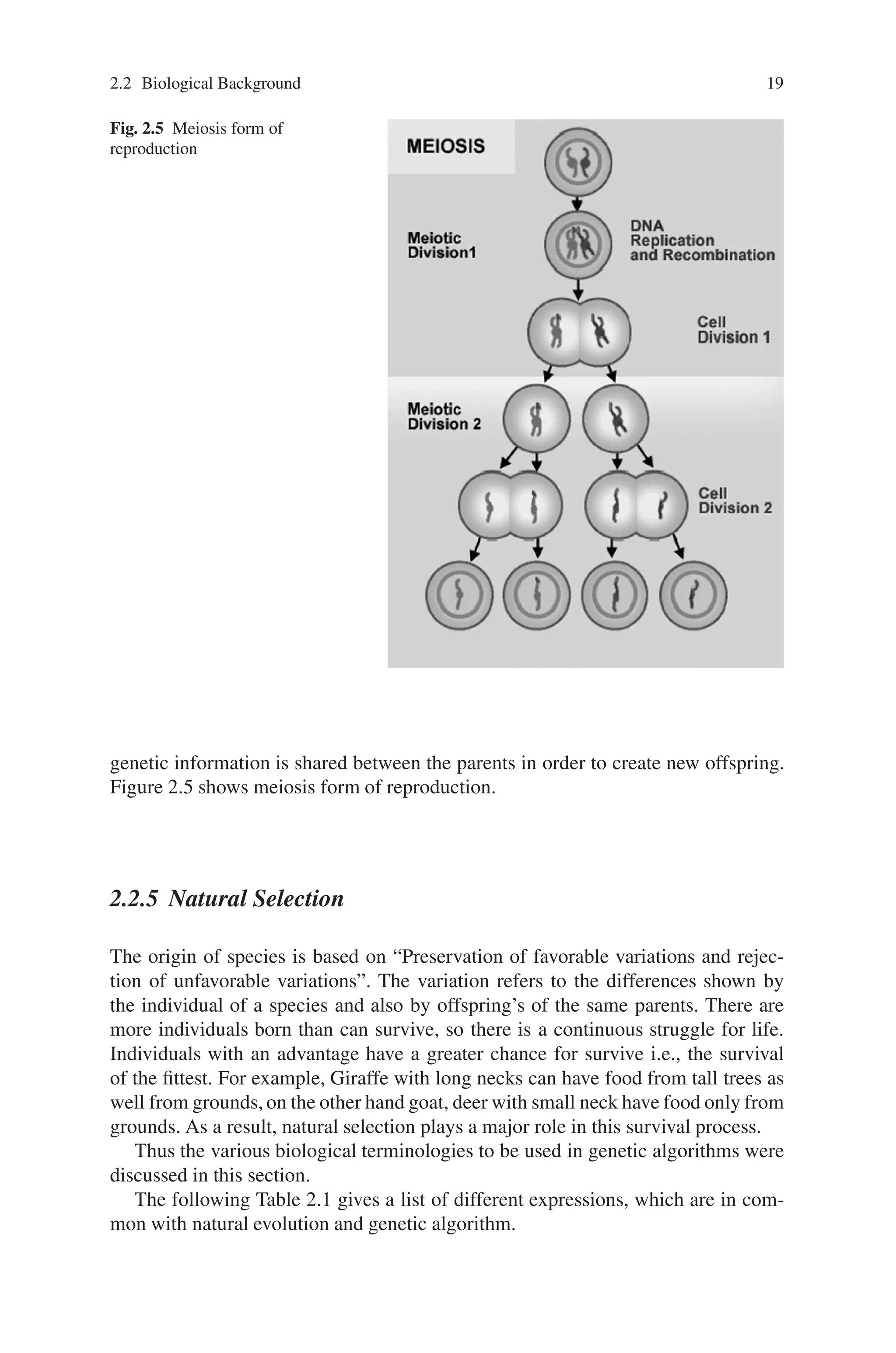
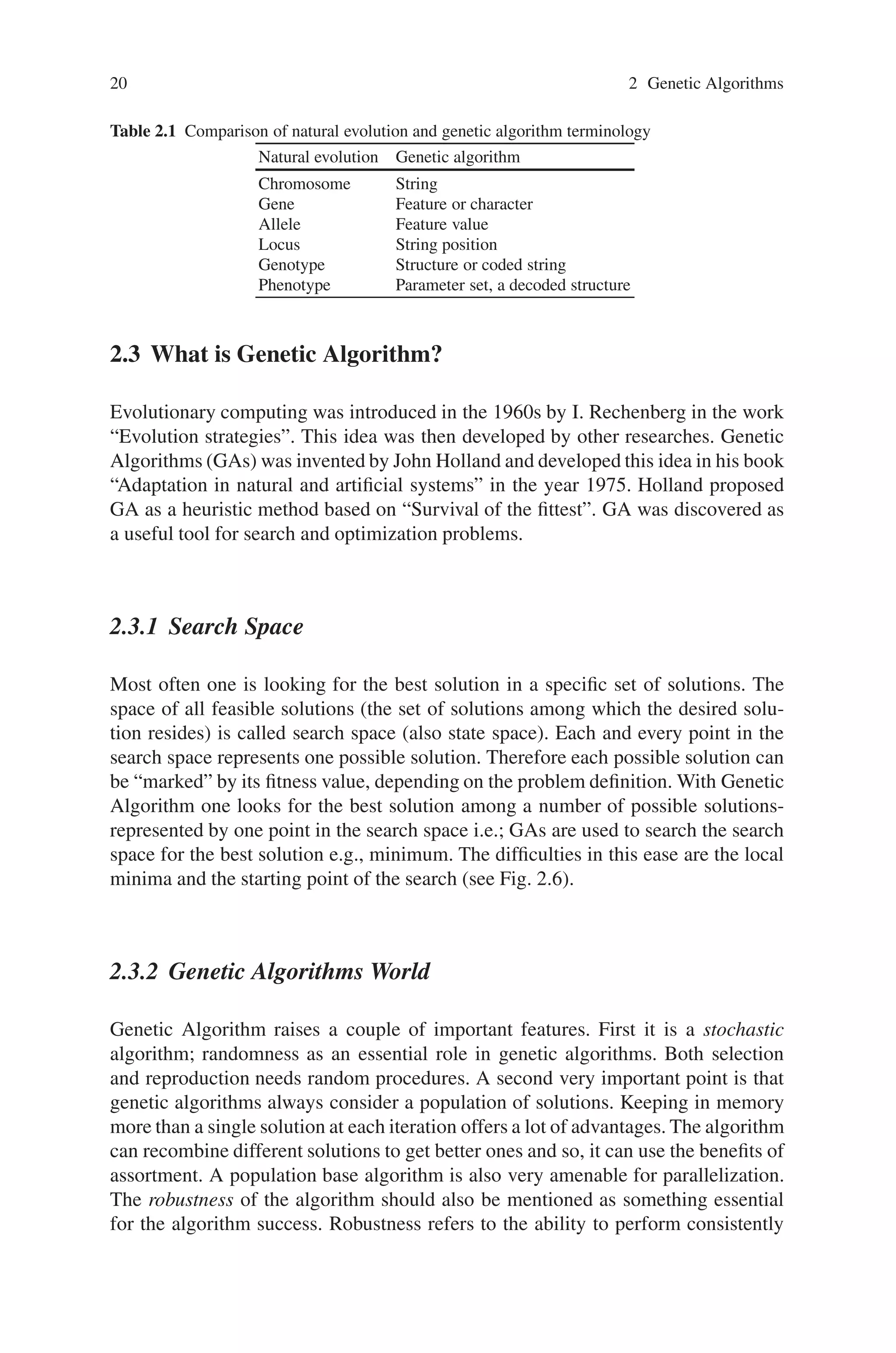
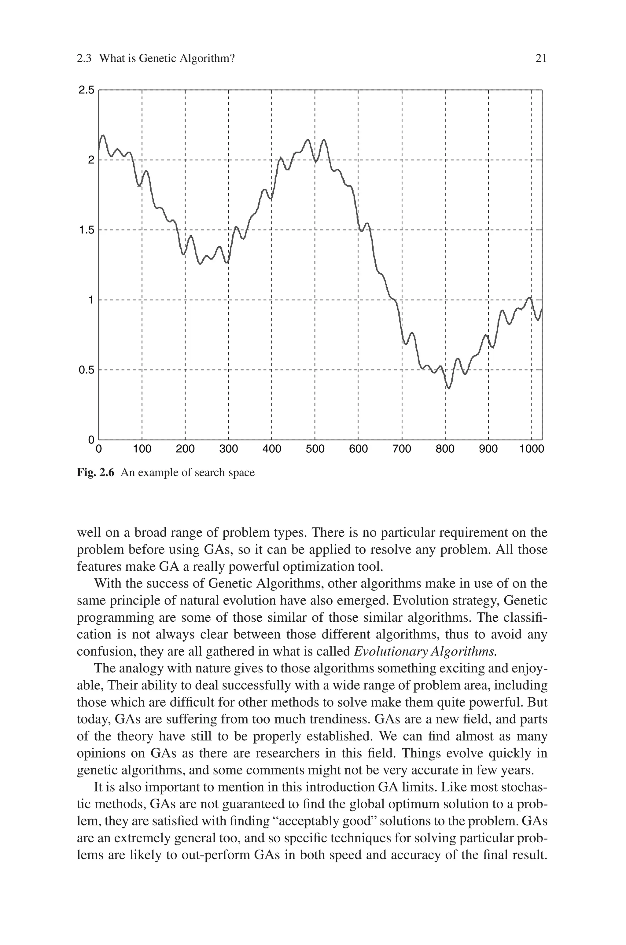
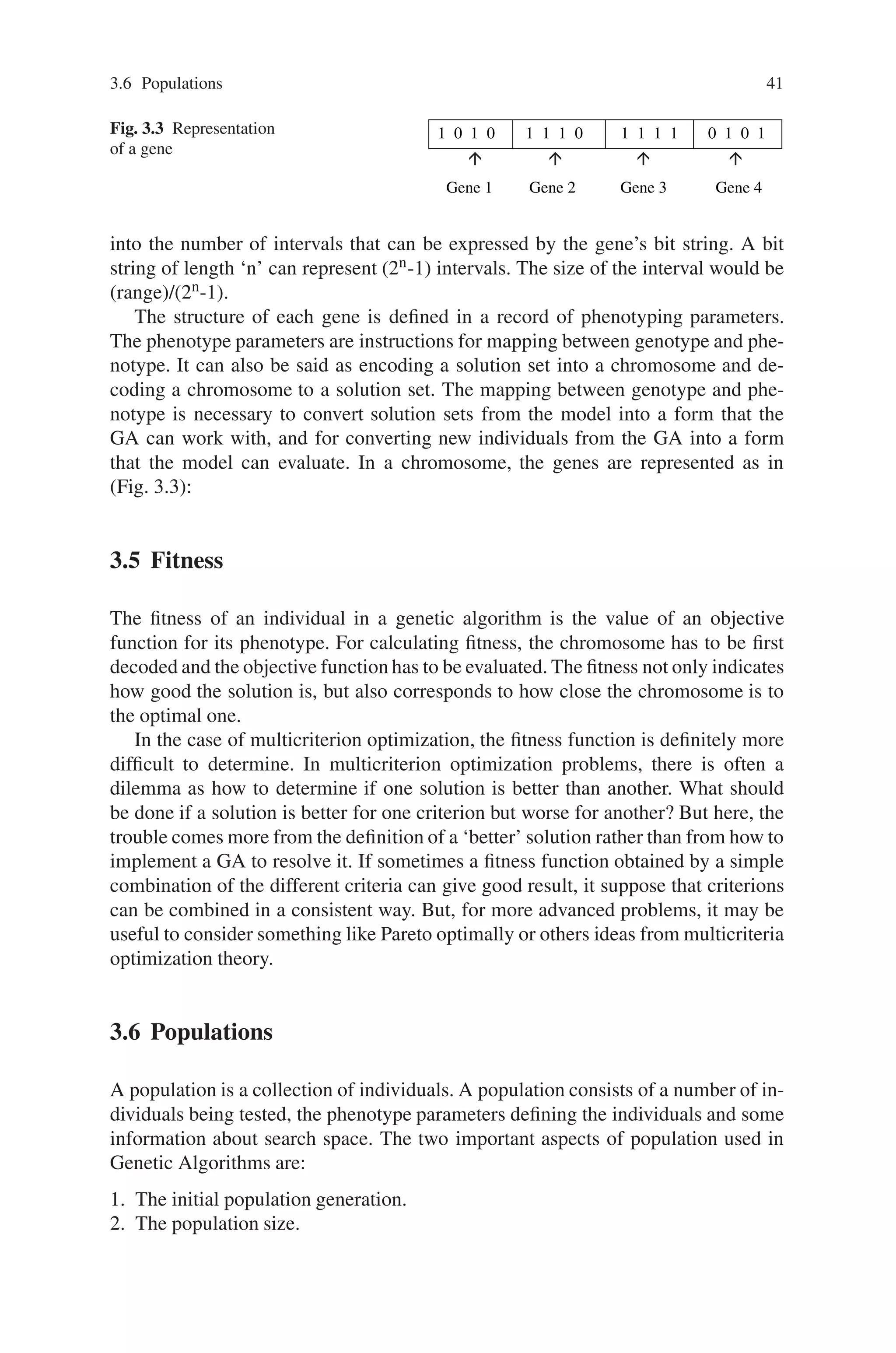
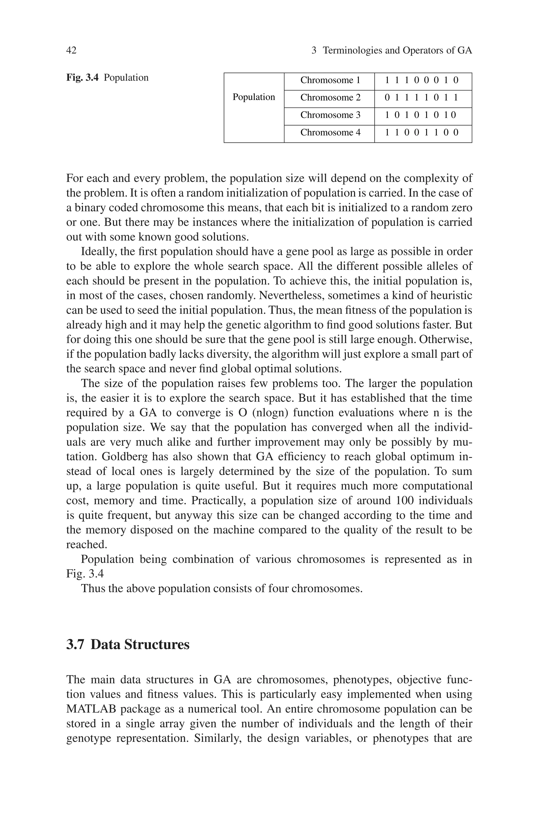
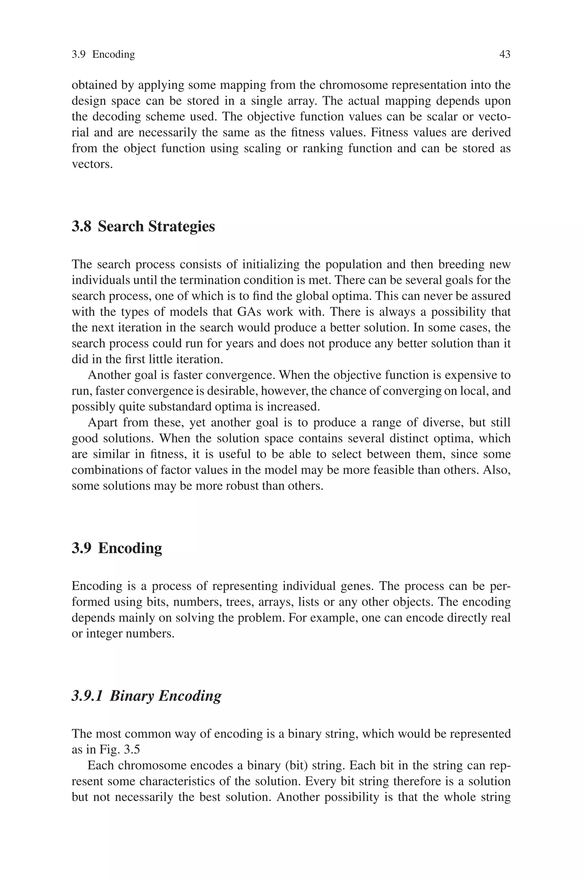
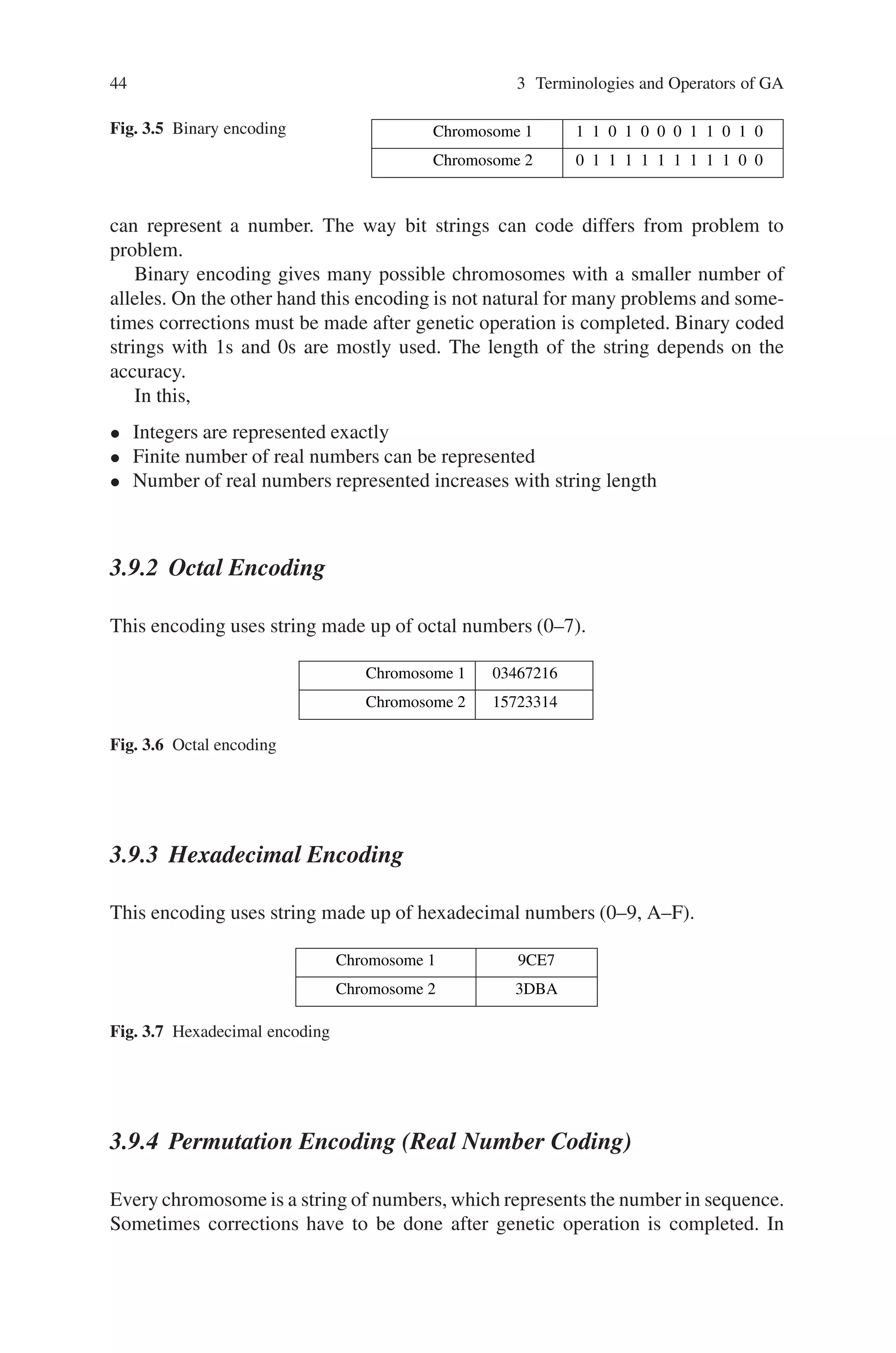
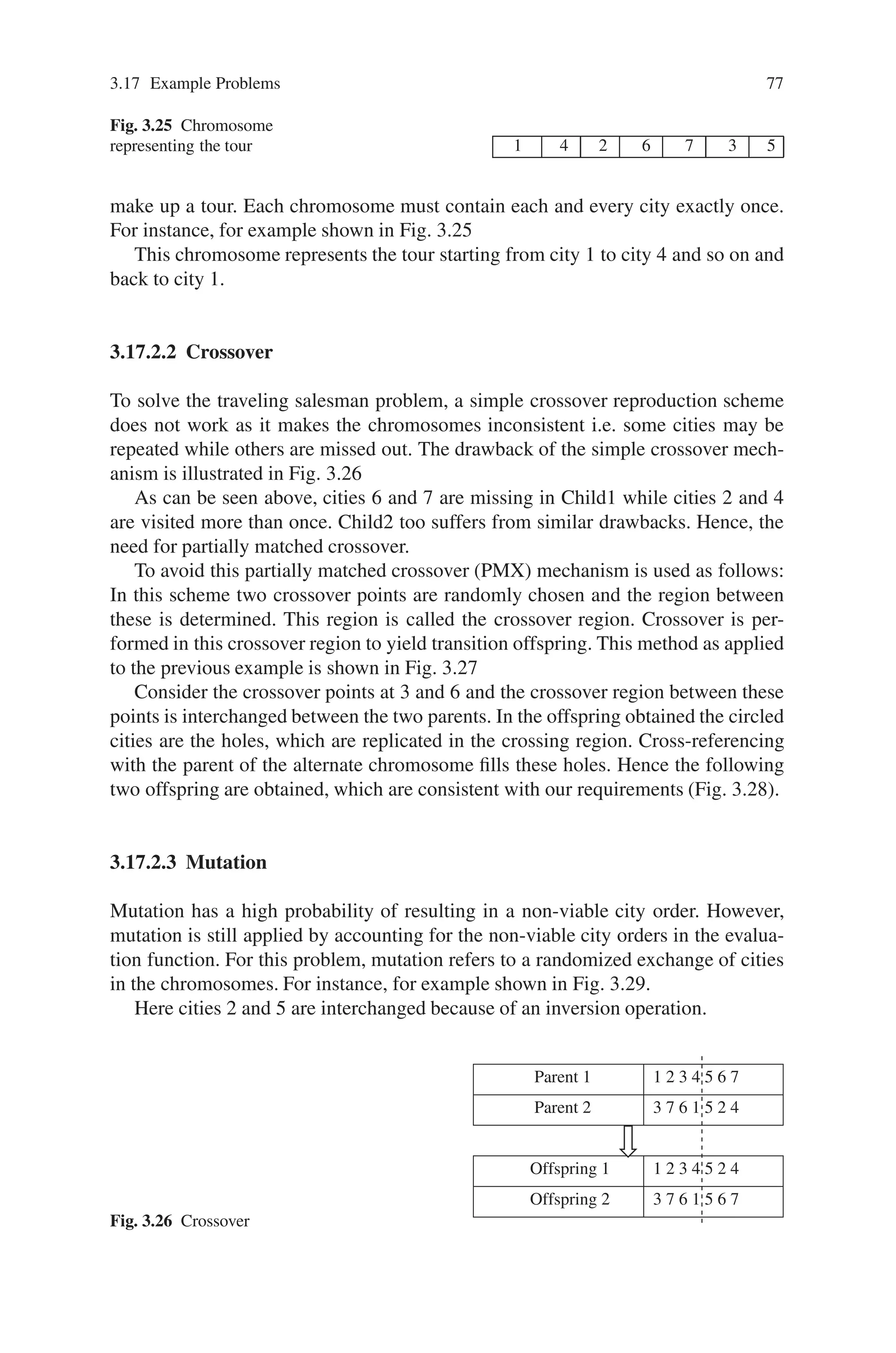
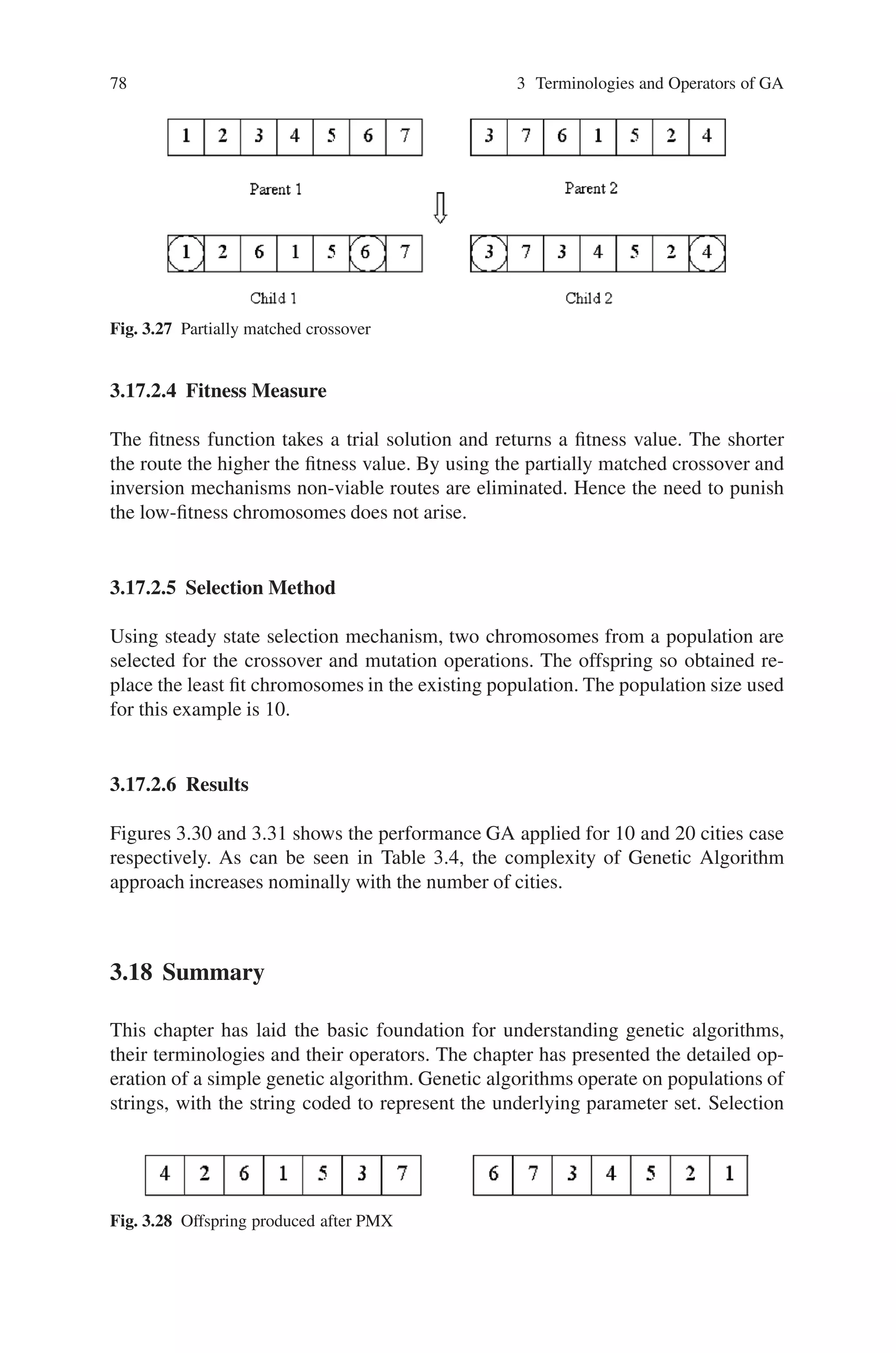
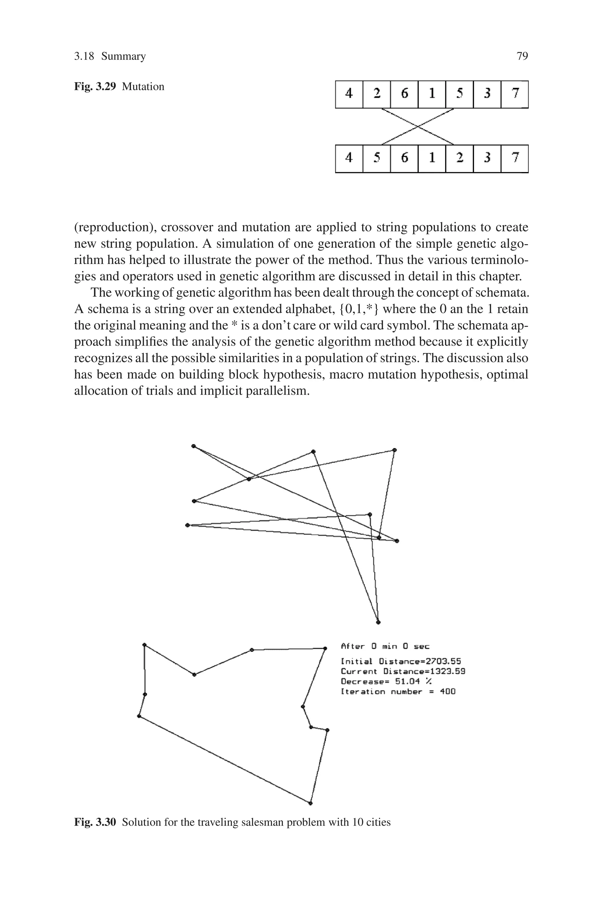
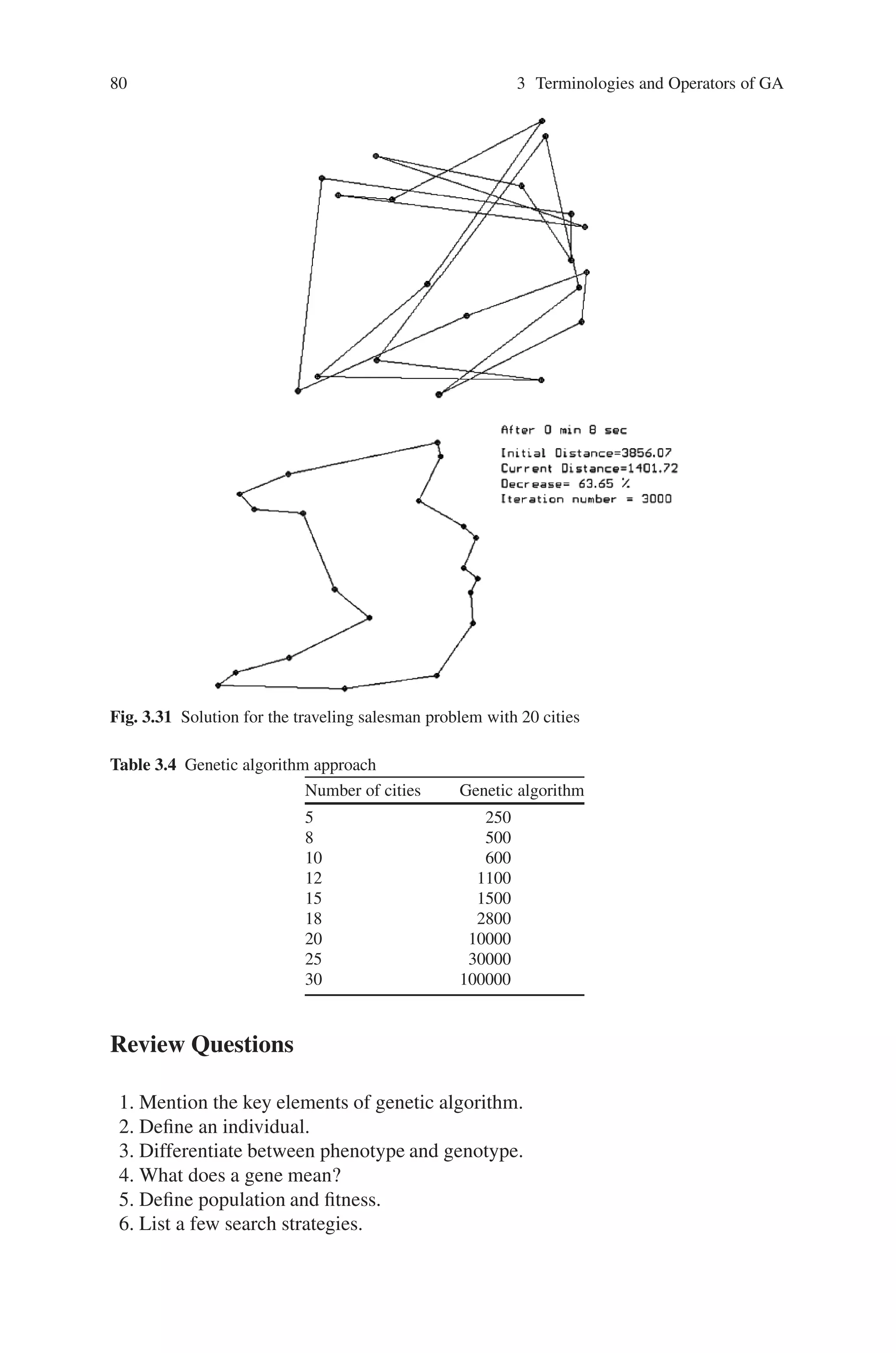
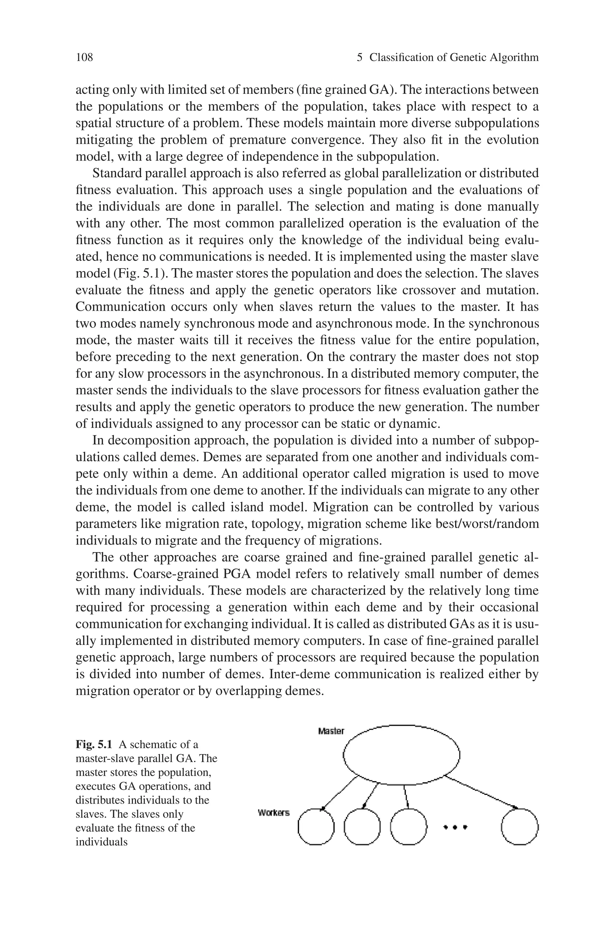
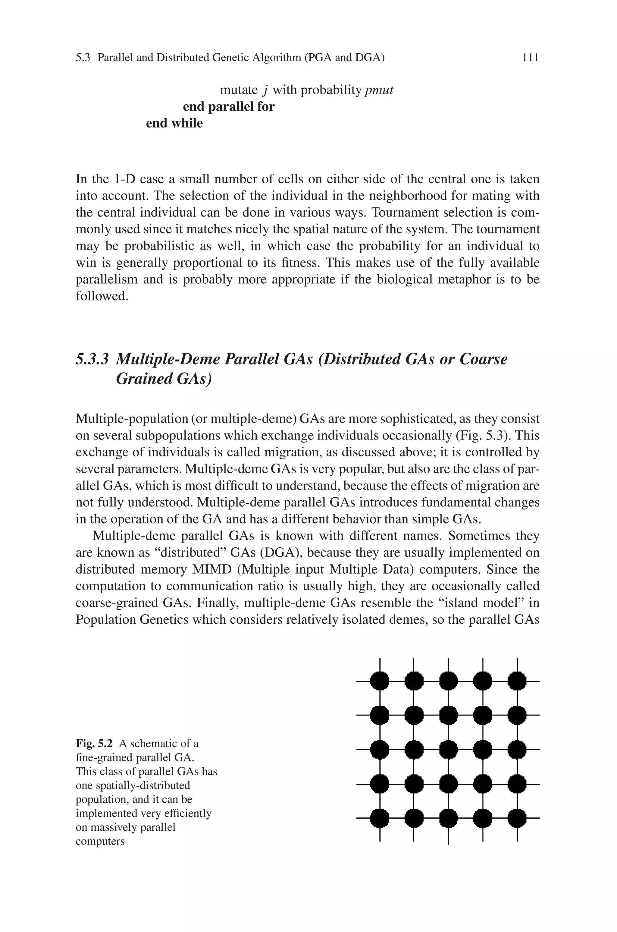
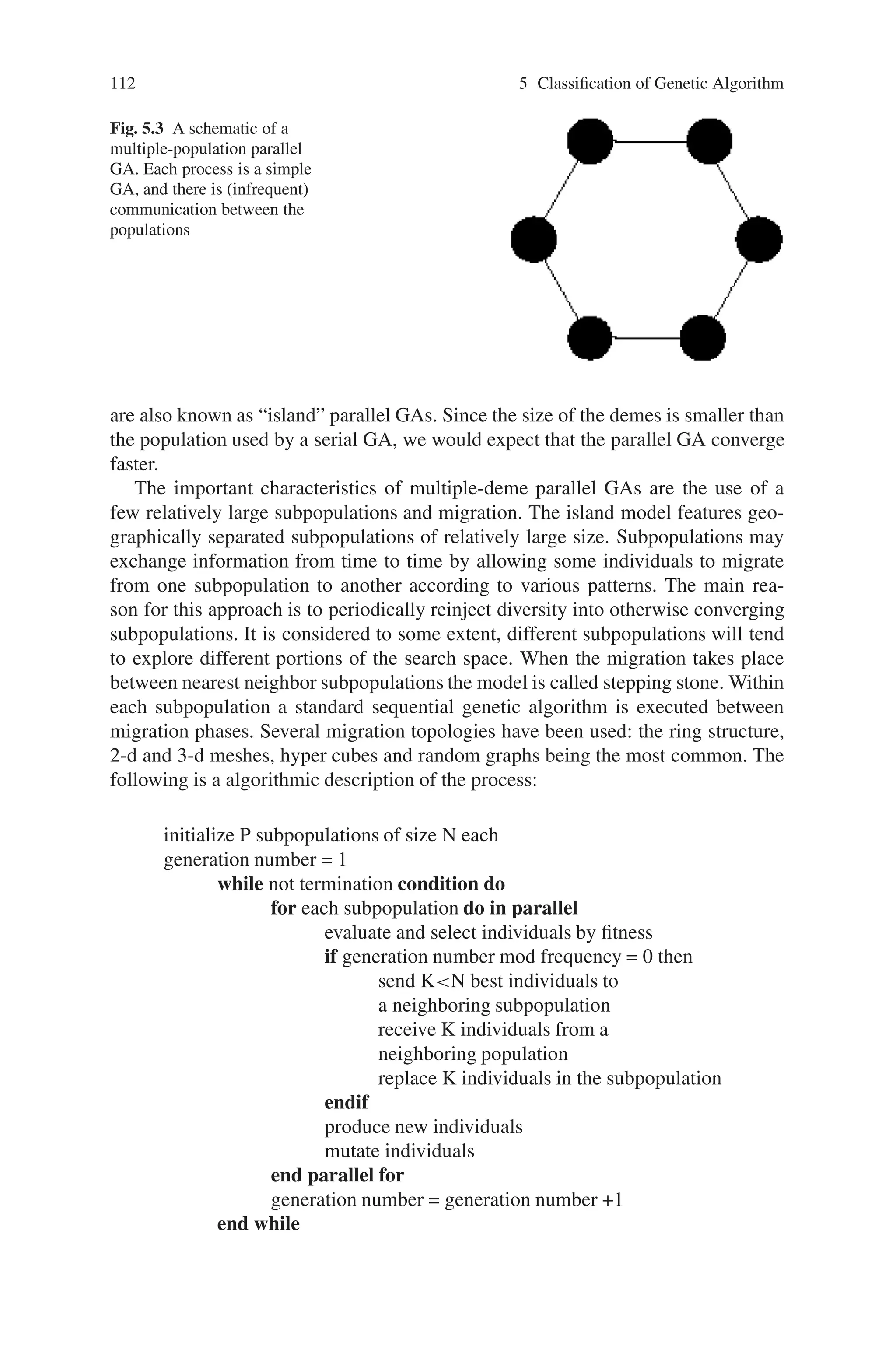
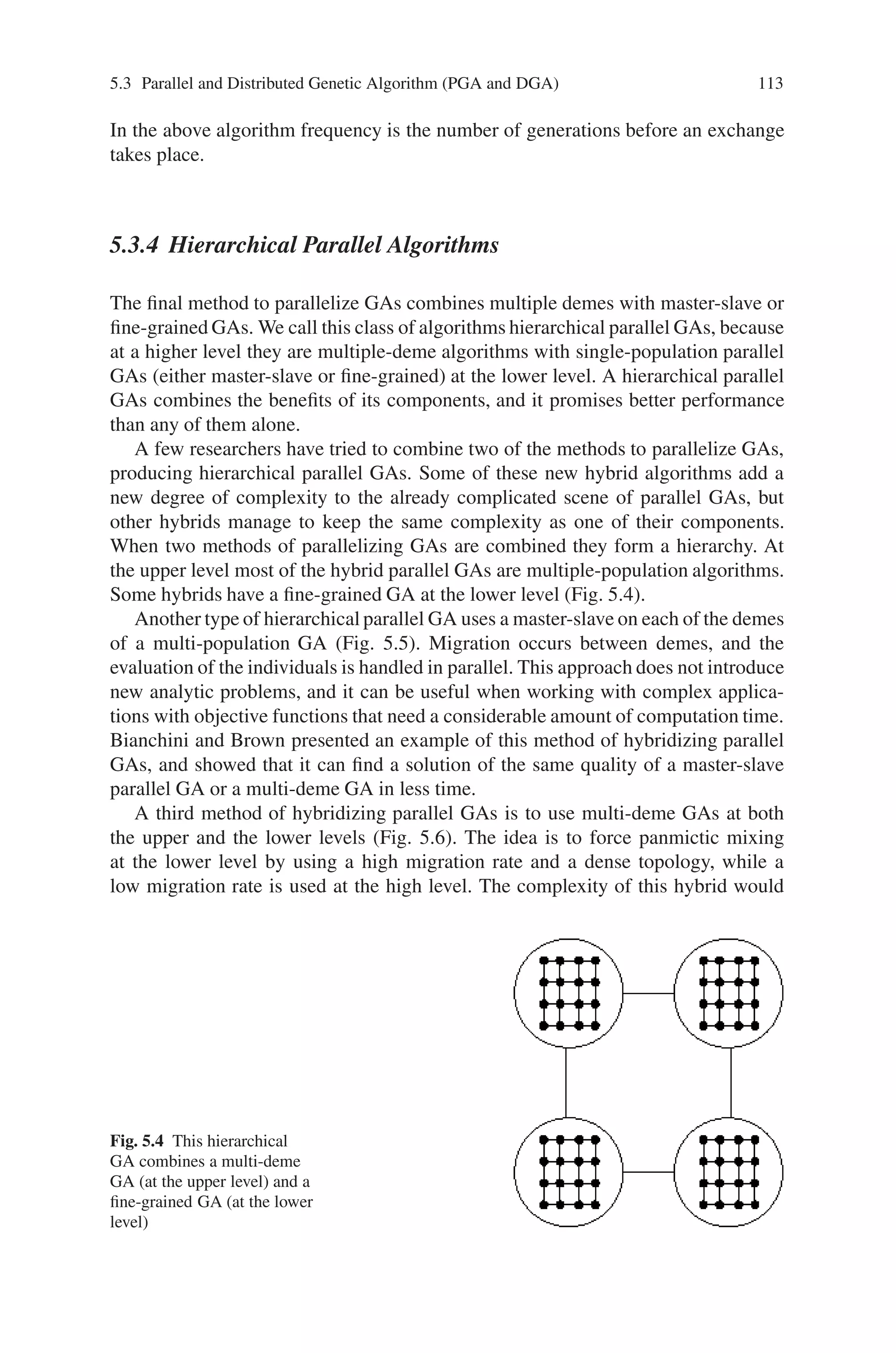
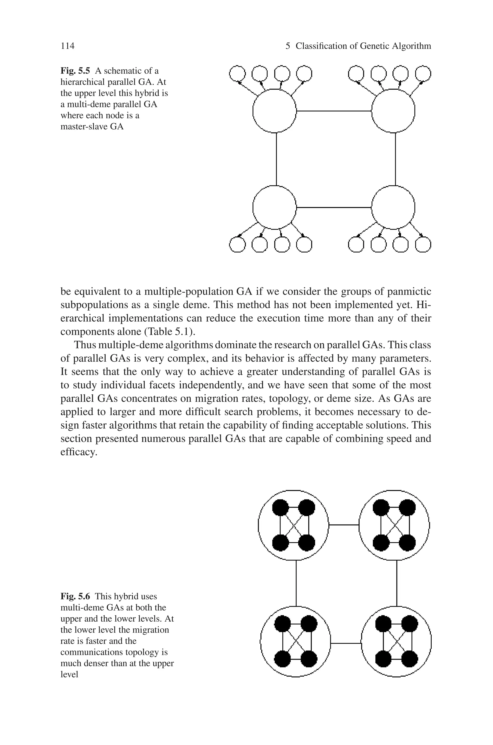
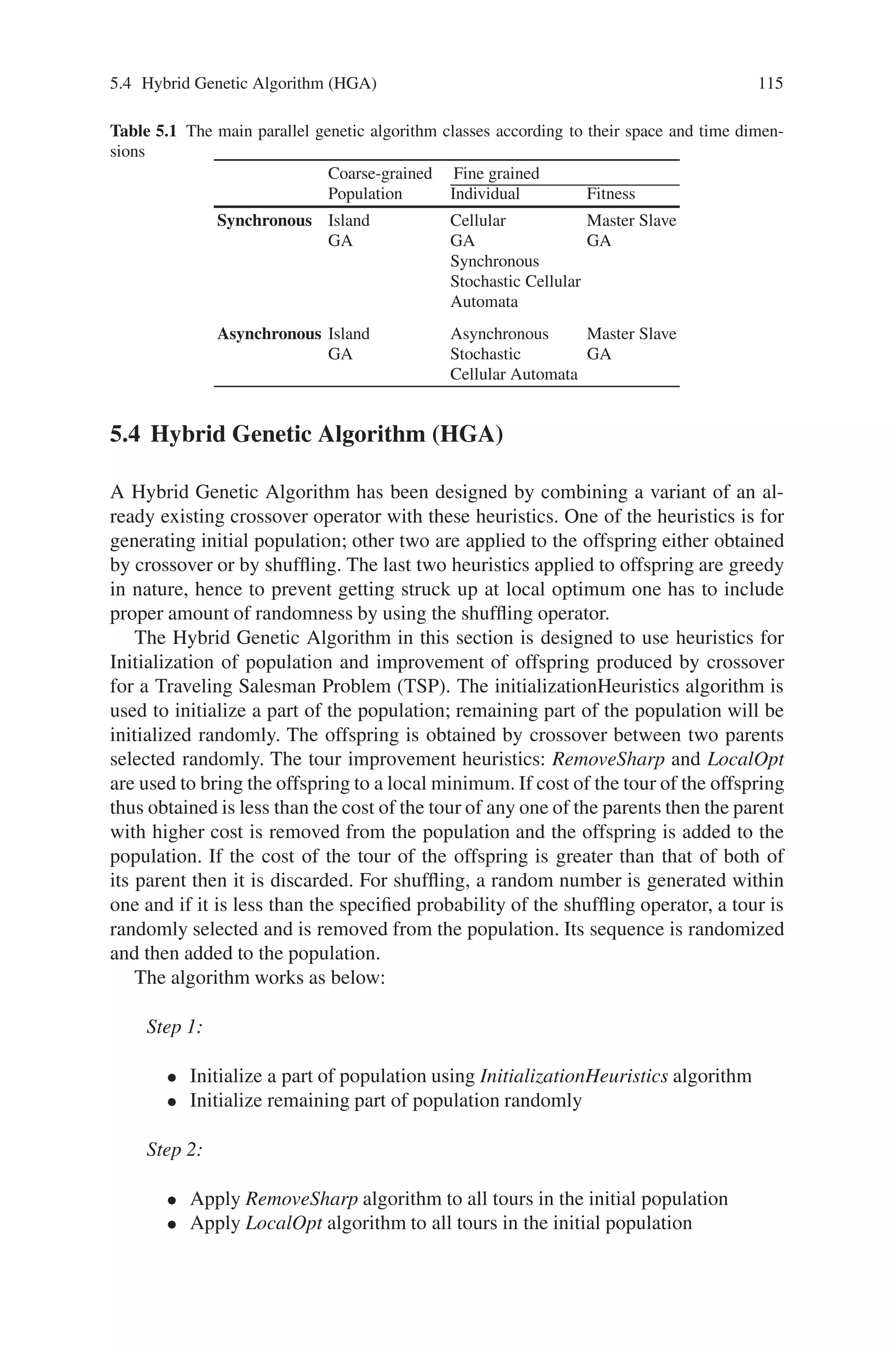
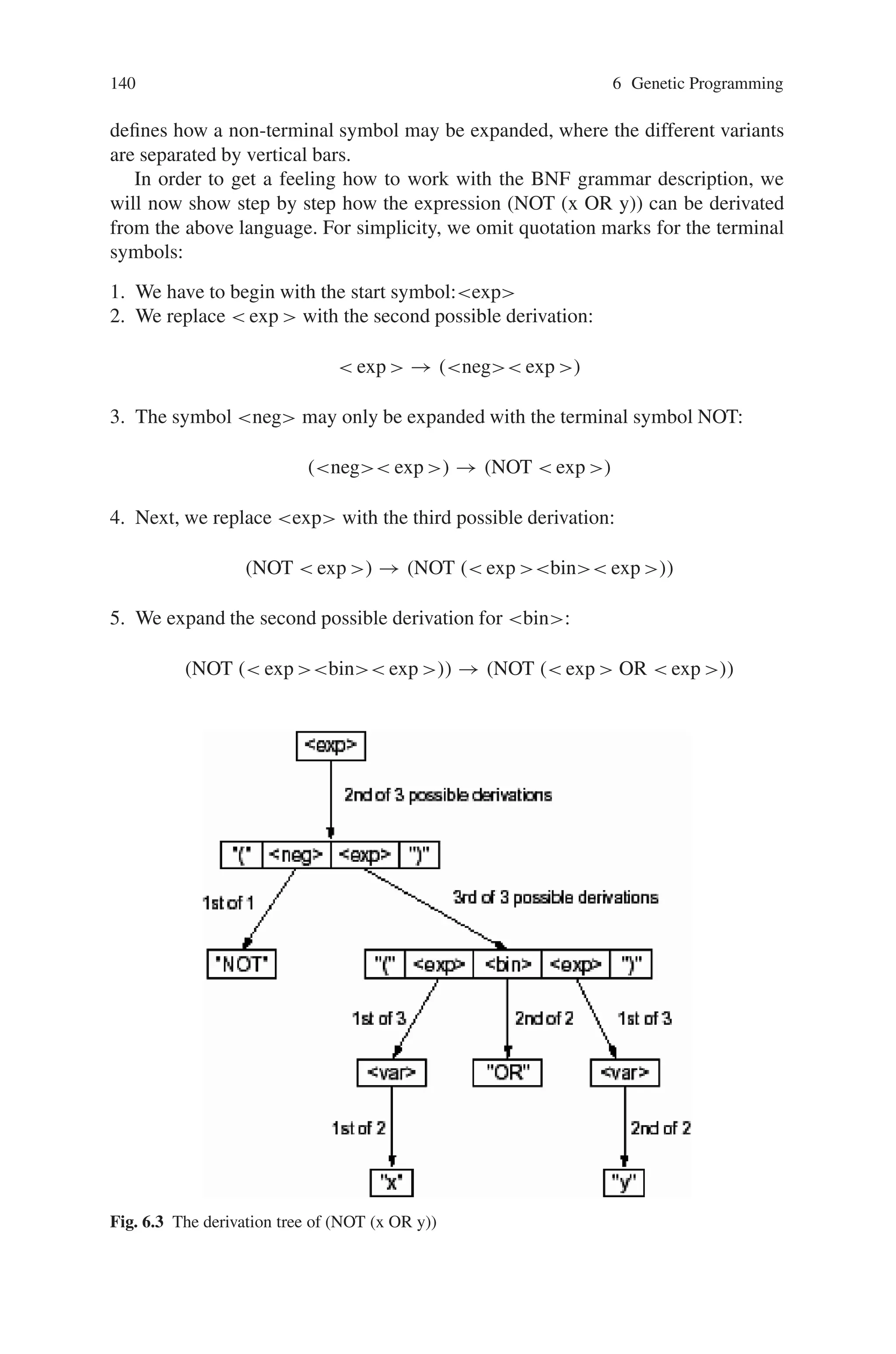
This document provides an introduction to genetic algorithms. It discusses the historical development of evolutionary computation, including genetic algorithms, genetic programming, evolutionary strategies, and evolutionary programming. The key features of evolutionary computation are described, such as particulate genes and population genetics, the adaptive code book, and the genotype/phenotype dichotomy. Advantages of evolutionary computation are highlighted, including conceptual simplicity, broad applicability, hybridization with other methods, parallelism, robustness to dynamic changes, and solving problems with no known solutions. The document concludes with a discussion of applications of evolutionary computation.


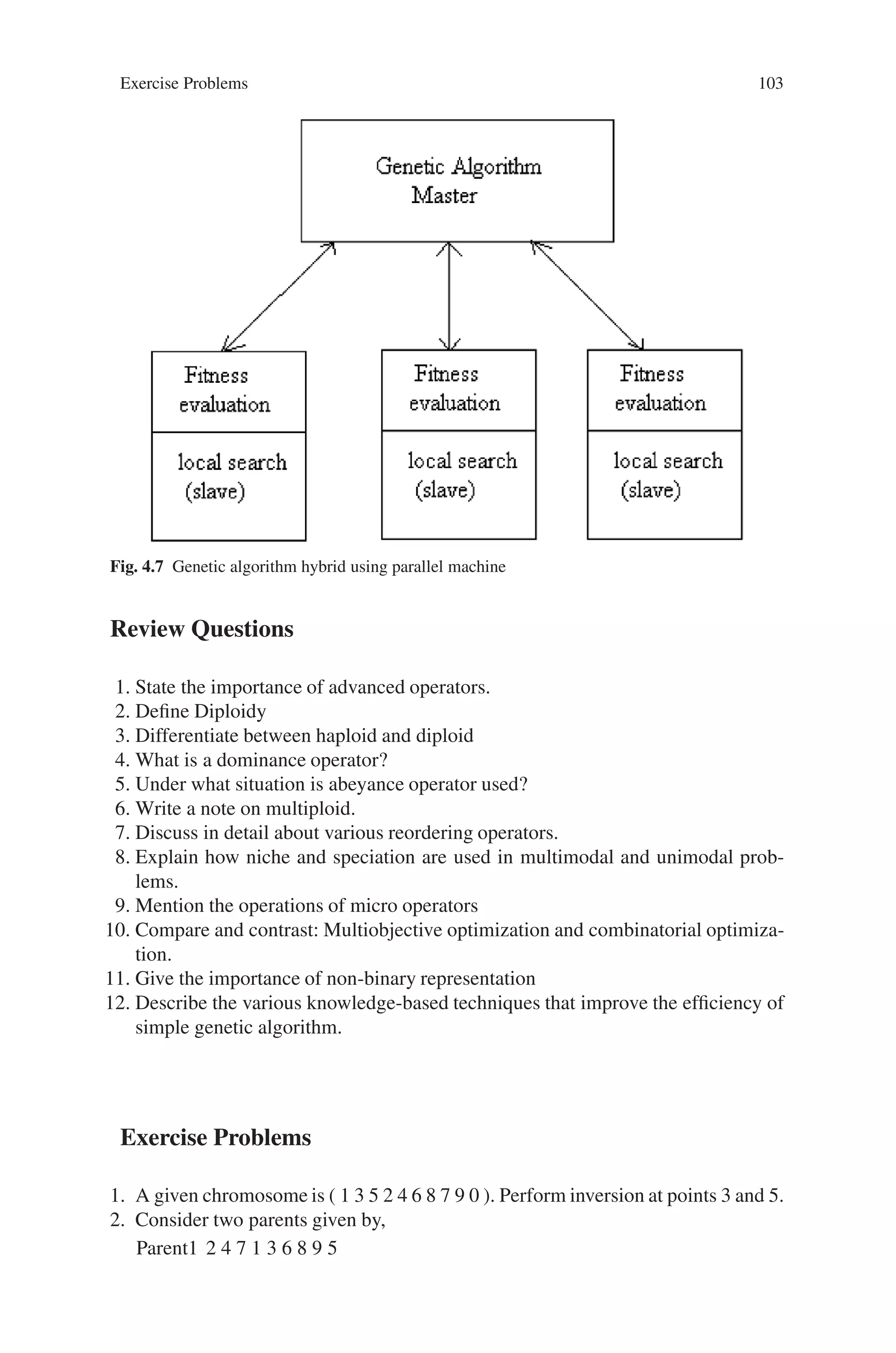
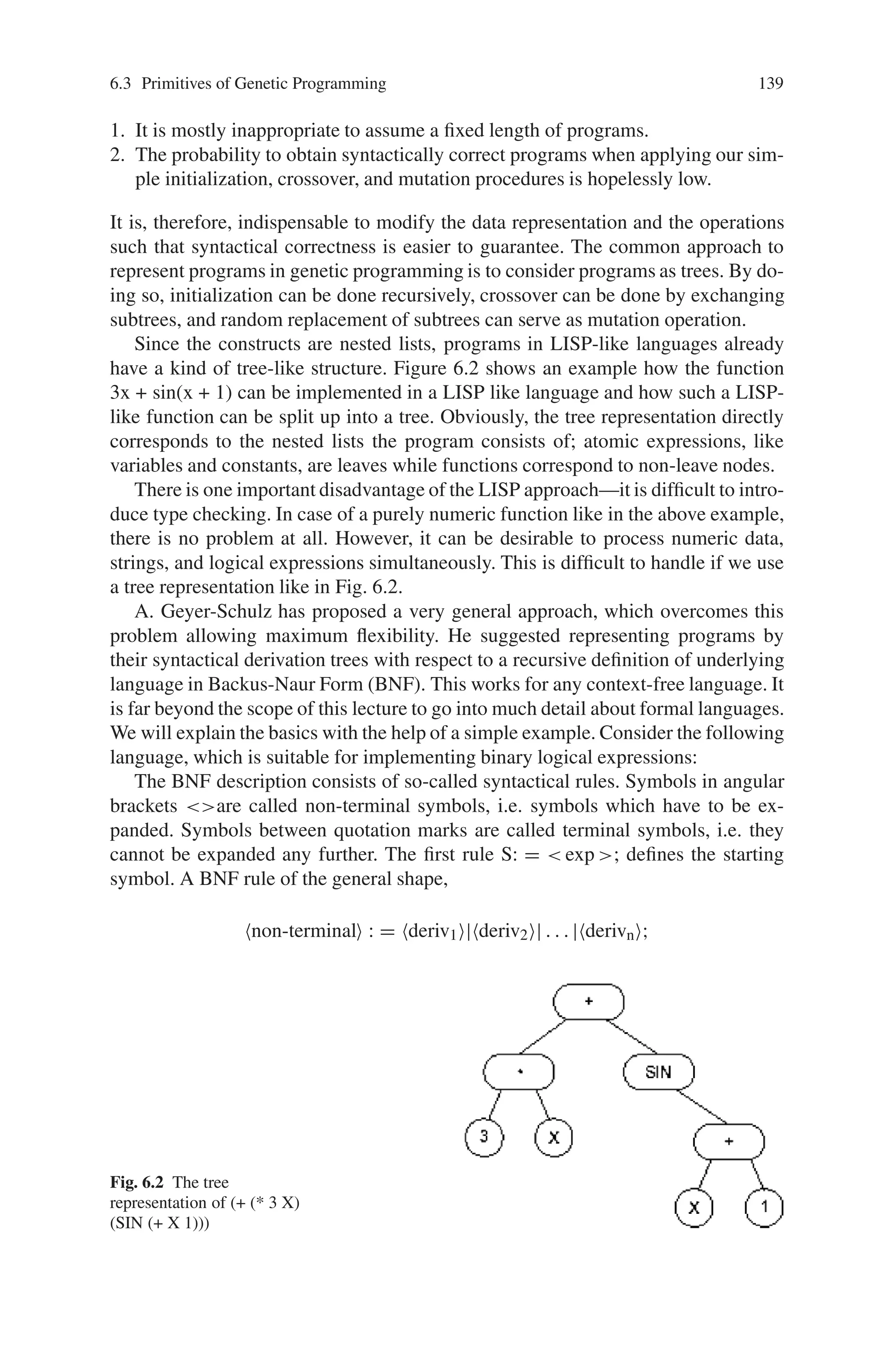
![About the Book ix
in Power System in 1966 from PSG College of Technology, Coimbatore. He
acquired PhD in Control Systems in 1982 from Madras University. He has received
Best Teacher Award in the year 2001 and Dhakshina Murthy Award for Teaching
Excellence from PSG College of Technology. He received The CITATION for best
teaching and technical contribution in the Year 2002, Government College of Tech-
nology, Coimbatore. He has a total teaching experience (UG and PG) of 41 years.
The total number of undergraduateand postgraduate projects guided by him for both
Computer Science and Engineering and Electrical and Electronics Engineering is
around 600. He is currently working as a Professor and Head Computer Science
and Engineering Department, PSG College of Technology, Coimbatore [from June
2000]. He has been identified as an outstanding person in the field of Computer
Science and Engineering in MARQUIS “Who’s Who”, October 2003 issue, New
providence, New Jersey, USA. He has also been identified as an outstanding person
in the field of Computational Science and Engineering in “Who’s Who”, December
2005 issue, Saxe-Coburg Publications, United Kingdom. He has been placed as a
VIP member in the continental WHO’s WHO Registry of national Business Leaders,
Inc. 33 West Hawthorne Avenue Valley Stream, NY 11580, Aug 24, 2006.
S.N. Sivanandam has published 12 books. He has delivered around 150 special
lectures of different specialization in Summer/Winter school and also in various
Engineering colleges. He has guided and coguided 30 Ph.D research works and at
present 9 Ph.D research scholars are working under him. The total number of tech-
nical publications in International/National journals/Conferences is around 700. He
has also received Certificate of Merit 2005–2006 for his paper from The Institution
of Engineers (India). He has chaired 7 International conferences and 30 National
conferences. He is a member of various professional bodies like IE (India), ISTE,
CSI, ACS and SSI. He is a technical advisor for various reputed industries and En-
gineering Institutions. His research areas include Modeling and Simulation, Neural
networks , Fuzzy Systems and Genetic Algorithm, Pattern Recognition, Multi di-
mensional system analysis, Linear and Non linear control system, Signal and Image
processing, Control System, Power system, Numerical methods, Parallel Comput-
ing, Data Mining and Database Security.
S.N. Deepa has completed her B.E Degree from Government College of Technol-
ogy, Coimbatore, 1999 and M.E Degree from PSG College of Technology, Coim-
batore, 2004. She was a gold medalist in her B.E Degree Programme. She has
received G.D Memorial Award in the year 1997 and Best Outgoing Student Award
from PSG College of Technology, 2004. Her M.E Thesis won National Award from
the Indian Society of Technical Education and LT, 2004. She has published 5
books and papers in International and National Journals. Her research areas include
Neural Network, Fuzzy Logic, Genetic Algorithm, Digital Control, Adaptive and
Non-linear Control.](https://image.slidesharecdn.com/s-220425101513/75/S-N-Sivanandam-S-N-Deepa-Introduction-to-Genetic-Algorithms-2008-ISBN-3540731894-pdf-9-2048.jpg)

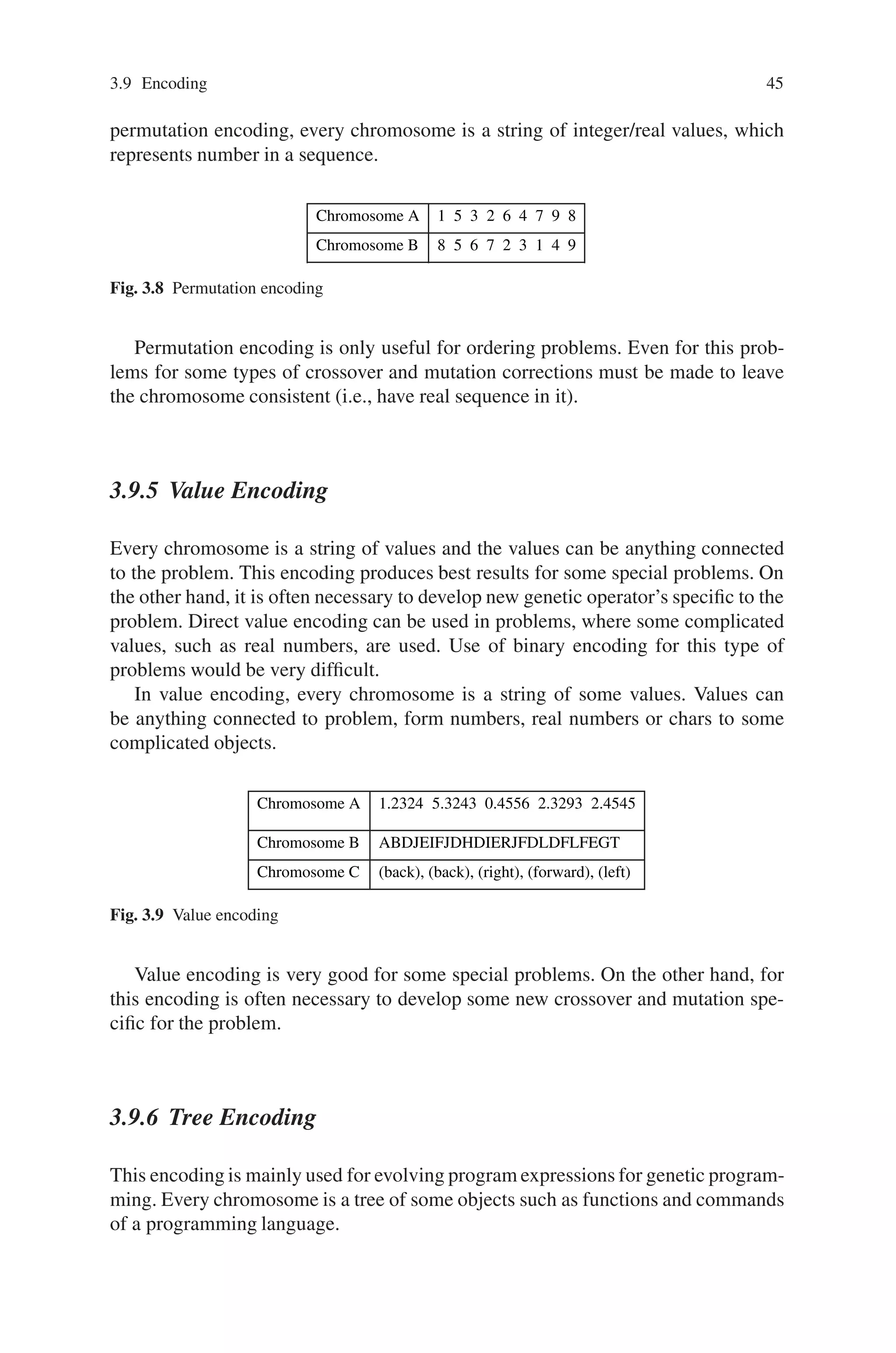
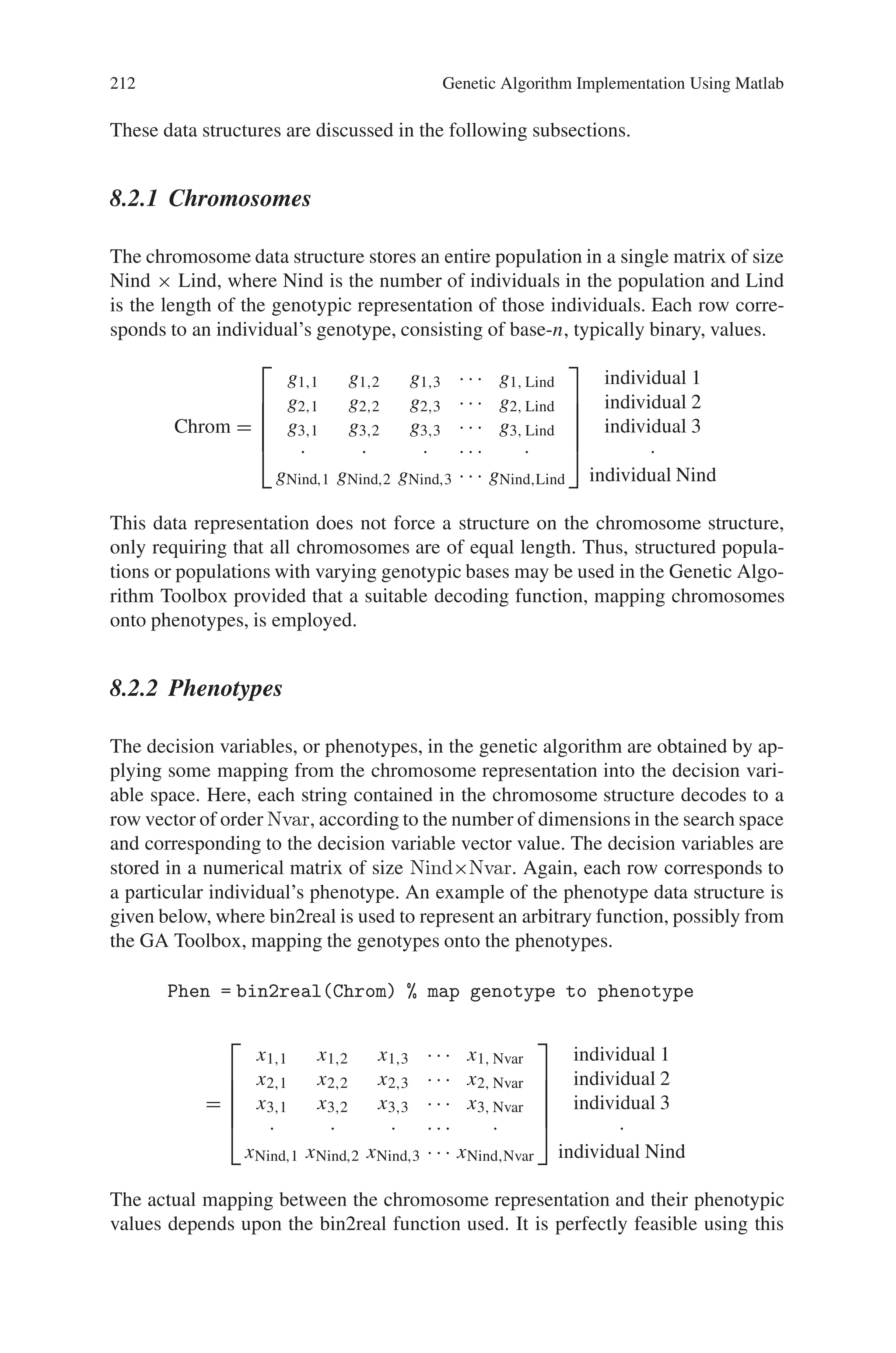
![24 2 Genetic Algorithms
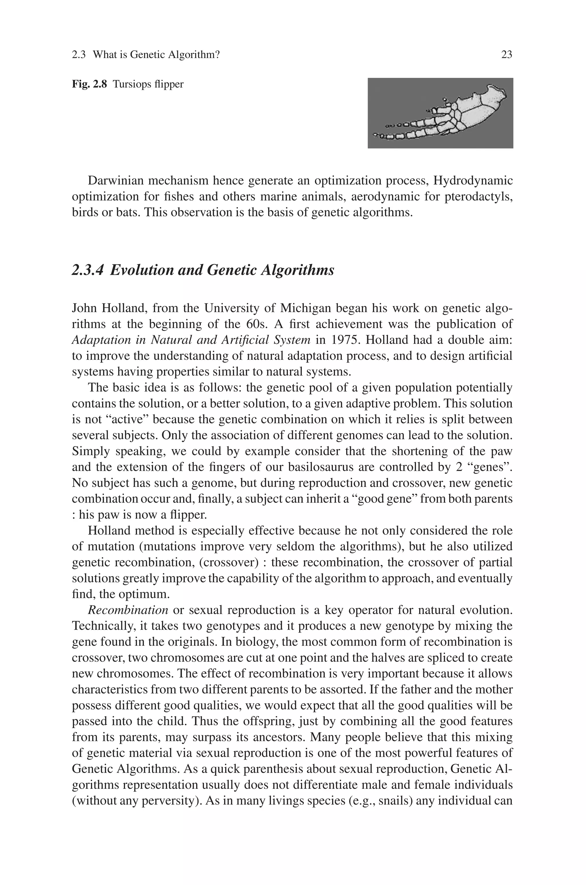
be either a male or a female. In fact, for almost all recombination operators, mother
and father are interchangeable.
Mutation is the other way to get new genomes. Mutation consists in changing
the value of genes. In natural evolution, mutation mostly engenders non-viable
genomes. Actually mutation is not a very frequent operator in natural evolution.
Nevertheless, is optimization, a few random changes can be a good way of exploring
the search space quickly.
Through those low-level notions of genetic, we have seen how living beings
store their characteristic information and how this information can be passed into
their offspring. It very basic but it is more than enough to understand the Genetic
Algorithm Theory.
Darwin was totally unaware of the biochemical basics of genetics. Now we know
how the genetic inheritable information is coded in DNA, RNA and proteins and that
the coding principles are actually digital much resembling the information storage in
computers. Information processing is in many ways totally different, however. The
magnificent phenomenon called the evolution of species can also give some insight
into information processing methods and optimization in particular. According to
Darwinism, inherited variation is characterized by the following properties:
1. Variation must be copying because selection does not create directly anything,
but presupposes a large population to work on.
2. Variation must be small-scaled in practice. Species do not appear suddenly.
3. Variation is undirected. This is also known as the blind watchmaker paradigm.
While the natural sciences approach to evolution has for over a century been to
analyze and study different aspects of evolution to find the underlying principles,
the engineering sciences are happy to apply evolutionary principles, that have been
heavily tested over billions of years, to attack the most complex technical problems,
including protein folding.
2.4 Conventional Optimization and Search Techniques
The basic principle of optimization is the efficient allocation of scarce resources.
Optimization can be applied to any scientific or engineering discipline. The aim
of optimization is to find an algorithm, which solves a given class of problems.
There exist no specific method, which solves all optimization problems. Consider a
function,
f(x):
xl
, xu
→ [0, 1] : (2.1)
where,
f (x) =
1, i f ||x − a|| ∈, ∈ 0
−1, elsewhere](https://image.slidesharecdn.com/s-220425101513/75/S-N-Sivanandam-S-N-Deepa-Introduction-to-Genetic-Algorithms-2008-ISBN-3540731894-pdf-40-2048.jpg)
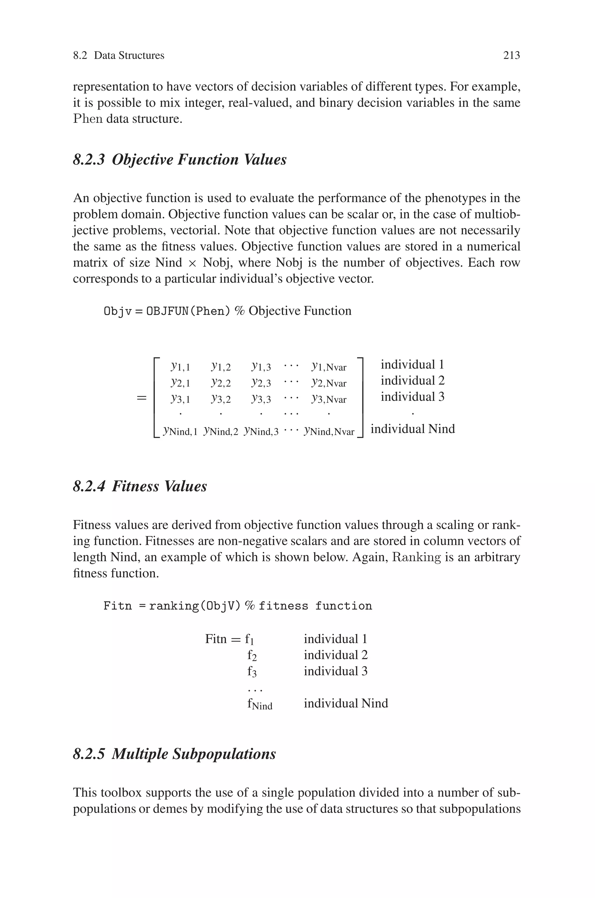
![2.4 Conventional Optimization and Search Techniques 25
For the above function, f can be maintained by decreasing € or by making the inter-
val of [ xl, xu ] large. Thus a difficult task can be made easier. Therefore, one can
solve optimization problems by combining human creativity and the raw processing
power of the computers.
The various conventional optimization and search techniques available are dis-
cussed as follows:
2.4.1 Gradient-Based Local Optimization Method
When the objective function is smooth and one need efficient local optimization, it
is better to use gradient based or Hessian based optimization methods. The perfor-
mance and reliability of the different gradient methods varies considerably.
To discuss gradient-based local optimization, let us assume a smooth objective
function (i.e., continuous first and second derivatives). The objective function is
denoted by,
f(x): Rn
→ R (2.2)
The first derivatives are contained in the gradient vector ∇ f(x)
∇ f (x) =
⎡
⎢
⎣
∂ f (x)/∂x1
.
.
.
∂ f (x)/∂xn
⎤
⎥
⎦ (2.3)
The second derivatives of the objective function are contained in the Hessian matrix
H(x).
H(x) = ∇T
∇ f (x) =
⎛
⎜
⎜
⎜
⎝
∂2 f (x)
∂2x1
· · · ∂2 f (x)
∂x1∂xn
.
.
.
.
.
.
∂2 f (x)
∂x1∂xn
· · · ∂2 f (x)
∂2xn
⎞
⎟
⎟
⎟
⎠
(2.4)
Few methods need only the gradient vector, but in the Newton’s method we need
the Hessian matrix.
The general pseudo code used in gradient methods is as follows:
Select an initial guess value xl and set n=1.
repeat
Solve the search direction pn from (2.5) or (2.6) below.
Determine the next iteration point using (2.7) below:
Xn+1 = Xn + λnPn
Set n=n+1.
Until ||Xn − Xn−1|| ∈](https://image.slidesharecdn.com/s-220425101513/75/S-N-Sivanandam-S-N-Deepa-Introduction-to-Genetic-Algorithms-2008-ISBN-3540731894-pdf-41-2048.jpg)
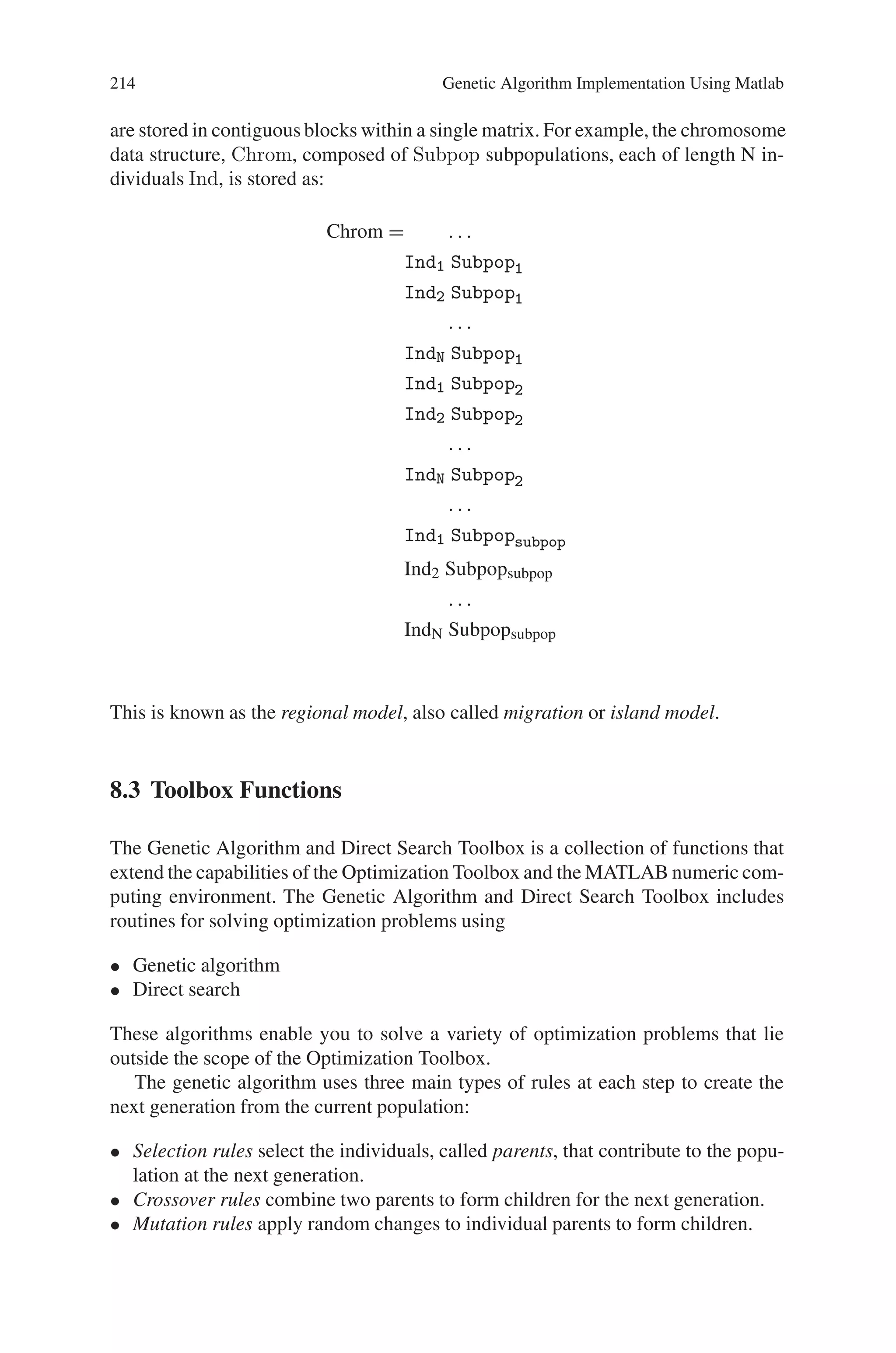
![30 2 Genetic Algorithms
Selection is supposed to be able to compare each individual in the population.
Selection is done by using a fitness function. Each chromosome has an associated
value corresponding to the fitness of the solution it represents. The fitness should
correspond to an evaluation of how good the candidate solution is. The optimal
solution is the one, which maximizes the fitness function. Genetic Algorithms deal
with the problems that maximize the fitness function. But, if the problem consists
in minimizing a cost function, the adaptation is quite easy. Either the cost function
can be transformed into a fitness function, for example by inverting it; or the selec-
tion can be adapted in such way that they consider individuals with low evaluation
functions as better.
Once the reproduction and the fitness function have been properly defined, a
Genetic Algorithm is evolved according to the same basic structure. It starts by
generating an initial population of chromosomes. This first population must offer
a wide diversity of genetic materials. The gene pool should be as large as possible
so that any solution of the search space can be engendered. Generally, the initial
population is generated randomly.
Then, the genetic algorithm loops over an iteration process to make the popula-
tion evolve. Each iteration consists of the following steps:
• SELECTION: The first step consists in selecting individuals for reproduction.
This selection is done randomly with a probability depending on the relative
fitness of the individuals so that best ones are often chosen for reproduction than
poor ones.
• REPRODUCTION: In the second step, offspring are bred by the selected indi-
viduals. For generating new chromosomes, the algorithm can use both recombi-
nation and mutation.
• EVALUATION: Then the fitness of the new chromosomes is evaluated.
• REPLACEMENT: During the last step, individuals from the old population are
killed and replaced by the new ones.
The algorithm is stopped when the population convergestoward the optimal solution.
The basic genetic algorithm is as follows:
• [start] Genetic random population of n chromosomes (suitable solutions for the
problem)
• [Fitness] Evaluate the fitness f(x) of each chromosome x in the population
• New population] Create a new population by repeating following steps until the
New population is complete
- [selection] select two parent chromosomes from a population according to
their fitness ( the better fitness, the bigger chance to get selected).
- [crossover] With a crossover probability, cross over the parents to form new
offspring ( children). If no crossover was performed, offspring is the exact
copy of parents.
- [Mutation] With a mutation probability, mutate new offspring at each locus
(position in chromosome)
- [Accepting] Place new offspring in the new population.](https://image.slidesharecdn.com/s-220425101513/75/S-N-Sivanandam-S-N-Deepa-Introduction-to-Genetic-Algorithms-2008-ISBN-3540731894-pdf-46-2048.jpg)
![2.5 A Simple Genetic Algorithm 31
• [Replace] Use new generated population for a further sum of the algorithm.
• [Test] If the end condition is satisfied, stop, and return the best solution in current
population.
• [Loop] Go to step2 for fitness evaluation.
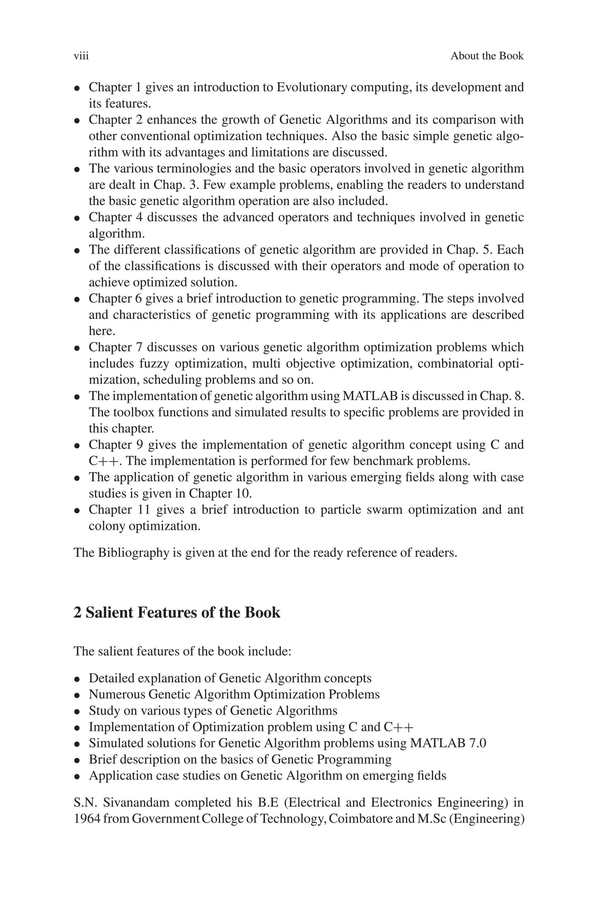
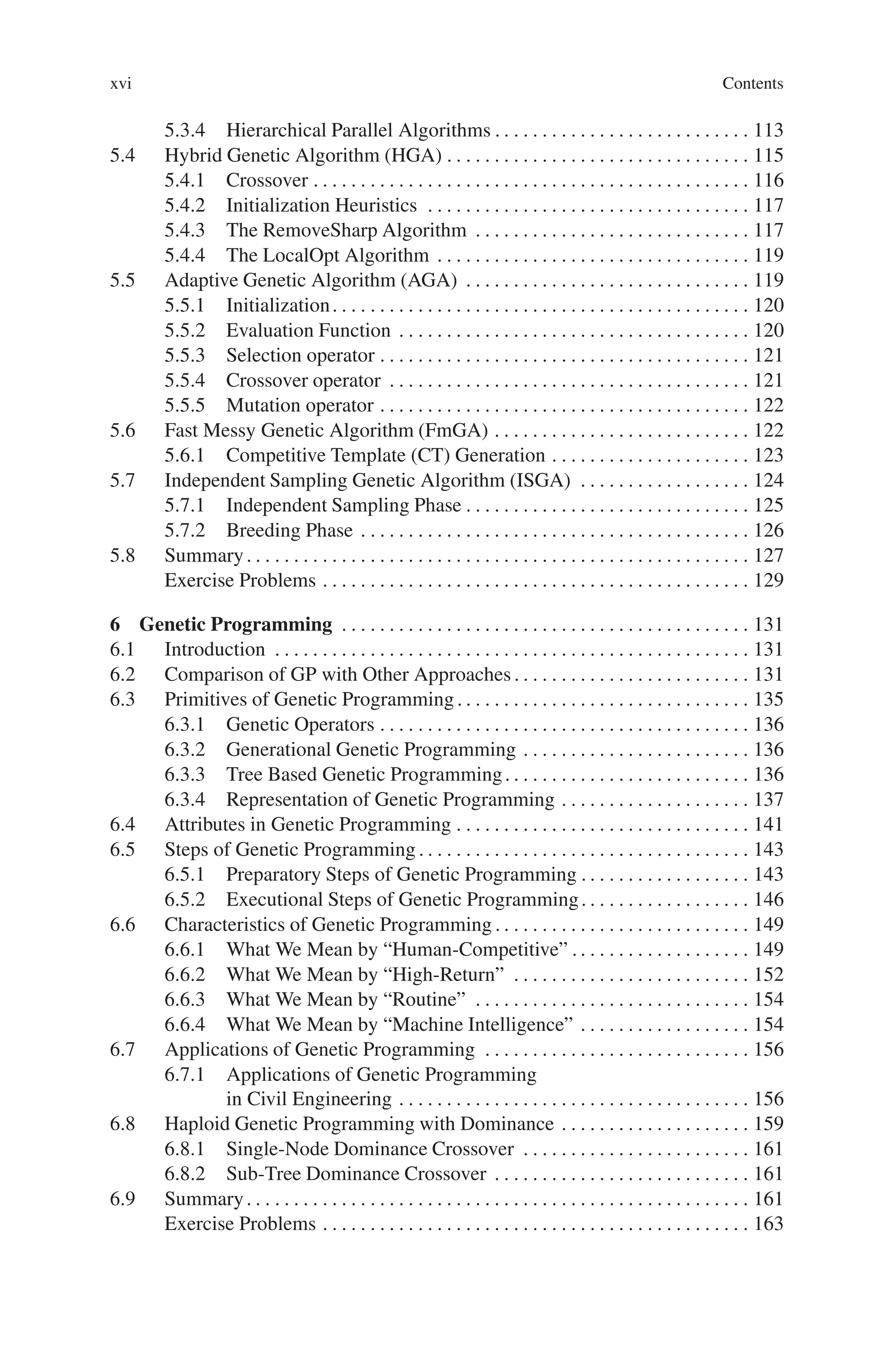
The Genetic algorithm process is discussed through the GA cycle in Fig. 2.9
Reproduction is the process by which the genetic material in two or more parent
is combined to obtain one or more offspring. In fitness evaluation step, the indi-
vidual’s quality is assessed. Mutation is performed to one individual to produce a
new version of it where some of the original genetic material has been randomly
changed. Selection process helps to decide which individuals are to be used for
reproduction and mutation in order to produce new search points.
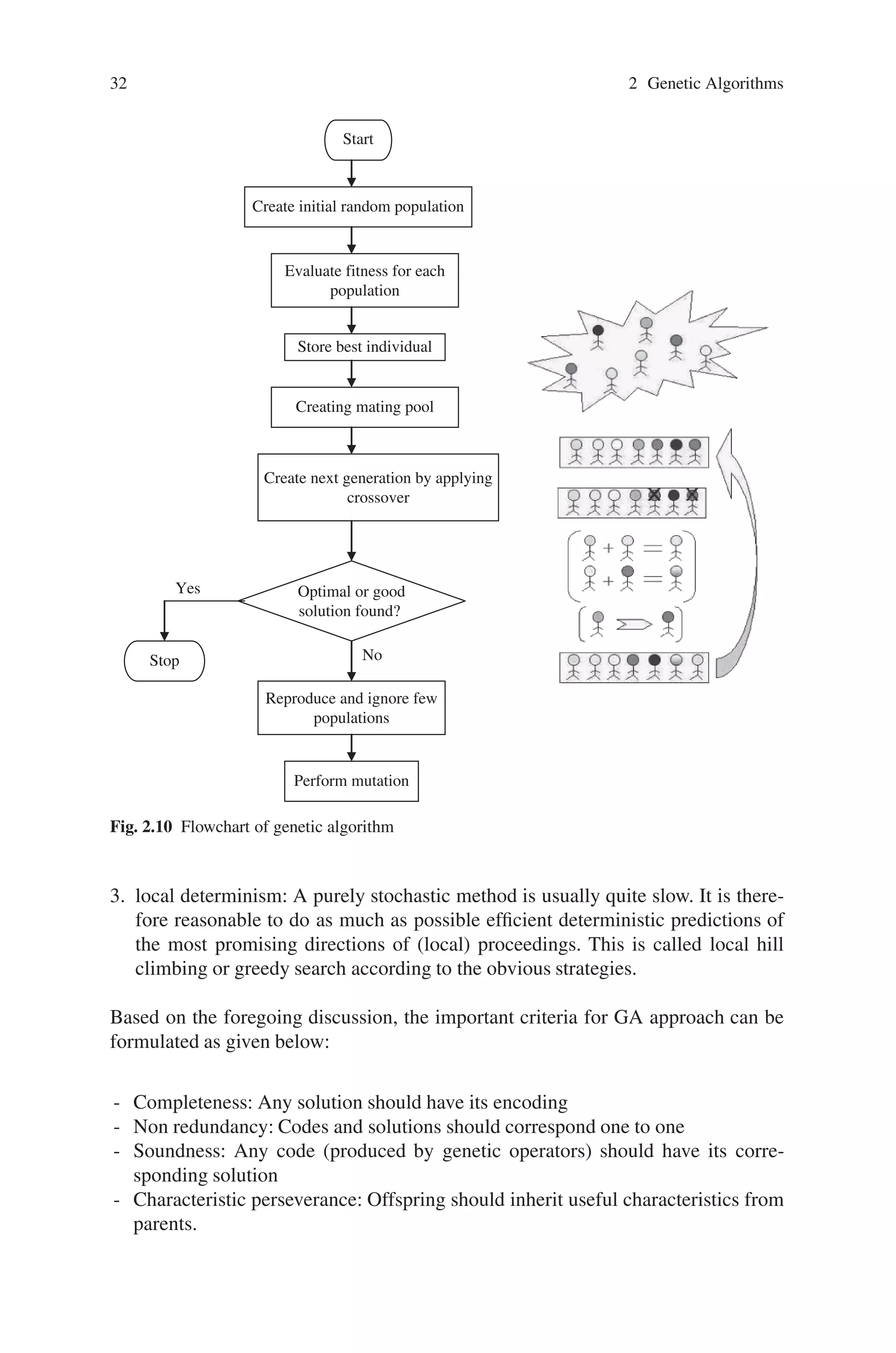
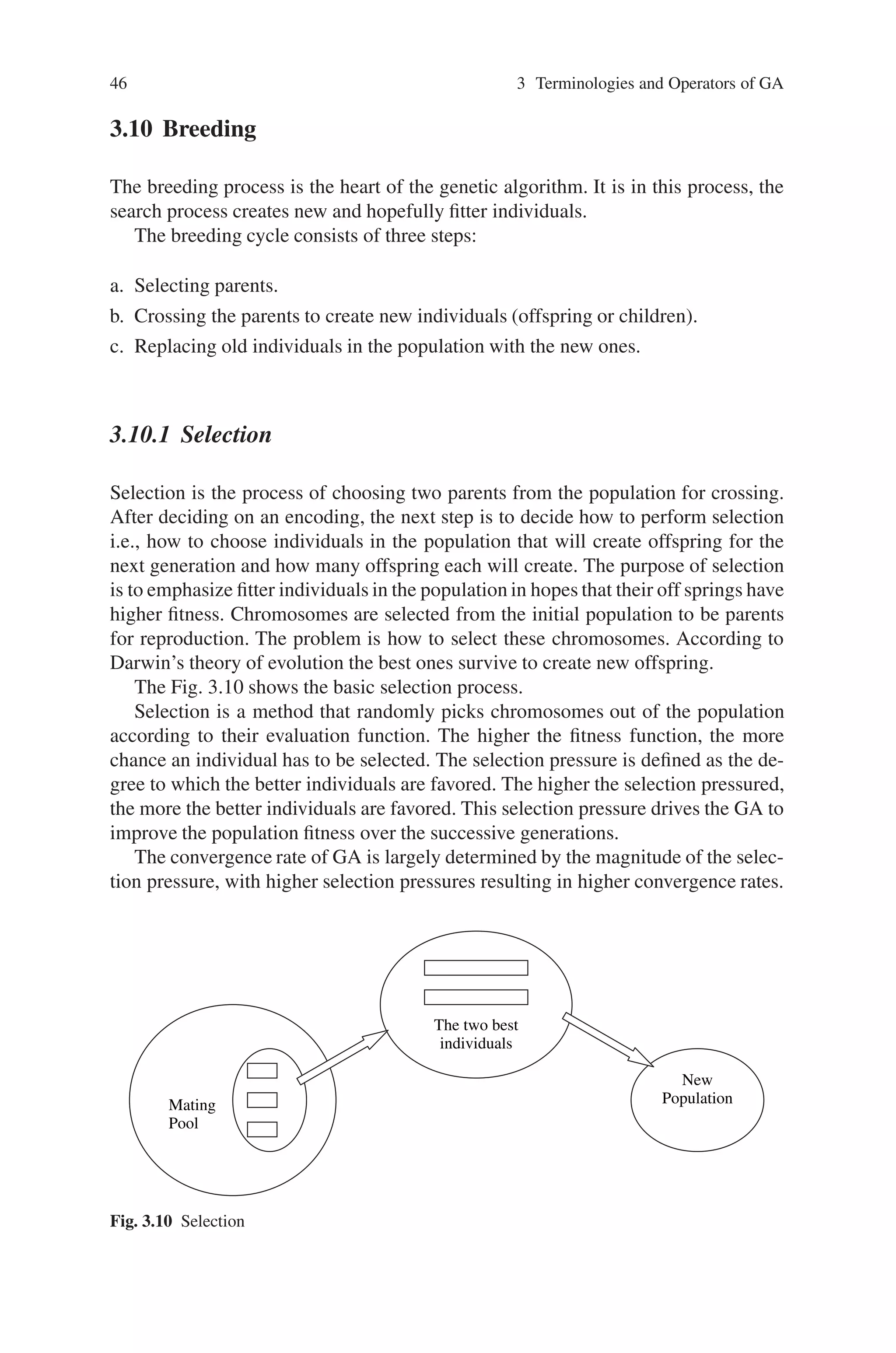
The flowchart showing the process of GA is as shown in Fig. 2.10.
Before implementing GAs it is important to understand few guidelines for de-
signing a general search algorithm i.e. a global optimization algorithm based on
the properties of the fitness landscape and the most common optimization method
types:
1. determinism: A purely deterministic search may have an extremely high variance
in solution quality because it may soon get stuck in worst case situations from
which it is incapable to escape because of its determinism. This can be avoided,
but it is a well-known fact that the observation of the worst-case situation is not
guaranteed to be possible in general.
2. nondeterminism: A stochastic search method usually does not suffer from the
above potential worst case ”wolf trap” phenomenon. It is therefore likely that a
search method should be stochastic, but it may well contain a substantial portion
of determinism, however. In principle it is enough to have as much nondetermin-
ism as to be able to avoid the worst-case wolf traps.
Calculation/
Manipulation
Parents
Decoded String
Reproduction
Mate
Offspring
New
generation
Population
(Chromosomes)
Selection
Evaluation
(Fitness
function)
Generic
Operations
Fig. 2.9 Genetic algorithm cycle](https://image.slidesharecdn.com/s-220425101513/75/S-N-Sivanandam-S-N-Deepa-Introduction-to-Genetic-Algorithms-2008-ISBN-3540731894-pdf-47-2048.jpg)

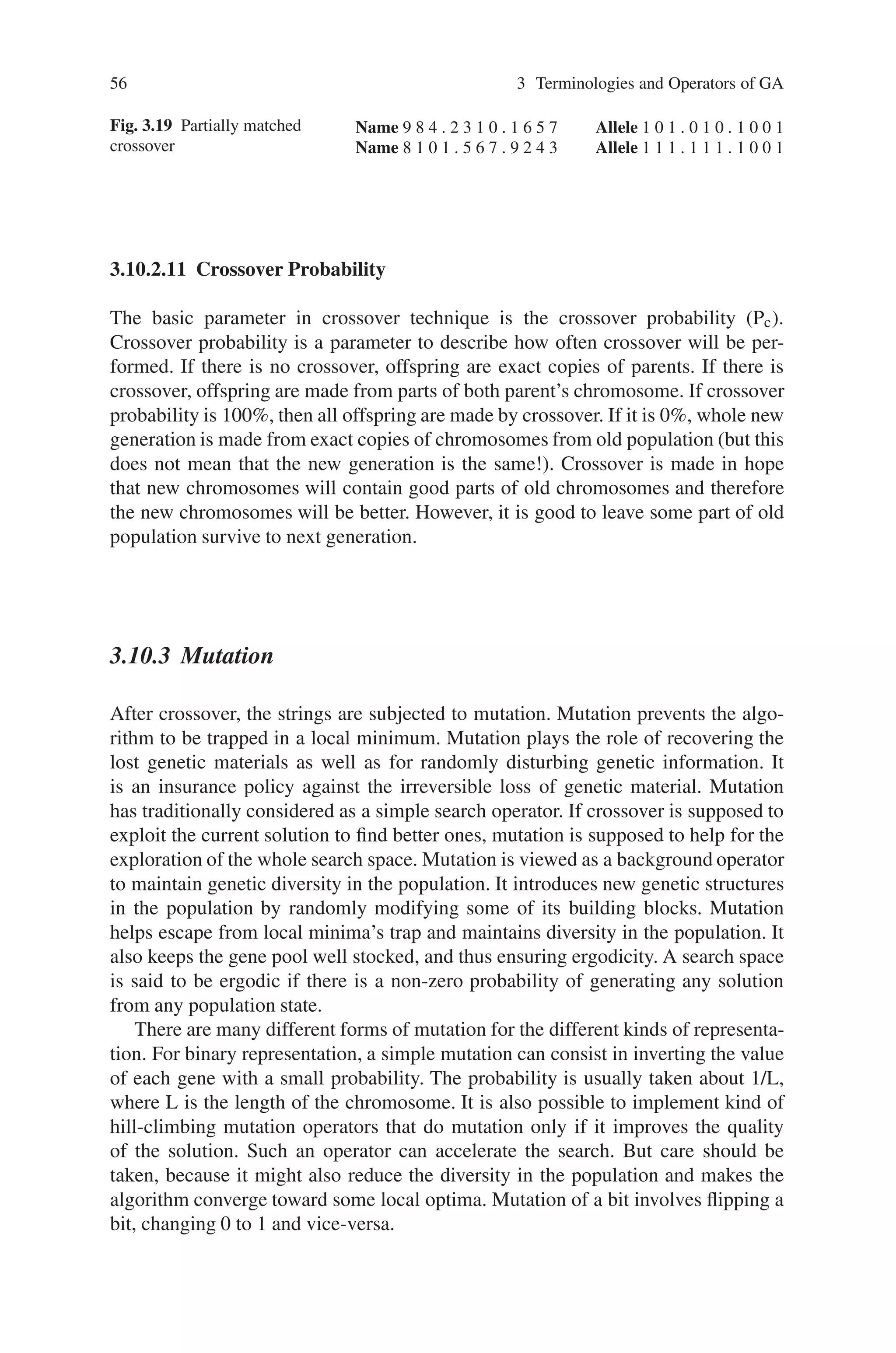
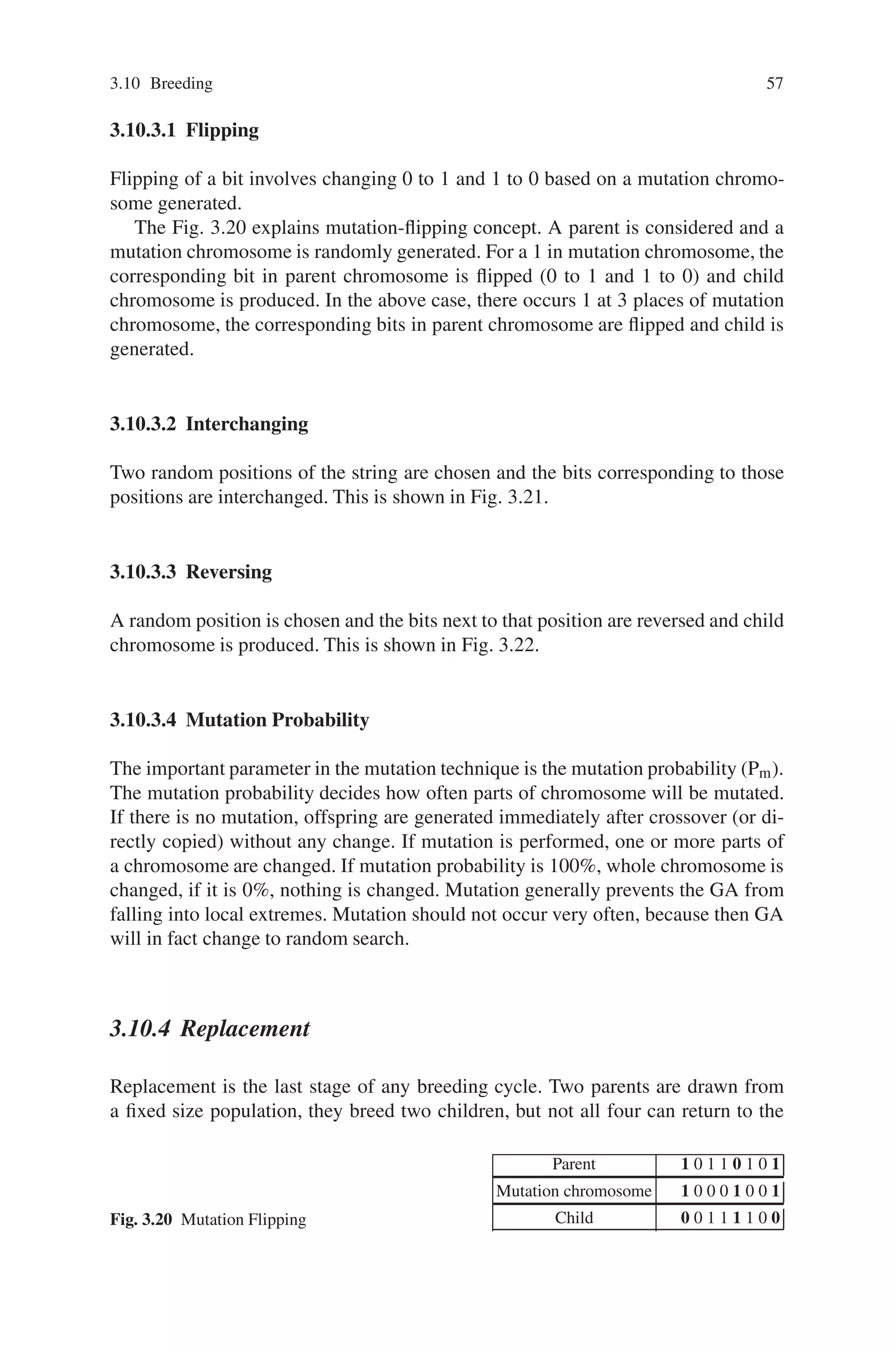
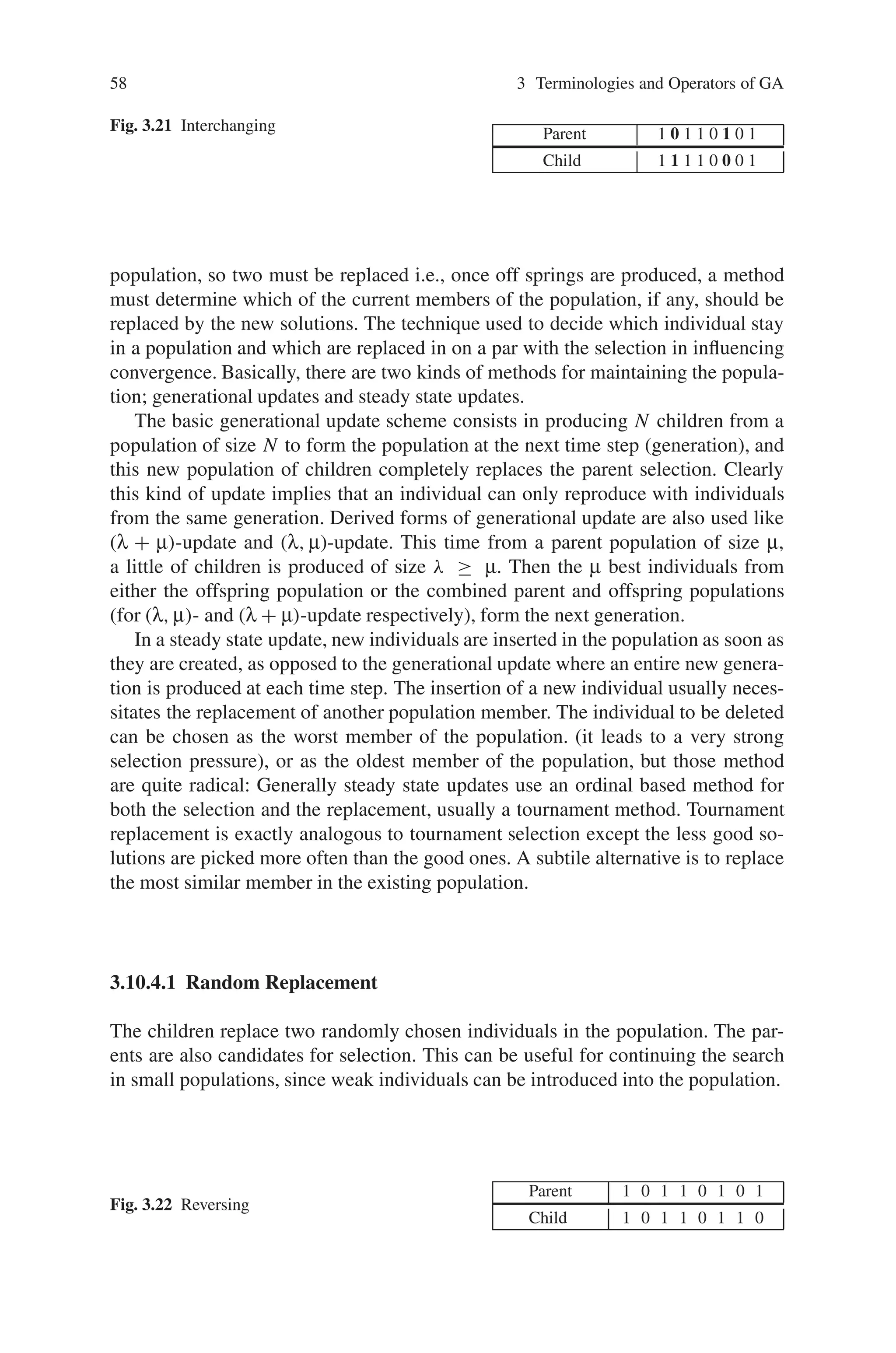
![3.10 Breeding 47
Genetic Algorithms should be able to identify optimal or nearly optimal solutions
under a wise range of selection scheme pressure. However, if the selection pressure
is too low, the convergence rate will be slow, and the GA will take unnecessarily
longer time to find the optimal solution. If the selection pressure is too high, there is
an increased change of the GA prematurely converging to an incorrect (sub-optimal)
solution. In addition to providing selection pressure, selection schemes should also
preserve population diversity, as this helps to avoid premature convergence.
Typically we can distinguish two types of selection scheme, proportionate selec-
tion and ordinal-based selection. Proportionate-based selection picks out individuals
based upon their fitness values relative to the fitness of the other individuals in the
population. Ordinal-based selection schemes selects individuals not upon their raw
fitness, but upon their rank within the population. This requires that the selection
pressure is independent of the fitness distribution of the population, and is solely
based upon the relative ordering (ranking) of the population.
It is also possible to use a scaling function to redistribute the fitness range of the
population in order to adapt the selection pressure. For example, if all the solutions
have their fitness in the range [999, 1000], the probability of selecting a better indi-
vidual than any other using a proportionate-based method will not be important. If
the fitness in every individual is brought to the range [0, 1] equitably, the probability
of selecting good individual instead of bad one will be important.
Selection has to be balanced with variation form crossover and mutation. Too
strong selection means sub optimal highly fit individuals will take over the popula-
tion, reducing the diversity needed for change and progress; too weak selection will
result in too slow evolution. The various selection methods are discussed as follows:
3.10.1.1 Roulette Wheel Selection
Roulette selection is one of the traditional GA selection techniques. The commonly
used reproduction operator is the proportionate reproductive operator where a string
is selected from the mating pool with a probability proportional to the fitness. The
principle of roulette selection is a linear search through a roulette wheel with the
slots in the wheel weighted in proportion to the individual’s fitness values. A target
value is set, which is a random proportion of the sum of the fit nesses in the popula-
tion. The population is stepped through until the target value is reached. This is only
a moderately strong selection technique, since fit individuals are not guaranteed to
be selected for, but somewhat have a greater chance. A fit individual will contribute
more to the target value, but if it does not exceed it, the next chromosome in line
has a chance, and it may be weak. It is essential that the population not be sorted by
fitness, since this would dramatically bias the selection.
The above described Roulette process can also be explained as follows: The ex-
pected value of an individual is that fitness divided by the actual fitness of the popu-
lation. Each individual is assigned a slice of the roulette wheel, the size of the slice
being proportional to the individual’s fitness. The wheel is spun N times, where N is
the number of individuals in the population. On each spin, the individual under the
wheel’s marker is selected to be in the pool of parents for the next generation.](https://image.slidesharecdn.com/s-220425101513/75/S-N-Sivanandam-S-N-Deepa-Introduction-to-Genetic-Algorithms-2008-ISBN-3540731894-pdf-62-2048.jpg)
![3.10 Breeding 49
The best individual from the tournament is the one with the highest fitness, which
is the winner of Nu. Tournament competitions and the winner are then inserted into
the mating pool. The tournament competition is repeated until the mating pool for
generating new offspring is filled. The mating pool comprising of the tournament
winner has higher average population fitness. The fitness difference provides the
selection pressure, which drives GA to improve the fitness of the succeeding genes.
This method is more efficient and leads to an optimal solution.
3.10.1.5 Boltzmann Selection
Simulation annealing is a method of function minimization or maximization. This
method simulates the process of slow cooling of molten metal to achieve the mini-
mum function value in a minimization problem. Controlling a temperature like pa-
rameter introduced with the concept of Boltzmann probability distribution simulates
the cooling phenomenon.
In Boltzmann selection a continuously varying temperature controls the rate of
selection according to a preset schedule. The temperature starts out high, which
means the selection pressure is low. The temperature is gradually lowered, which
gradually increases the selection pressure, thereby allowing the GA to narrow in
more closely to the best part of the search space while maintaining the appropriate
degree of diversity.
A logarithmically decreasing temperature is found useful for convergence with-
out getting stuck to a local minima state. But to cool down the system to the equi-
librium state takes time.
Let fmax be the fitness of the currently available best string. If the next string has
fitness f(Xi ) such that f(Xi)fmax, then the new string is selected. Otherwise it is
selected with Boltz Mann probability,
P = exp[−(fmax-f(Xi))/T] (3.1)
Where T = To(1-α)k and k = (1 + 100∗g/G); g is the current generation number;
G, the maximum value of g. The value of α can be chosen from the range [0, 1] and
To from the range [5, 100]. The final state is reached when computation approaches
zero value of T, i.e., the global solution is achieved at this point.
The probability that the best string is selected and introduced into the mating
pool is very high. However, Elitism can be used to eliminate the chance of any
undesired loss of information during the mutation stage. Moreover, the execution
time is less.
Elitism
The first best chromosome or the few best chromosomes are copied to the new popu-
lation. The rest is done in a classical way. Such individuals can be lost if they are not
selected to reproduce or if crossover or mutation destroys them. This significantly
improves the GA’s performance.](https://image.slidesharecdn.com/s-220425101513/75/S-N-Sivanandam-S-N-Deepa-Introduction-to-Genetic-Algorithms-2008-ISBN-3540731894-pdf-64-2048.jpg)
![50 3 Terminologies and Operators of GA
3.10.1.6 Stochastic Universal Sampling
Stochastic universal sampling provides zero bias and minimum spread. The indi-
viduals are mapped to contiguous segments of a line, such that each individual’s
segment is equal in size to its fitness exactly as in roulette-wheel selection. Here
equally spaced pointers are placed over the line, as many as there are individuals to
be selected. Consider NPointer the number of individuals to be selected, then the
distance between the pointers are 1/NPointer and the position of the first pointer is
given by a randomly generated number in the range [0, 1/NPointer].
For 6 individuals to be selected, the distance between the pointers is 1/6 = 0.167.
Figure 3.11 shows the selection for the above example.
Sample of 1 random number in the range [0, 0.167]: 0.1.
After selection the mating population consists of the individuals,
1, 2, 3, 4, 6, 8.
Stochastic universal sampling ensures a selection of offspring, which is closer to
what is deserved than roulette wheel selection.
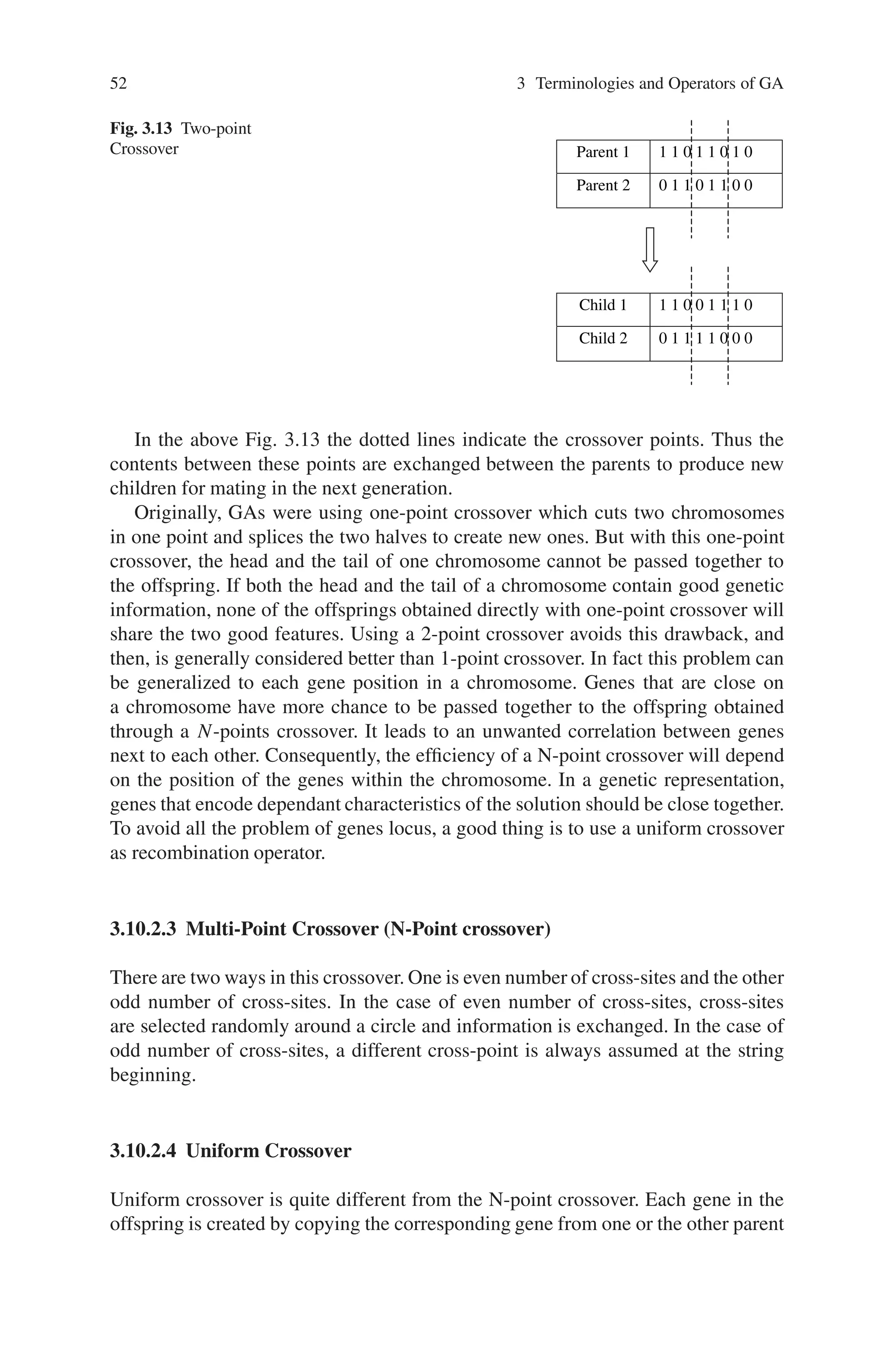
3.10.2 Crossover (Recombination)
Crossover is the process of taking two parent solutions and producing from them
a child. After the selection (reproduction) process, the population is enriched with
better individuals. Reproduction makes clones of good strings but does not create
new ones. Crossover operator is applied to the mating pool with the hope that it
creates a better offspring.
Crossover is a recombination operator that proceeds in three steps:
i. The reproduction operator selects at random a pair of two individual strings for
the mating.
ii. A cross site is selected at random along the string length.
iii. Finally, the position values are swapped between the two strings following the
cross site.
Fig. 3.11 Stochastic universal sampling](https://image.slidesharecdn.com/s-220425101513/75/S-N-Sivanandam-S-N-Deepa-Introduction-to-Genetic-Algorithms-2008-ISBN-3540731894-pdf-65-2048.jpg)
![64 3 Terminologies and Operators of GA
chromosomes, the Gas process O(n3) schemata into each generation. This is called
as implicit parallel process.
A schema represents an affined variety of the search space: for example the
schema 01**11*0 is a sub-space of the space of codes of 8 bits length (∗ can be
0 or 1).
The GA modeled in schema theory is a canonical GA, which acts on binary
strings, and for which the creation of a new generation is based on three operators:
– A proportionate selection, where the fitness function steps in: the probability that
a solution of the current population is selected and is proportional to its fitness.
– The genetic operators: single point crossover and bit-flip mutation, randomly ap-
plied with probabilities pc and pm.
Schemata represent global information about the fitness function. A GA works
on a population of N codes, and implicitly uses information on a certain number of
schemata. The basic ‘schema theorem’ presented below is based on the observation
that the evaluation of a single code makes it possible to deduce some knowledge
about the schemata to which that code belongs.
Theorem :( Schema Theorem (Holland))
The Schema Theorem is called as “The Fundamental Theorem of Genetic
Algorithm”.
For a given schema H, let:
– m (H, t) be the relative frequency of the schema H in the population of the tth
generation.
– f(H) be the mean fitness of the elements of H.
– O(H) be the number of fixed bits in the schema H, called the order of the schema.
– δ(H) be distance between the first and the last fixed bit of the schema, called the
definition length of the schema.
– f̄ is the mean fitness of the current population.
– Pc is the crossover probability.
– Pm is the mutation probability.
Then,
E [m(H, t + 1)] ≥ m(H, t)
f(H)
f̄
1 − Pc
δ(H)
1-1
− O(H)Pm
(3.2)
Based on qualitative view, the above formula means that the “good” schemata,
having a short definition length and a low order, tend to grow very rapidly in the
population. These particular schemata are called building blocks.
The application of schema theorem is as follows:
i. It provides some tools to check whether a given representation is well-suited
to a GA.](https://image.slidesharecdn.com/s-220425101513/75/S-N-Sivanandam-S-N-Deepa-Introduction-to-Genetic-Algorithms-2008-ISBN-3540731894-pdf-79-2048.jpg)
![4.3 Multiploid 85
Diploid chromosomes lend advantages to individuals where the environment may
change over a period of time. Having two genes allows two different solutions to be
remembered, and passed on to offspring. One of these will be dominant (i.e., it will
be expressed in the phenotype), while the other will be recessive. If environmental
conditions change, the dominance can shift, so that the other gene is dominant. This
shift can take place much more quickly than would be possible if evolutionary mech-
anisms had to alter the gene. This mechanism is ideal if the environment regularly
switches between two states (e.g., ice-age, non ice-age). The primary advantage
of diploidy is that it allows a wider diversity of alleles to be kept in the population,
compared with haploidy. Currently harmful, but potentially useful alleles can still be
maintained, but in a recessive position. Other genetic mechanisms could achieve the
same effect. For example, a chromosome might contain several variants of a gene.
Epistasis (in the sense of masking) could be used to ensure that only one of the
variants was expressed in any particular individual. A situation like this occurs with
haemoglobin production. Different genes code for its production during different
stages of development. During the foetal stage, one gene is switched on to produce
haemoglobin, whilst later on a different gene is activated. There are a variety of
biological metaphors we can use to inspire our development of GAs.
In a GA, diploidy might be useful in an on-line application where the system
could switch between different states. Diploidy involves a significant overhead in a
GA. As well as carrying twice as much genetic information, the chromosome must
also carry dominance information.
4.3 Multiploid
A multiploid genetic algorithm incorporates several candidates for each gene within
a single genotype, and uses some form of dominance mechanism to decide which
choice of each gene is active in the phenotype. In nature we find that many organ-
isms have poly-ploid genotypes, which consist of multiple sets of chromosomes
with some mechanism for determining which gene is expressed i.e., is dominant at
each locus. This mechanism seems to confer a number of advantages on a system,
mainly by enhancing population diversity; currently unused genes remains in a mul-
tiplied genotype, unexpressed, but shielded from extinction until they may become
useful later.
A multiploid genotype, shown in Fig. 4.2, contains p chromosomes, each of
length L, and a mask which specifies which of the p chromosomes has the dominant
gene at a particular position in the chromosome. This information is decoded to
yield the phenotype as follows:
Fig. 4.2 Multiploid Type 1
Mask 0 0 0 1 1 1 2 2 2
Chromosome [0]: a a a a A a a a a
Chromosome [1]: b b b b B b b b b
Chromosome [2]: c c c c C c c c c
Phenotype: a a a b B b c c c](https://image.slidesharecdn.com/s-220425101513/75/S-N-Sivanandam-S-N-Deepa-Introduction-to-Genetic-Algorithms-2008-ISBN-3540731894-pdf-99-2048.jpg)
![86 4 Advanced Operators and Techniques in Genetic Algorithm
Fig. 4.3 Multiploid Type 2 Mask 0 1 2
Chromosome [0]: a a a a a a a a a
Chromosome [1]: b b b b b b b b b
Chromosome [2]: c c c c c c c c c
Phenotype: a a a b b b c c c
An allele value of a at locus i in the mask denotes that the ith gene in the chro-
mosome with index a becomes the ith gene of the phenotype. The mask length can
be shorter than the length of the chromosomes, as in Fig. 4.3.
In Fig. 4.3, if the mask length is m and the chromosome length L, then a gene at
locus ‘i’ in the mask with the value of ‘a’ indicates that the i-th set of L/m consecu-
tives genes in the a-th chromosome are dominant.
4.4 Inversion and Reordering
Inversion is a unary, reordering genetic operator. Simple genetic algorithms use
stochastic selection, 1-point cross over, and mutation to increase the number of
building blocks in the population and to recombine them for even better build-
ing blocks. The building blocks being highly fit, low order, short defining length
schemes, the encoding scheme chosen must be compatible with this. Can we search
for better encoding schemes while searching for building blocks? To answer this
question, inversion operator was created.
Inversion operator is a primary natural mechanism to recode a problem. In in-
version operator, two points are selected along the length of the chromosome, the
chromosome is cut at those points and the end points of the section cut, gets re-
versed (switched, swapped). To make it clear, consider a chromosome of length 8
where two inverse points are selected random (the points are 2 and 6 denoted byˆ
character):
1 1 ∧ 0 1 1 1 ∧ 0 1
On using inversion operator, the string becomes,
1 1 1 1 1 0 0 1
Thus within the specified inversion points, the switching between the chromo-
somes takes place.
The inversion operator can also be used for extended representation as given by,
1 2 3 4 5 6 7 8
1 1 ∧ 0 1 1 1 ∧ 0 1
Inversion points are chosen at random (indicated by operator) and the chromo-
some now becomes,](https://image.slidesharecdn.com/s-220425101513/75/S-N-Sivanandam-S-N-Deepa-Introduction-to-Genetic-Algorithms-2008-ISBN-3540731894-pdf-100-2048.jpg)

![= i1 between 0 and ; inclusive;
if i1 i2 then
swap i1 and i2;
end
for I=i1 to [(i1+i2-1)/2] do
swap allele and index at locus I with allele and index at locus.
i1+i2-1-I;
end
Thus an index is needed for each locus to preserve the meaning of the locus inde-
pendent of its position on the chromosome. Inversion is redundant with operators
such as UX (Uniform Crossover), which do not have any positional bias.
There are several other reordering operators, which being variations on inversion.
They are:
1. Linear inversion.
2. Liner + end inversion.
3. Continuous inversion.
4. Mass inversion.
Linear inversion is the inversion, which has been discussed earlier. Linear + end
inversion is a linear inversion with a specified probability of (0.75). When linear
inversion is not performed, end inversion would be done with equal probability](https://image.slidesharecdn.com/s-220425101513/75/S-N-Sivanandam-S-N-Deepa-Introduction-to-Genetic-Algorithms-2008-ISBN-3540731894-pdf-102-2048.jpg)
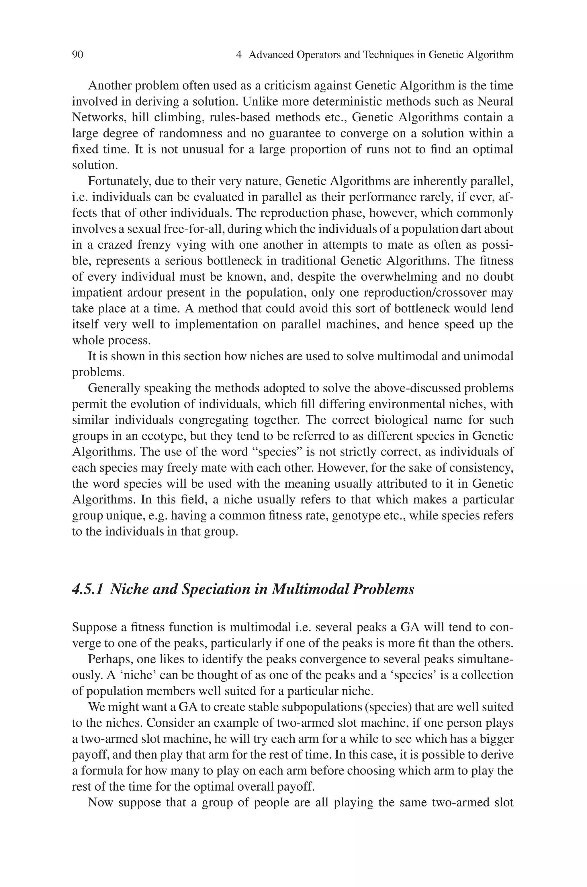
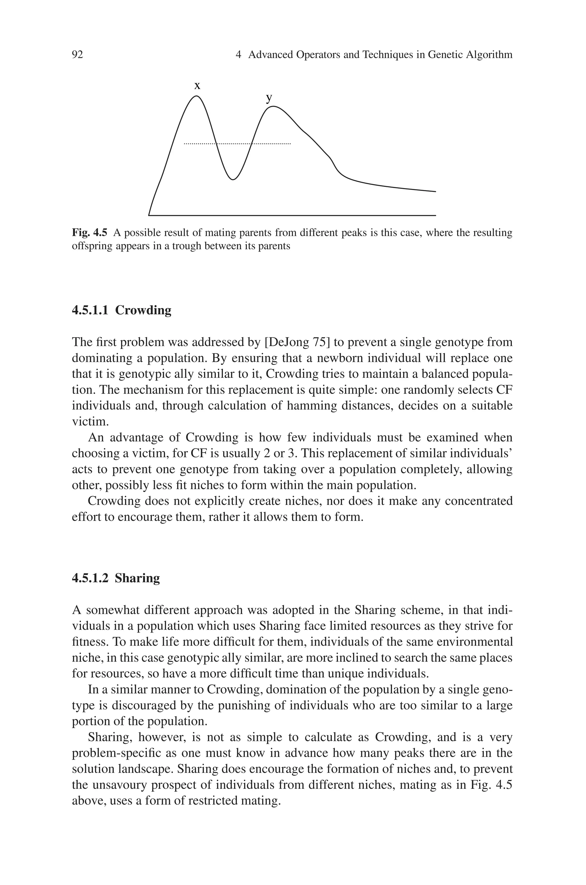
![92 4 Advanced Operators and Techniques in Genetic Algorithm
x
y
Fig. 4.5 A possible result of mating parents from different peaks is this case, where the resulting
offspring appears in a trough between its parents
4.5.1.1 Crowding
The first problem was addressed by [DeJong 75] to prevent a single genotype from
dominating a population. By ensuring that a newborn individual will replace one
that it is genotypic ally similar to it, Crowding tries to maintain a balanced popula-
tion. The mechanism for this replacement is quite simple: one randomly selects CF
individuals and, through calculation of hamming distances, decides on a suitable
victim.
An advantage of Crowding is how few individuals must be examined when
choosing a victim, for CF is usually 2 or 3. This replacement of similar individuals’
acts to prevent one genotype from taking over a population completely, allowing
other, possibly less fit niches to form within the main population.
Crowding does not explicitly create niches, nor does it make any concentrated
effort to encourage them, rather it allows them to form.
4.5.1.2 Sharing
A somewhat different approach was adopted in the Sharing scheme, in that indi-
viduals in a population which uses Sharing face limited resources as they strive for
fitness. To make life more difficult for them, individuals of the same environmental
niche, in this case genotypic ally similar, are more inclined to search the same places
for resources, so have a more difficult time than unique individuals.
In a similar manner to Crowding, domination of the population by a single geno-
type is discouraged by the punishing of individuals who are too similar to a large
portion of the population.
Sharing, however, is not as simple to calculate as Crowding, and is a very
problem-specific as one must know in advance how many peaks there are in the
solution landscape. Sharing does encourage the formation of niches and, to prevent
the unsavoury prospect of individuals from different niches, mating as in Fig. 4.5
above, uses a form of restricted mating.](https://image.slidesharecdn.com/s-220425101513/75/S-N-Sivanandam-S-N-Deepa-Introduction-to-Genetic-Algorithms-2008-ISBN-3540731894-pdf-107-2048.jpg)


![6.8 Haploid Genetic Programming with Dominance 159
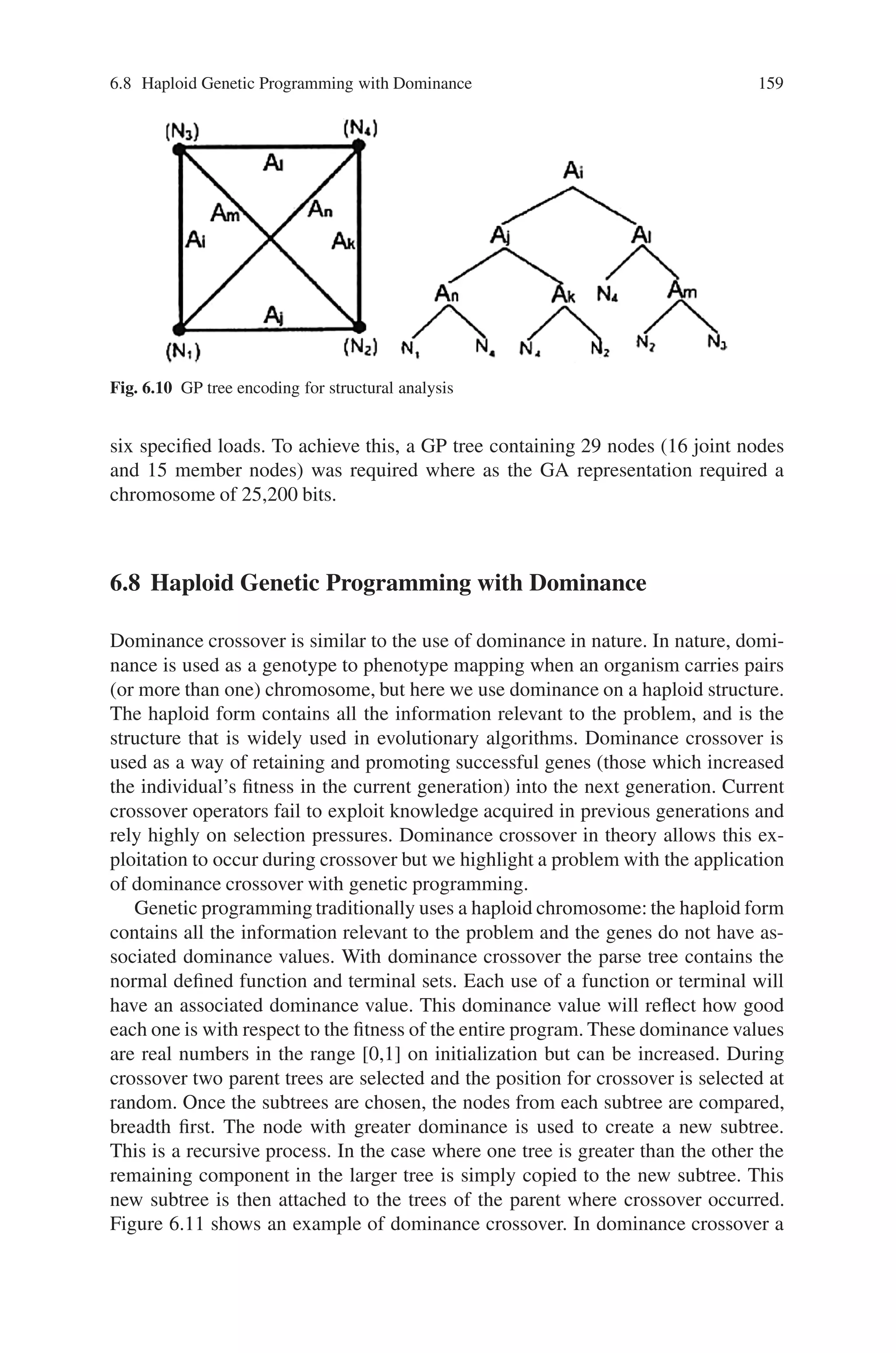
Fig. 6.10 GP tree encoding for structural analysis
six specified loads. To achieve this, a GP tree containing 29 nodes (16 joint nodes
and 15 member nodes) was required where as the GA representation required a
chromosome of 25,200 bits.
6.8 Haploid Genetic Programming with Dominance
Dominance crossover is similar to the use of dominance in nature. In nature, domi-
nance is used as a genotype to phenotype mapping when an organism carries pairs
(or more than one) chromosome, but here we use dominance on a haploid structure.
The haploid form contains all the information relevant to the problem, and is the
structure that is widely used in evolutionary algorithms. Dominance crossover is
used as a way of retaining and promoting successful genes (those which increased
the individual’s fitness in the current generation) into the next generation. Current
crossover operators fail to exploit knowledge acquired in previous generations and
rely highly on selection pressures. Dominance crossover in theory allows this ex-
ploitation to occur during crossover but we highlight a problem with the application
of dominance crossover with genetic programming.
Genetic programming traditionally uses a haploid chromosome: the haploid form
contains all the information relevant to the problem and the genes do not have as-
sociated dominance values. With dominance crossover the parse tree contains the
normal defined function and terminal sets. Each use of a function or terminal will
have an associated dominance value. This dominance value will reflect how good
each one is with respect to the fitness of the entire program. These dominance values
are real numbers in the range [0,1] on initialization but can be increased. During
crossover two parent trees are selected and the position for crossover is selected at
random. Once the subtrees are chosen, the nodes from each subtree are compared,
breadth first. The node with greater dominance is used to create a new subtree.
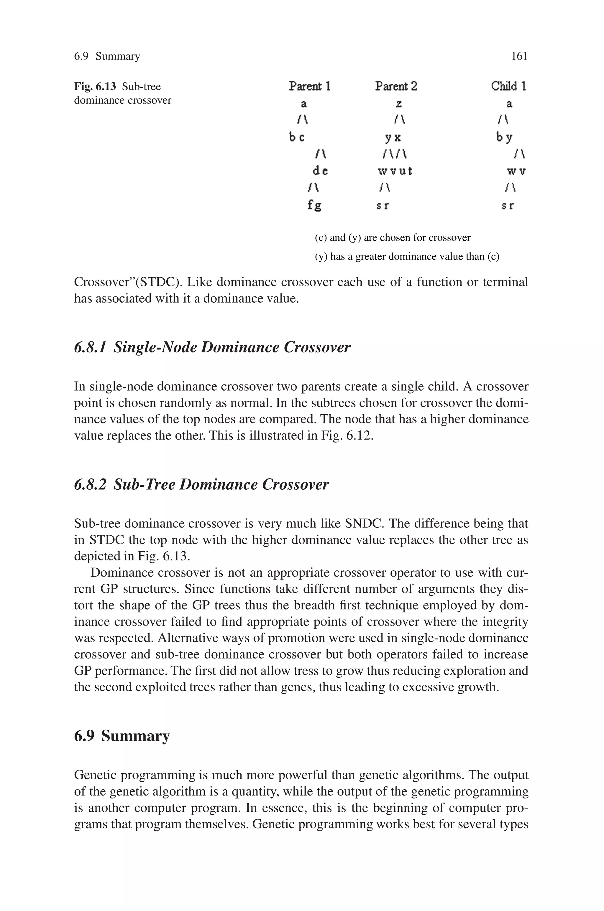
This is a recursive process. In the case where one tree is greater than the other the
remaining component in the larger tree is simply copied to the new subtree. This
new subtree is then attached to the trees of the parent where crossover occurred.
Figure 6.11 shows an example of dominance crossover. In dominance crossover a](https://image.slidesharecdn.com/s-220425101513/75/S-N-Sivanandam-S-N-Deepa-Introduction-to-Genetic-Algorithms-2008-ISBN-3540731894-pdf-173-2048.jpg)
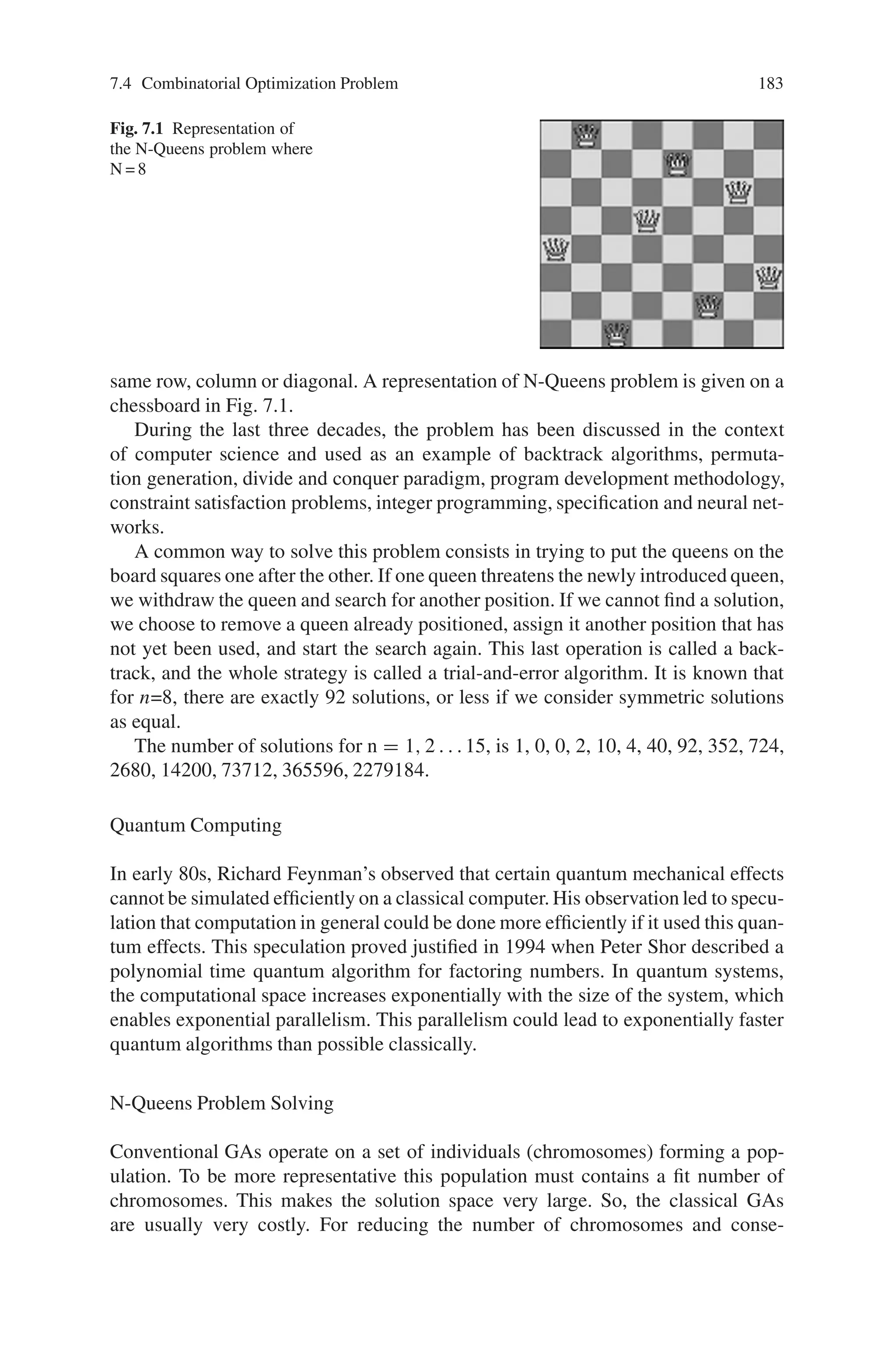
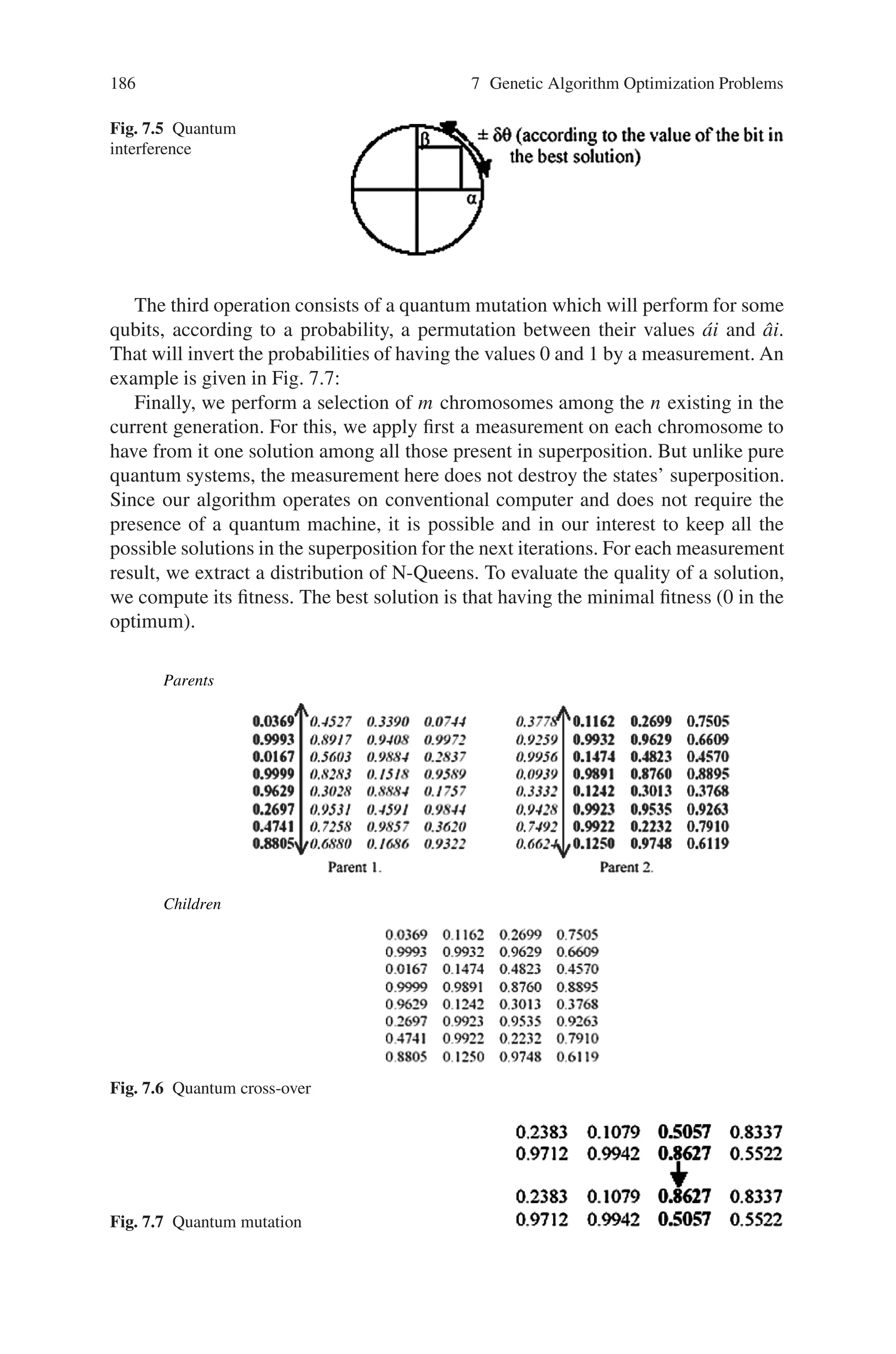
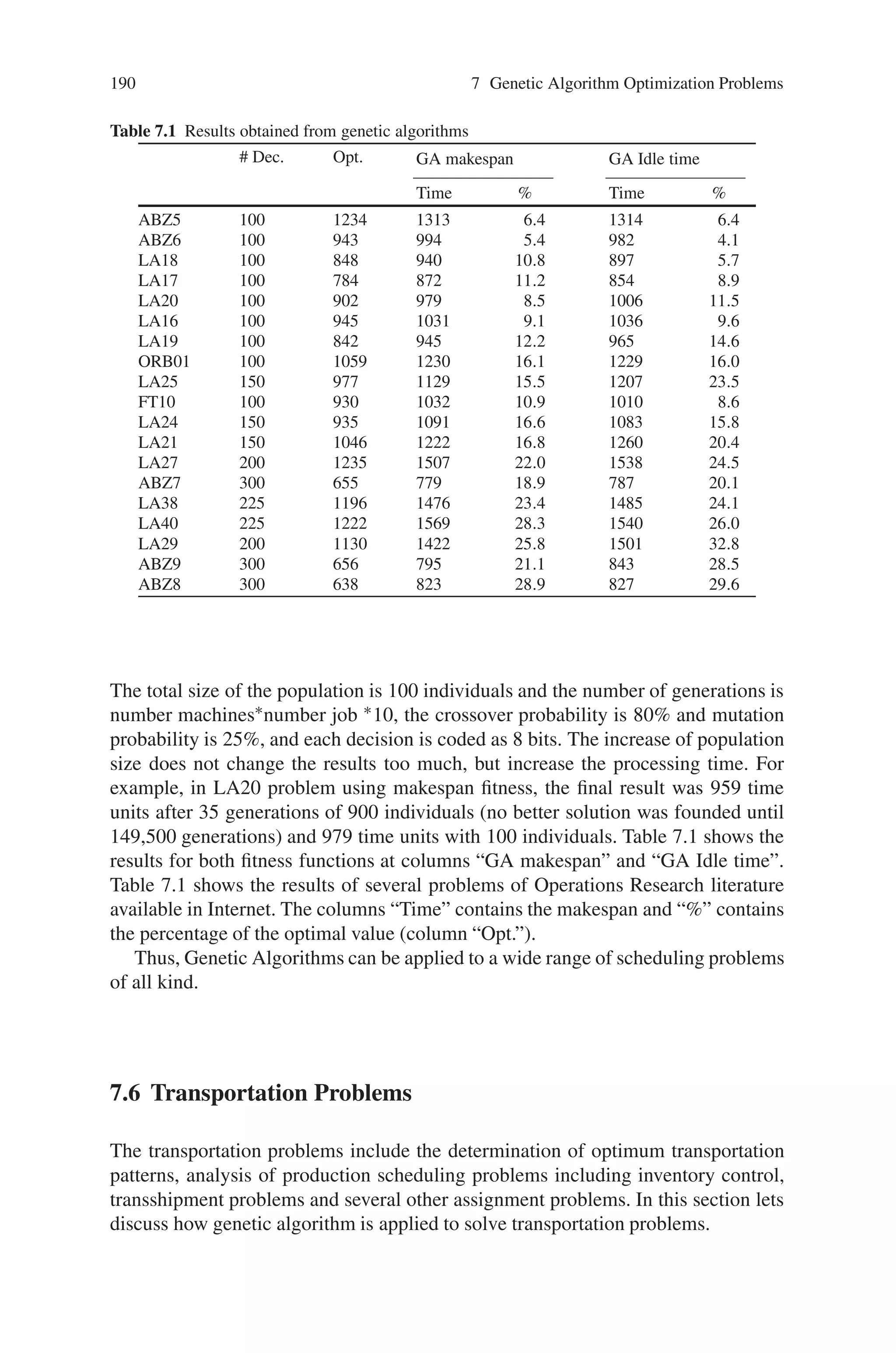
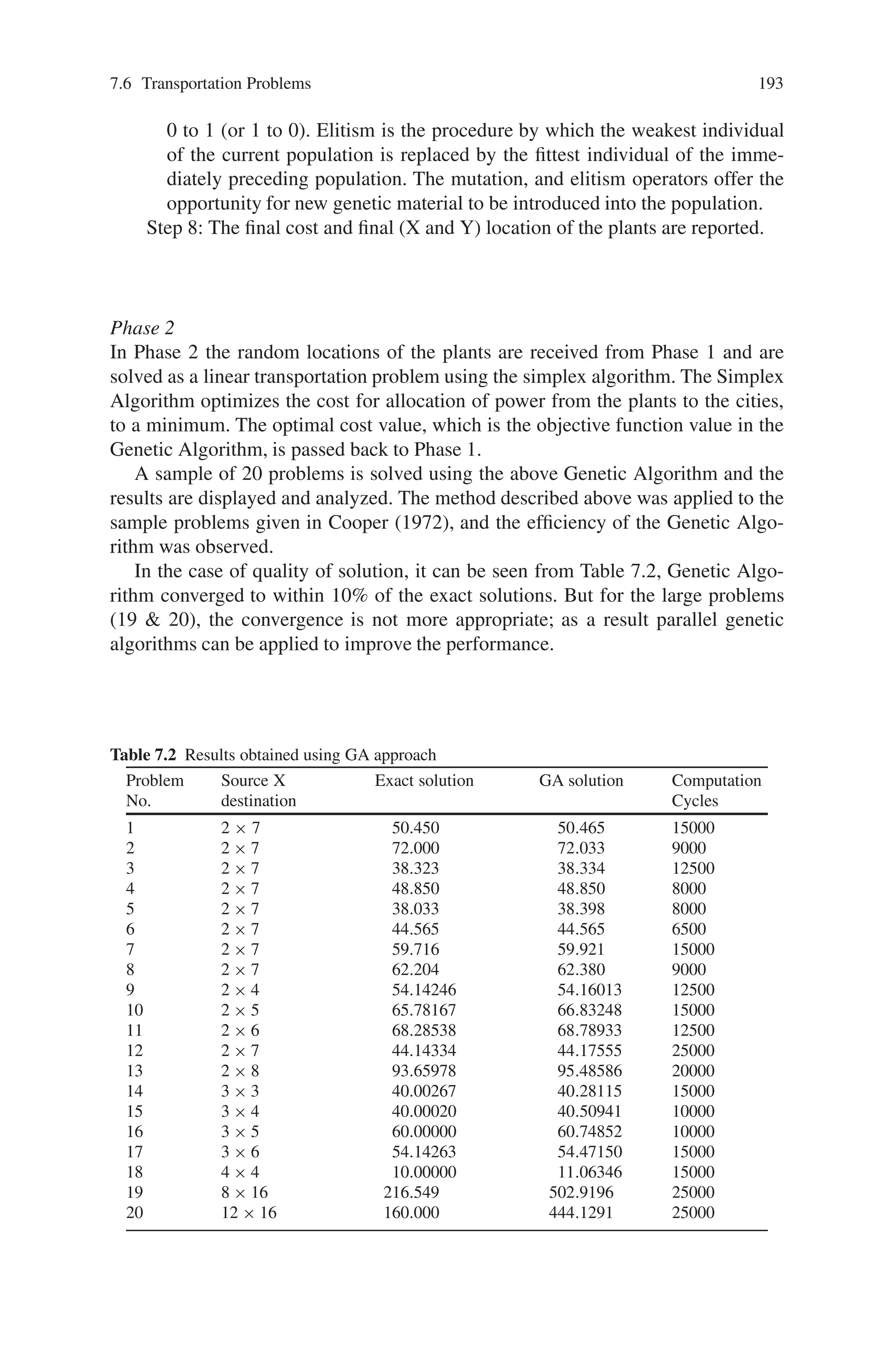
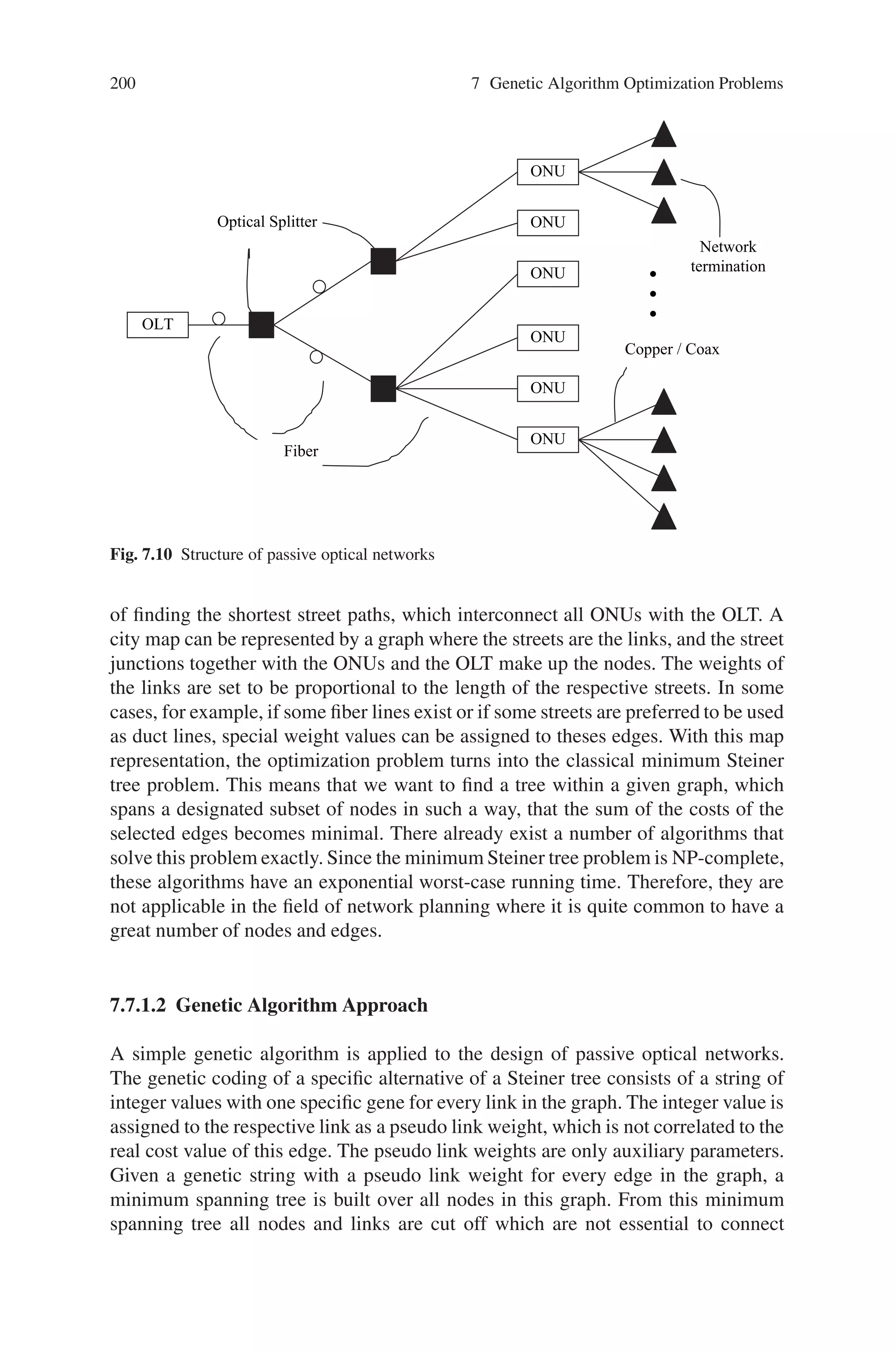
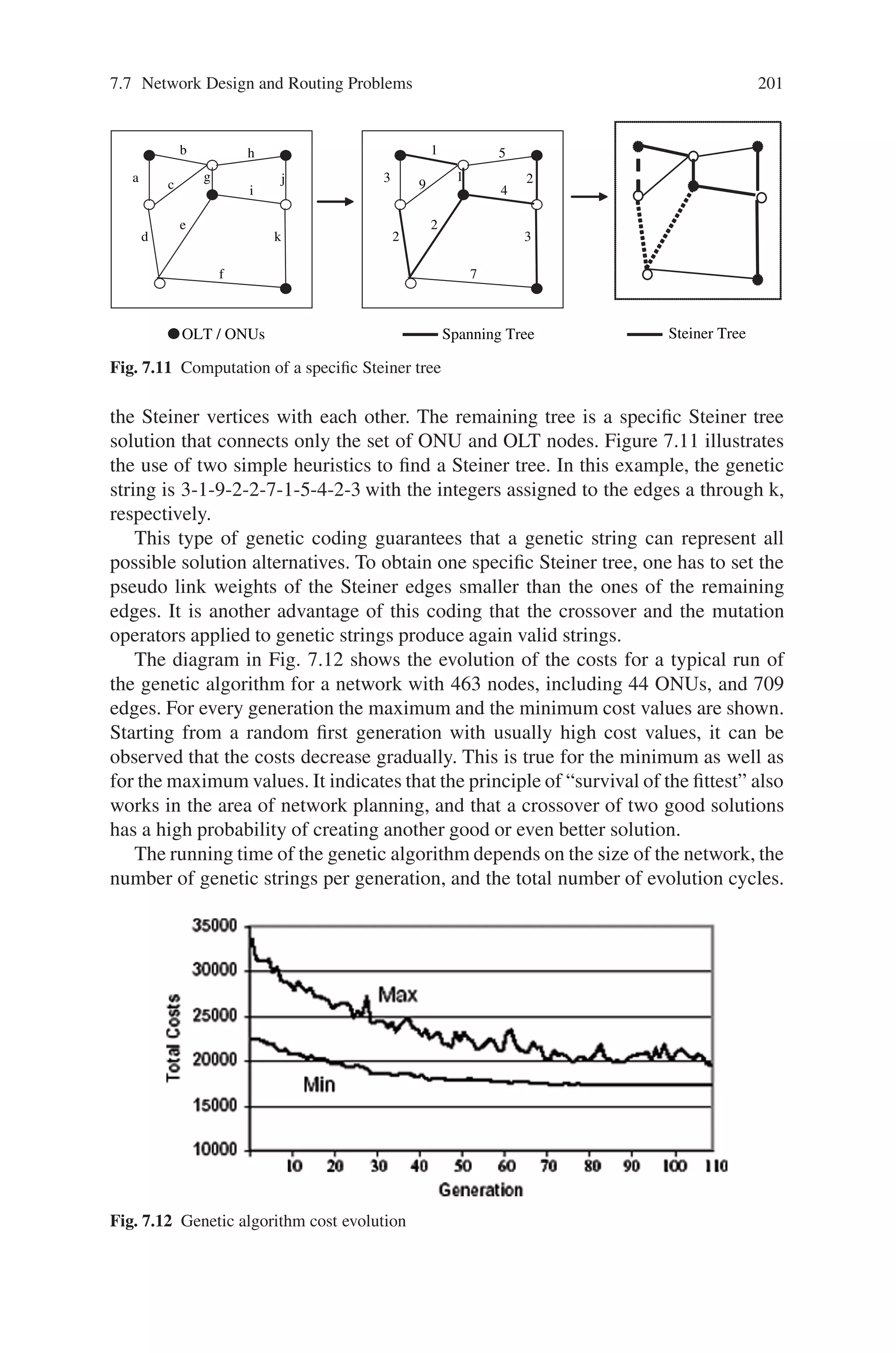
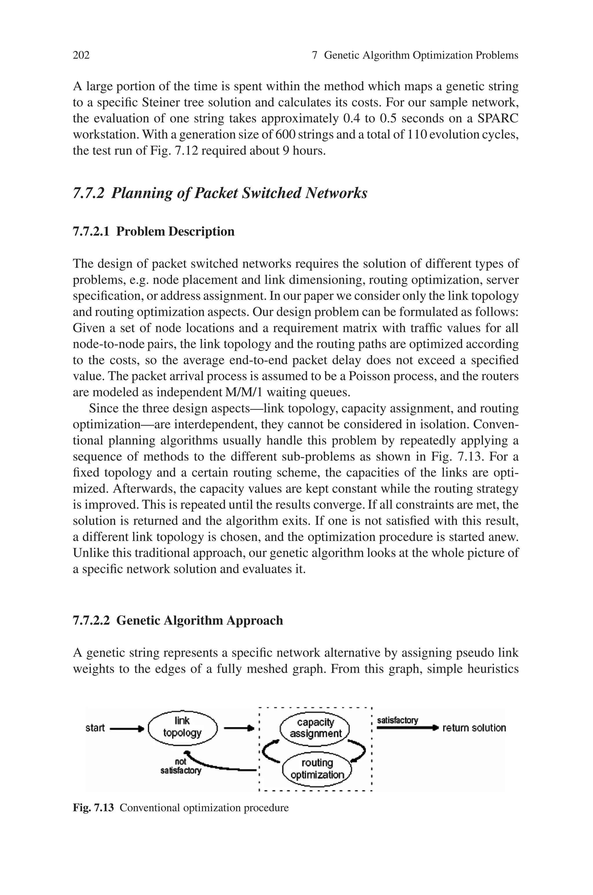
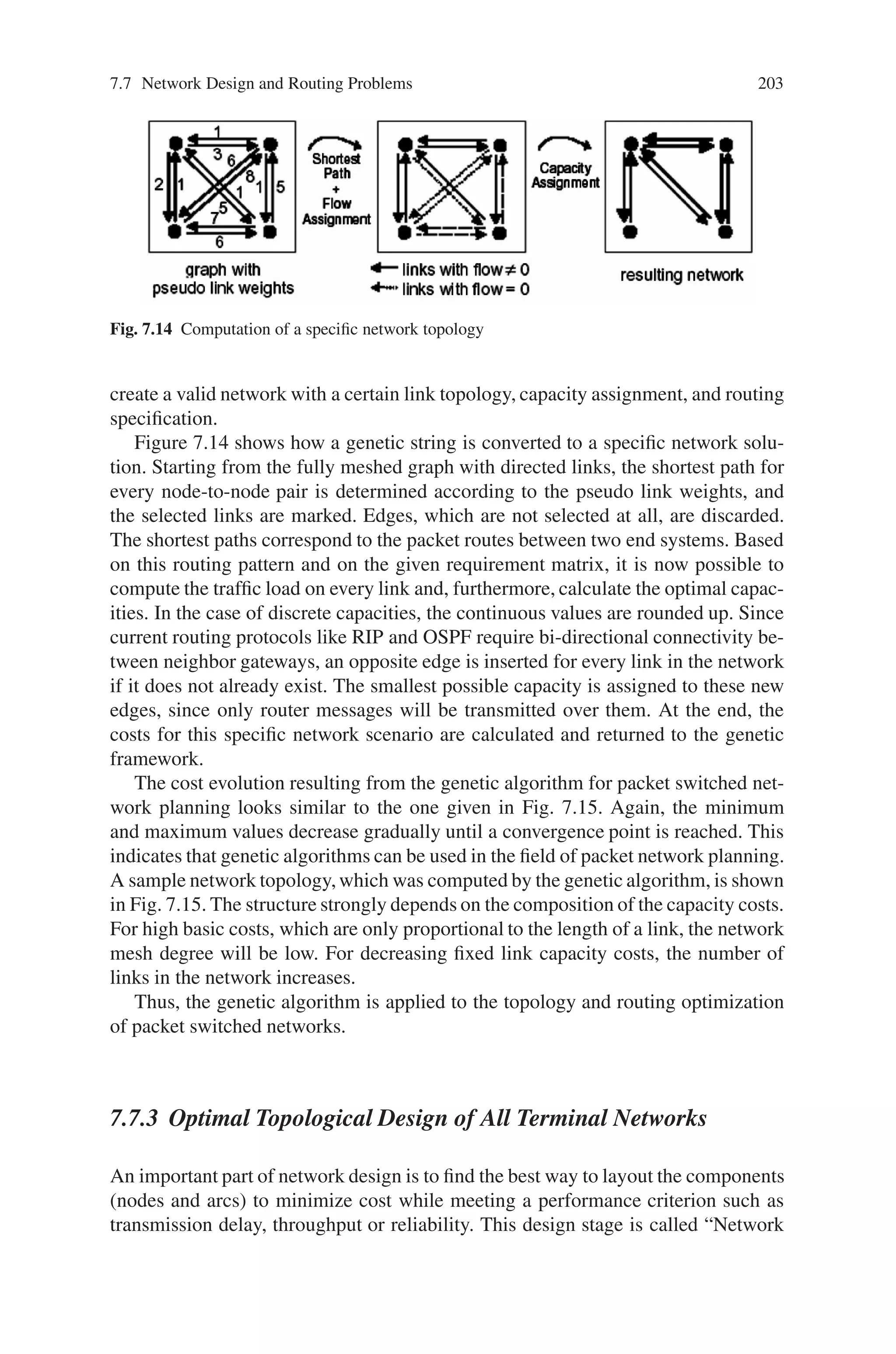
![172 7 Genetic Algorithm Optimization Problems
At a particular time, only few edges of G might be operational. An operational
state of G is a sub-graph G’ = (V, E’). The network reliability of state E’ ⊆ E is as
follows:
#
e∈E
pe
$ ⎛
⎝
#
e∈E|E
qe
⎞
⎠ (7.8)
7.3.1.2 Genetic Algorithm Approach
This section proposes a genetic algorithm for the design of networks when consider-
ing all terminal reliability. The assumption made here is that reliability of all edges in
the network are identical, whereas cost depends on which two nodes are connected.
It should be noted that only one reliability and cost alternative is available for each
pair of nodes. This approach allows edges to be chosen from different components
with different costs and reliabilities. The following notations are used to describe
the optimal design of the network, allowing edges to be chosen from different edge
options:
k is the number of options for the edge connection
t is the option between nodes
xij is an edge option for the edge between nodes i and j
p(xij) is the reliability design option and
c(xij) is a unit cost of the edge option
Representation: As each network design x is easily formed into an integer vector,
it can be used as a chromosome for the genetic algorithm. Each element of the
chromosome represents a possible edge in the network design problem, so there
are n × (n−1)/2 vector components in each candidate architecture x. The value of
each element tells what type of connection the specific edge has with the pair of
nodes it connects. The only possible values allowed in each position of the chro-
mosome are 0, 1, . . . , k−1. The solution space of possible network architectures is
k(n×(n−1))/2.
Fitness: The fitness function is to find the minimum-cost network architecture
that meets or exceeds prespecified network reliability, Rmin. Construction of fitness
function is that it may consider infeasible network architectures, because infea-
sible solutions may contain beneficial information. Also, breeding two infeasible
solutions or an infeasible solution with a feasible solution can yield a good fea-
sible solution. The optimal design will lie on the boundary between feasible and
infeasible designs, since only one constraint will be active or nearly active for a
minimum cost network. Thus the fitness function for this problem is defined as
follows:
Z p(x) = Z(x) + Z(x∗
)[1 + Rmin − R(x)]rp+(popsize∗ gen)/50
(7.9)](https://image.slidesharecdn.com/s-220425101513/75/S-N-Sivanandam-S-N-Deepa-Introduction-to-Genetic-Algorithms-2008-ISBN-3540731894-pdf-185-2048.jpg)
![7.3 Multiobjective Reliability Design Problem 175
max f1(m, x) =
n
%
i=1
[1 − (1 − xi)mi]
min f2(m, x) =
n
i=1
C(xi)
mi + exp
mi
4
'
such that G1(m) =
n
i=1
wimiexp
mi
4
'
≤ Ws
G2(m) =
n
i=1
vi (mi)2 ≤ Vs
1 ≤ mi ≤ 10, 0.5 ≤ xi ≤ 1 − 10−6 i = 1, . . . , 4
(7.10)
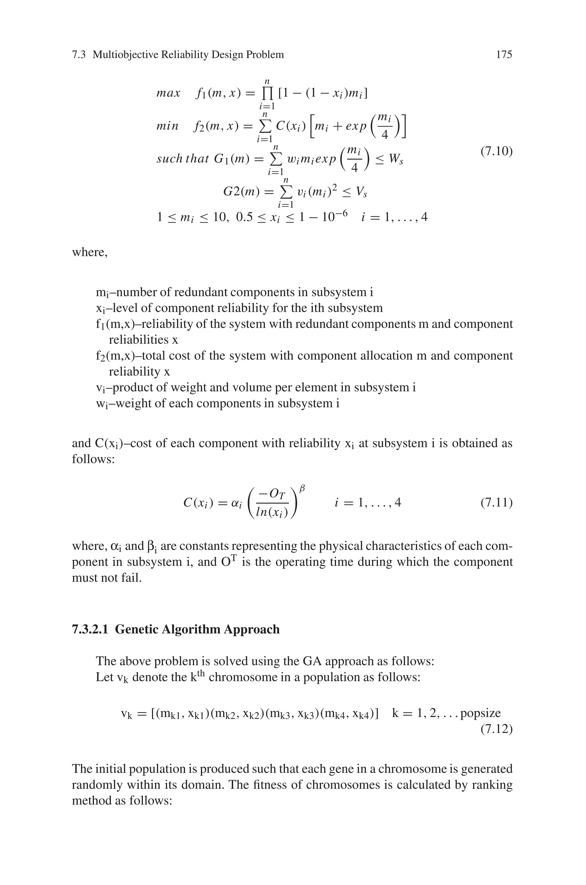
where,
mi–number of redundant components in subsystem i
xi–level of component reliability for the ith subsystem
f1(m,x)–reliability of the system with redundant components m and component
reliabilities x
f2(m,x)–total cost of the system with component allocation m and component
reliability x
vi–product of weight and volume per element in subsystem i
wi–weight of each components in subsystem i
and C(xi)–cost of each component with reliability xi at subsystem i is obtained as
follows:
C(xi ) = αi
−OT
ln(xi)
β
i = 1, . . . , 4 (7.11)
where, αi and βi are constants representing the physical characteristics of each com-
ponent in subsystem i, and OT is the operating time during which the component
must not fail.
7.3.2.1 Genetic Algorithm Approach
The above problem is solved using the GA approach as follows:
Let vk denote the kth chromosome in a population as follows:
vk = [(mk1, xk1)(mk2, xk2)(mk3, xk3)(mk4, xk4)] k = 1, 2, . . .popsize
(7.12)
The initial population is produced such that each gene in a chromosome is generated
randomly within its domain. The fitness of chromosomes is calculated by ranking
method as follows:](https://image.slidesharecdn.com/s-220425101513/75/S-N-Sivanandam-S-N-Deepa-Introduction-to-Genetic-Algorithms-2008-ISBN-3540731894-pdf-188-2048.jpg)
![7.6 Transportation Problems 197
subject to the constraints
n
j=1
xij = ai, i = 1, 2, . . . , m
m
i=1
xij = bj , j = 1, 2, . . ., n (7.26)
xij ≥ 0 and integers
In this situation, three cases may arise:
Case-I :
m
i=1
ai =
n
j=1
bj :
Case-II :
m
i=1
ai
n
j=1
bj :
Case-III :
m
i=1
ai
n
j=1
bj : (7.27)
In Case-I, the above problem is a balanced problem, whereas in Case-II Case-III,
it is unbalanced. In Case-II, the total capacity of the source is greater than the total
demand of the destination. Where as in Case-III, the total capacity is less than the
total demand.
7.6.2.3 Implementation of GA
Now, we shall develop a GA with real value coding for solving the above constrained
maximization problem involving m×n integer variables. The general working prin-
ciple of GA is as follows:
Step-1: Initialize the parameters of Genetic Algorithm and different parameters
of the transportation problem.
Step-2: t = 0 [t represents the number of current generation.]
Step-3: Initialize P(t) [P(t) represents the population at t-th generation]
Step-4: Evaluate P(t).
Step-5: Find best result from P(t).
Step-6: t = t + 1.
Step-7: If (t maximum generation number) go to step-14
Step-8: Select P(t) from P(t − 1) by any selection process like roulette wheel
selection, tournament selection, ranking selection etc.
Step-9: Alter P(t) by crossover and mutation operation.](https://image.slidesharecdn.com/s-220425101513/75/S-N-Sivanandam-S-N-Deepa-Introduction-to-Genetic-Algorithms-2008-ISBN-3540731894-pdf-210-2048.jpg)
![198 7 Genetic Algorithm Optimization Problems
Step-10: Evaluate P(t).
Step-11: Find best result from P(t).
Step-12: Compare best results of P(t) and P(t−1) and store the better one.
Step-13: Go to step-6.
Step-14: Print final best result.
Step-15: Stop.
7.6.2.4 Representation of Chromosomes
For proper application of GA, the designing of an appropriate chromosome rep-
resentation of solutions of the problem is an important task. In many situations
including optimization problem with larger decision variables the classical binary
coding is not well adopted. In this case, a chromosome is coded in the form of a
matrix of real numbers, every component of chromosomes represents a variable of
the function.
7.6.2.5 Evaluation Function
After getting a population of potential solutions, we need to see how good they are.
Therefore, we have to calculate the fitness for each chromosome. In this problem,
the value of the profit function for chromosome Vj( j = 1, 2 . . . PO PSI Z E) is
taken as the fitness of Vj and it is denoted by eval(Vj).
Consider an example, to solve the balanced production—transportation problem
with the following values of different parameters:
m = 3, n = 4,
pj
= [50.00, 40.0, 45.0, 35.00], [Cu] = [15.0, 22.00, 16.0],
Cij
=
⎡
⎣
60 90 105 75
120 48 130 150
110 65 80 100
⎤
⎦ and
C
ij
=
⎡
⎣
2.5 3.5 4.0 3.0
4.5 2.0 5.0 5.5
4.2 2.8 3.2 3.3
⎤
⎦
[ai] = [60, 20, 25],
bj
= [25, 30, 20, 30] (7.28)
For different values of K, we have solved the balanced production—transportation
problem by RCGA for discrete variables. The results are displayed in Table 7.3.
In this section, we have formulated and solved a production-transportation prob-
lem with the flexible transportation cost for transferring commodities from a
Table 7.3 Results of example
K Values of decision variables Profit of the company (Z)
20 x11 = 25, x12 = 5, x14 = 30, x22 = 19, x23 = 1, x32 = 6, $ 2344.40
x33 = 19, all other decision variables are zero
25 x11 = 25, x12 = 5, x14 = 30, x22 = 20, x32 = 5, x33 = 20, $2374.50
all other decision variables are zero
30 x11 = 25, x12 = 5, x14 = 30, x22 = 20, x32 = 5, x33 = 20, $ 2389.50
all other decision variables are zero](https://image.slidesharecdn.com/s-220425101513/75/S-N-Sivanandam-S-N-Deepa-Introduction-to-Genetic-Algorithms-2008-ISBN-3540731894-pdf-211-2048.jpg)
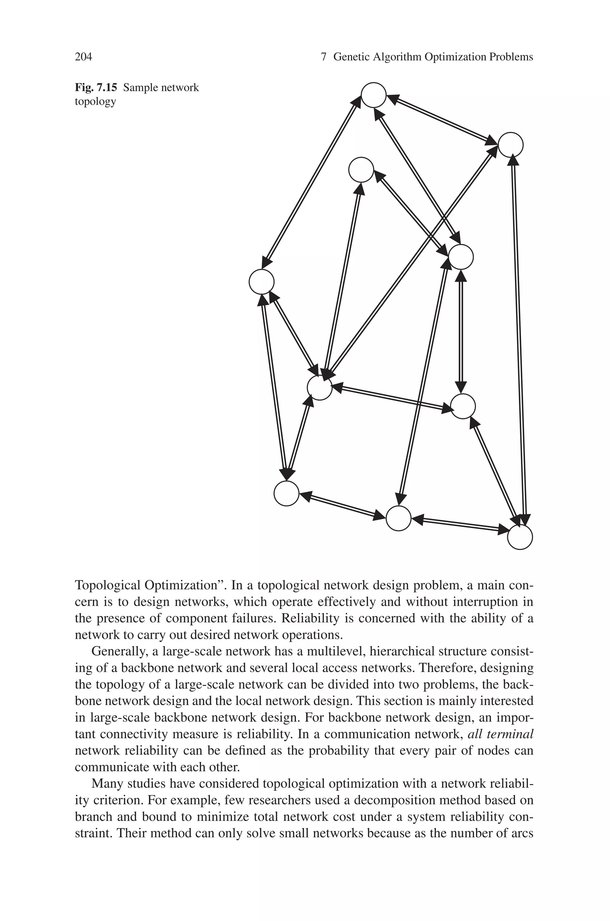
![206 7 Genetic Algorithm Optimization Problems
xij ∈ {0, 1} are the decision variables and f(x) is the network reliability. The all-
terminal system reliability of a network is defined to be the probability that every
pair of nodes can communicate with each other. At any instant of time, only some
arcs of G may be operational. A state of G is a sub-graph (N, L) with L ∈ L, where
L is the set of operational arcs. An operational state is generally called a pathset, and
a minimal operational state is a min-path. A failed state L is called L L (cutset)
and when L is a maximal failed state, L L is a min-cut. The reliability of G,
RelK(G), is the k-terminal reliability: If K = N, this is the all terminal reliability,
Rel(G). It is easy to formulate a network in state L ⊆ L, with reliability as follows:
#
pe
#
qe where L is the set of operational arcs.
e ∈ L
e ∈ ( LL
) (7.30)
Summing this state occurrence probability over all operational states gives the net-
work system reliability. There are basically two approaches to network system relia-
bility calculation; simulation and analytic. All known analytic methods have worst-
case computation times, which grow exponentially with the size of the network.
Monte Carlo simulation methods, for which computation time grows only slightly
faster than linear with network size, have been the method of choice for more than
trivial sized networks. In this section, Monte Carlo simulation technique is used
to predict the network reliability, which substantially reduces the variance of the
estimator when compared to “crude” Monte Carlo. This reduced variance Monte
Carlo is based on a two-tiered hierarchical approach to sampling, which makes use
of how many arcs fail during a given simulation.
7.7.3.2 Genetic Algorithm Approach
A GA is developed as a solution methodology for network topological optimization
with a reliability constraint. In GA, the search space is composed of possible solu-
tions to the problem; each represented as some convenient data structure, referred to
as the chromosome. Each chromosome has an associated objective function value,
called the fitness value. A good chromosome is the one that has a high fitness value.
A set of chromosomes together with their associated fitness values is called the
population. This population, at a given stage of the GA, is referred to as a generation.
In a conventional GA, candidate solutions are represented by strings of numbers
using a binary or non-binary alphabet. The present algorithm uses a binary coding
structure for representing candidate solutions. A binary set is used to represent arcs,
where the maximum number of non-redundant, undirected arcs for a network of
n nodes is given by (n-1)n/2. For example, a simple network whose base graph
consists of 5 nodes and 10 possible links can be represented by:
[ 1 1 0 1 1 0 1 1 0 1 ]
[ x12, x13, x14, x15, x23, x24, x25, x34, x35, x45 ]](https://image.slidesharecdn.com/s-220425101513/75/S-N-Sivanandam-S-N-Deepa-Introduction-to-Genetic-Algorithms-2008-ISBN-3540731894-pdf-219-2048.jpg)
![7.7 Network Design and Routing Problems 207
where, xij represents a link connecting two nodes i and j. If xij is equal to 1, there is a
connection between these two nodes. If xij is equal to 0, then there is no connection.
The initial population, which consists of a set of feasible solutions (2- connected
networks) is generated in a random fashion. For determining this initial population,
a number of experiments were carried out. A candidate network consists of some
randomly selected arcs between nodes. The selection of the probability values,
which are used in deciding whether an arc exists or not was an important step to
generate the initial population. In an experimental design with 10, 20 and 30 nodes,
the following characteristics were systematically controlled.
• Arc probabilities between [0, 1], which determines the existence of an arc
between nodes, are selected.
• The system reliability value of each connected network is estimated using Monte
Carlo simulation.
• The probability values of the existence of arcs and the corresponding network
reliability values are compiled.
The aim was to determine the intervals of the probability values, which result highly
reliable networks. Any initial population can then be generated by using probabili-
ties within these intervals. Table 7.4 shows the resulting probability intervals from
the experiments described above which were used for the initial populations.
The choice of parameters for GAs can have a significant effect on performance
of the algorithm. Parameter values were investigated by running the GA with dif-
ferent population sizes (10, 20, 30), crossover rates (0.55, 0.65, 0.75, 0.85, 0.95)
and mutation rates (0.01, 0.05, 0.09, 0.10). It was found that the best results were:
population size = 20, crossover rate = 0.95 and mutation rate = 0.05.
The objective function is the sum of the total cost for all arcs in the network plus a
quadratic penalty function, which is applied when the network reliability prediction
does not meet the network reliability requirement (i.e., infeasible). The objective of
the penalty function is to lead the optimization algorithm to feasible solutions. It
was important to allow infeasible solutions into the population because good solu-
tions are often the result of breeding between feasible and infeasible solution. The
objective function is,
Z =
i
j
cijXij + δ(ε(Rel(G)-p0))2
, i = 1, . . ., n-1; j = i + 1, . . ., n
(7.31)
where cij, xij and p0 were previously defined, Rel(G) equals f(x) (network reliabil-
ity), ε is the maximum value of cij and δ = 0 if Rel (G) is ≥ p0 and δ = 1 if Rel(G)
p0. The fitness is chosen to be (Zmax–Z) where Zmax is a constant, which is
Table 7.4 Probability values used to generate the initial population
Number of nodes (n) Probability of an arc
10 (0.15–0.60)
20 (0.15–0.50)
30 (0.10–0.30)](https://image.slidesharecdn.com/s-220425101513/75/S-N-Sivanandam-S-N-Deepa-Introduction-to-Genetic-Algorithms-2008-ISBN-3540731894-pdf-220-2048.jpg)
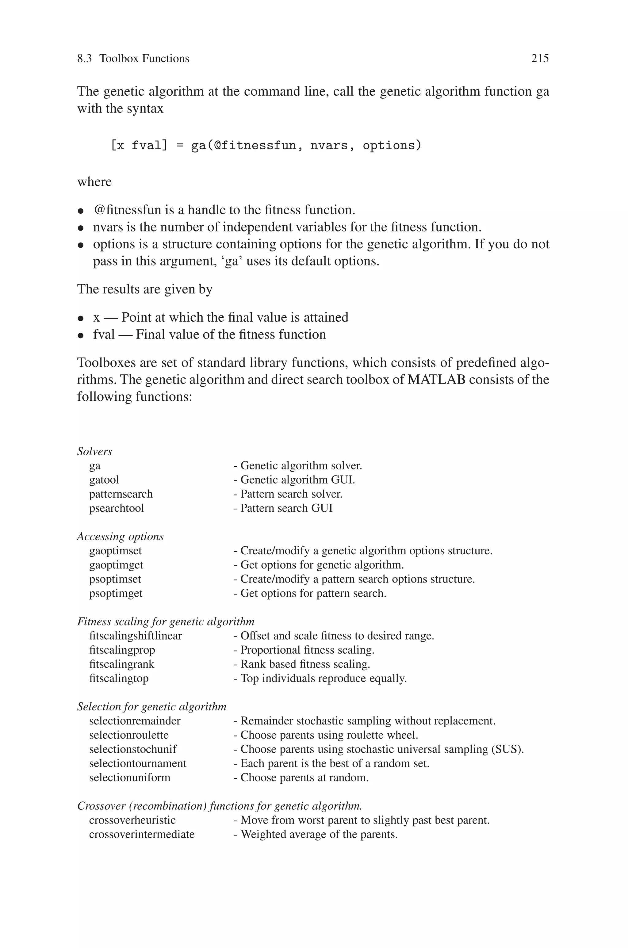
![8.3 Toolbox Functions 215
The genetic algorithm at the command line, call the genetic algorithm function ga
with the syntax
[x fval] = ga(@fitnessfun, nvars, options)
where
• @fitnessfun is a handle to the fitness function.
• nvars is the number of independent variables for the fitness function.
• options is a structure containing options for the genetic algorithm. If you do not
pass in this argument, ‘ga’ uses its default options.
The results are given by
• x — Point at which the final value is attained
• fval — Final value of the fitness function
Toolboxes are set of standard library functions, which consists of predefined algo-
rithms. The genetic algorithm and direct search toolbox of MATLAB consists of the
following functions:
Solvers
ga - Genetic algorithm solver.
gatool - Genetic algorithm GUI.
patternsearch - Pattern search solver.
psearchtool - Pattern search GUI
Accessing options
gaoptimset - Create/modify a genetic algorithm options structure.
gaoptimget - Get options for genetic algorithm.
psoptimset - Create/modify a pattern search options structure.
psoptimget - Get options for pattern search.
Fitness scaling for genetic algorithm
fitscalingshiftlinear - Offset and scale fitness to desired range.
fitscalingprop - Proportional fitness scaling.
fitscalingrank - Rank based fitness scaling.
fitscalingtop - Top individuals reproduce equally.
Selection for genetic algorithm
selectionremainder - Remainder stochastic sampling without replacement.
selectionroulette - Choose parents using roulette wheel.
selectionstochunif - Choose parents using stochastic universal sampling (SUS).
selectiontournament - Each parent is the best of a random set.
selectionuniform - Choose parents at random.
Crossover (recombination) functions for genetic algorithm.
crossoverheuristic - Move from worst parent to slightly past best parent.
crossoverintermediate - Weighted average of the parents.](https://image.slidesharecdn.com/s-220425101513/75/S-N-Sivanandam-S-N-Deepa-Introduction-to-Genetic-Algorithms-2008-ISBN-3540731894-pdf-227-2048.jpg)
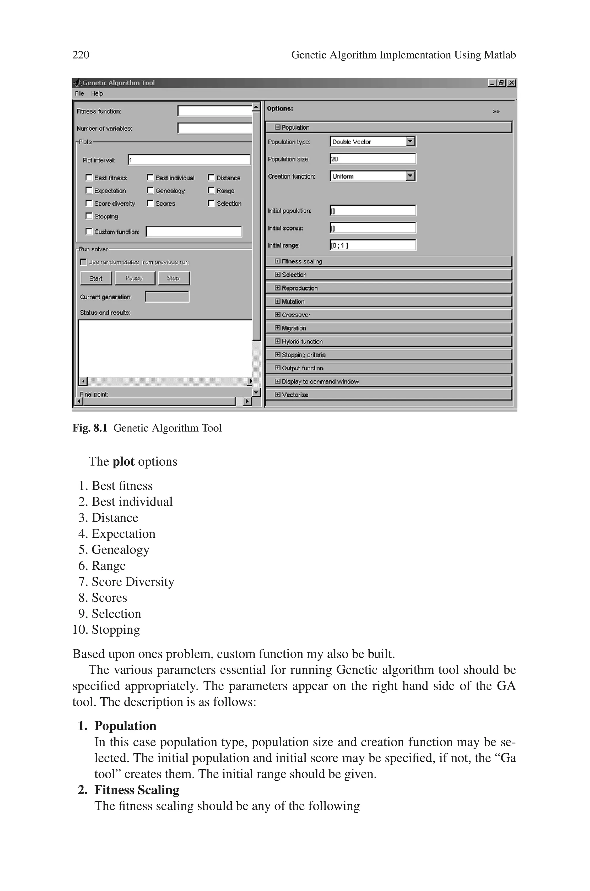


![224 Genetic Algorithm Implementation Using Matlab
The running process may be temporarily stopped using “Pause” option and
permanently stopped using “Stop” option. The “current generation” will be dis-
played during the iteration. Once the iterations are completed, the status and re-
sults will be displayed. Also the “final point” for the fitness function will be
displayed.
8.5 Solved Problems using MATLAB
Problem 1
Write a MATLAB program for maximizing f(x) = x2 using genetic algorithm,
where x ranges from 0 to 31. Perform 4 iterations.
Note
In MATLAB % indicates comment statement.
Source Code
%program for Genetic algorithm to maximize the function f(x) =xsquare
clear all;
clc;
%x ranges from 0 to 31 2power5 = 32
%five bits are enough to represent x in binary representation
n=input(‘Enter no. of population in each iteration’);
nit=input(‘Enter no. of iterations’);
%Generate the initial population
[oldchrom]=initbp(n,5)
%The population in binary is converted to integer
FieldD=[5;0;31;0;0;1;1]
for i=1:nit
phen=bindecod(oldchrom,FieldD,3); % phen gives the integer value of the
binary population %obtain fitness value
sqx=phen. ∧2;
sumsqx=sum(sqx);
avsqx=sumsqx/n;
hsqx=max(sqx);
pselect=sqx./sumsqx;
sumpselect=sum(pselect);
avpselect=sumpselect/n;
hpselect=max(pselect);
%apply roulette wheel selection](https://image.slidesharecdn.com/s-220425101513/75/S-N-Sivanandam-S-N-Deepa-Introduction-to-Genetic-Algorithms-2008-ISBN-3540731894-pdf-236-2048.jpg)
![228 Genetic Algorithm Implementation Using Matlab
These methods are designed to solve “smooth”, i.e., continuous and differentiable,
minimization problems, as they use derivatives to determine the direction of de-
scent. While using derivatives makes these methods fast and accurate, they often
are not effective when problems lack smoothness, e.g., problems with discontinu-
ous, non-differentiable, or stochastic objective functions. When faced with solving
such non-smooth problems, methods like the genetic algorithm or the more recently
developed pattern search methods, both found in the Genetic Algorithm and Direct
Search Toolbox, are effective alternatives.
Source Code
clear all; close all;format compact
Objfcn = @nonSmoothFcn; %Handle to the objective function
X0 = [2 -2]; % Starting point
range = [-6 6;-6 6]; %Range used to plot the objective function
rand(‘state’,0); %Reset the state of random number generators
randn(‘state’,0);
type nonSmoothFcn.m % Non-smooth Objective Function
showNonSmoothFcn(Objfcn,range);
set(gca,‘CameraPosition’,[-36.9991 62.6267 207.3622]);
set(gca,‘CameraTarget’,[0.1059 -1.8145 22.3668])
set(gca,‘CameraViewAngle’,6.0924)
%Plot of the starting point (used by the PATTERNSEARCH solver)
plot3(X0(1),X0(2),feval(Objfcn,X0),‘or’,‘MarkerSize’,10,‘MarkerFaceColor’,‘r’);
fig = gcf;
% Minimization Using The Genetic Algorithm
FitnessFcn = @nonSmoothFcn;
numberOfVariables = 2;
optionsGA = gaoptimset(’PlotFcns’,@gaplotbestfun,‘PlotInterval’,5, ...
‘PopInitRange’,[-5;5]);
% We run GA with the options ‘optionsGA’ as the third argument.
[Xga,Fga] = ga(FitnessFcn,numberOfVariables,optionsGA)
% Plot the final solution
figure(fig)
hold on;
plot3(Xga(1),Xga(2),Fga,‘vm’,‘MarkerSize’,10,‘MarkerFaceColor’,‘m’);
hold off;
fig = gcf;
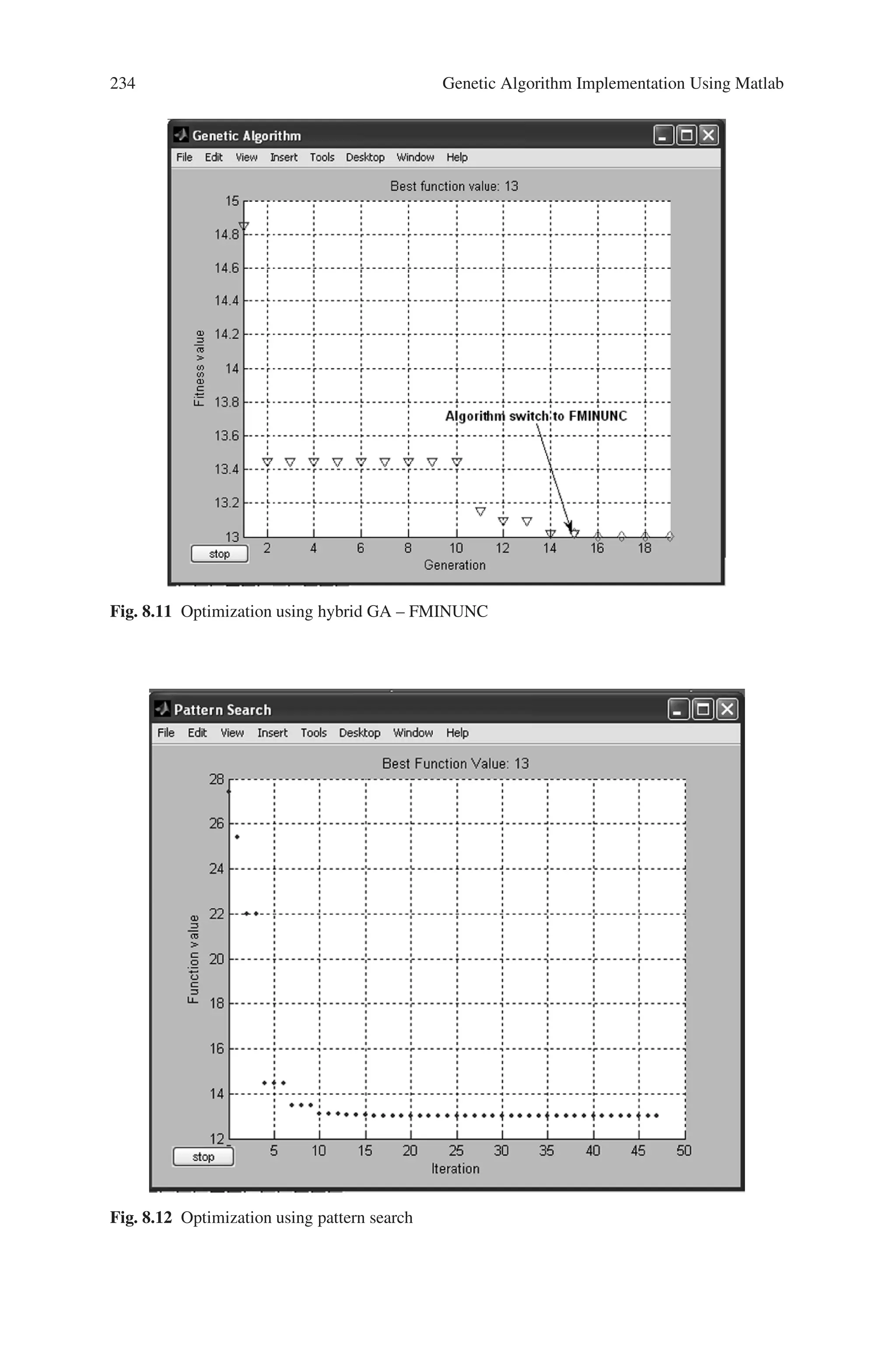
% The optimum is at x* = (−4.7124, 0.0). GA found the point % (−4.7775,0.0481)
near the optimum, but could not get closer with the default stopping criteria. By
changing the stopping criteria, we might find a more accurate solution, but it may
take many more function evaluations to reach x* = (−4.7124, 0.0). Instead, we can
use a more efficient local search that starts where GA left off. The hybrid function
field in GA provides this feature automatically.](https://image.slidesharecdn.com/s-220425101513/75/S-N-Sivanandam-S-N-Deepa-Introduction-to-Genetic-Algorithms-2008-ISBN-3540731894-pdf-240-2048.jpg)
![8.5 Solved Problems using MATLAB 229
% Minimization Using A Hybrid Function
% Our choices are FMINSEARCH, PATTERNSEARCH, or FMINUNC. Since this
optimization example is smooth near the optimizer, we can use the FMINUNC func-
tion from the Optimization toolbox as our hybrid function as this is likely to be the
most efficient. Since FMINUNC has its own options structure, we provide it as an
additional argument when specifying the hybrid function.
% Run GA-FMINUNC Hybrid
optHybrid = gaoptimset(optionsGA,‘Generations’,15, ‘PlotInterval’,1,...
‘HybridFcn’,{@fminunc,optimset(‘OutputFcn’,@fminuncOut)});
[Xhybrid,Fhybrid] = ga(Objfcn,2,optHybrid);
% Plot the final solution
figure(fig);
hold on;
plot3(Xhybrid(1),Xhybrid(2),Fhybrid+1,‘ ∧ c’,‘MarkerSize’,10,
‘MarkerFaceColor’,’c’);
hold off;
disp([‘The norm of |Xga - Xhb| is ’, num2str(norm(Xga-Xhybrid))]);
disp([‘The difference in function values Fga and Fhb is ’,
num2str(Fga - Fhybrid)]);
%% Minimization Using The Pattern Search Algorithm
% To minimize our objective function using the PATTERNSEARCH function, we
need to pass in a function handle to the objective function as well as specifying a
start point as the second argument.
ObjectiveFunction = @nonSmoothFcn;
X0 = [2 -2]; % Starting point
% Some plot functions are selected to monitor the performance of the solver.
optionsPS = psoptimset(’PlotFcns’,@psplotbestf);
% Run pattern search solver
[Xps,Fps] = patternsearch(Objfcn,X0,[],[],[],[],[],[],optionsPS)
% Plot the final solution
figure(fig)
hold on;
plot3(Xps(1),Xps(2),Fps+1,‘*y’,‘MarkerSize’,14,‘MarkerFaceColor’,‘y’);
hold off;
The various functions used in optimization of non-smooth function are a follows:
function [f, g] = nonSmoothFcn(x)
%NONSMOOTHFCN is a non-smooth objective function](https://image.slidesharecdn.com/s-220425101513/75/S-N-Sivanandam-S-N-Deepa-Introduction-to-Genetic-Algorithms-2008-ISBN-3540731894-pdf-241-2048.jpg)
![230 Genetic Algorithm Implementation Using Matlab
for i = 1:size(x,1)
if x(i,1) -7
f(i) = (x(i,1))∧2 + (x(i,2))∧2 ;
elseif x(i,1) -3
f(i) = -2*sin(x(i,1)) - (x(i,1)*x(i,2)∧2)/10 + 15 ;
elseif x(i,1) 0
f(i) = 0.5*x(i,1)∧2 + 20 + abs(x(i,2))+ patho(x(i,:));
elseif x(i,1) = 0
f(i) = .3*sqrt(x(i,1)) + 25 +abs(x(i,2)) + patho(x(i,:));
end
end
%Calculate gradient
g = NaN;
if x(i,1) -7
g = 2*[x(i,1); x(i,2)];
elseif x(i,1) -3
g = [-2*cos(x(i,1))-(x(i,2)∧2)/10; -x(i,1)*x(i,2)/5];
elseif x(i,1) 0
[fp,gp] = patho(x(i,:));
if x(i,2) 0
g = [x(i,1)+gp(1); 1+gp(2)];
elseif x(i,2) 0
g = [x(i,1)+gp(1); -1+gp(2)];
end
elseif x(i,1) 0
[fp,gp] = patho(x(i,:));
if x(i,2) 0
g = [.15/sqrt(x(i,1))+gp(1); 1+ gp(2)];
elseif x(i,2) 0
g = [.15/sqrt(x(i,1))+gp(1); -1+ gp(2)];
end
end
function [f,g] = patho(x)
Max = 500;
f = zeros(size(x,1),1);
g = zeros(size(x));
for k = 1:Max %k
arg = sin(pi*k∧2*x)/(pi*k∧2);
f = f + sum(arg,2);
g = g + cos(pi*k∧2*x);
end
function showNonSmoothFcn(fcn,range)
if(nargin == 0)
fcn = @rastriginsfcn;
range = [-5,5;-5,5];](https://image.slidesharecdn.com/s-220425101513/75/S-N-Sivanandam-S-N-Deepa-Introduction-to-Genetic-Algorithms-2008-ISBN-3540731894-pdf-242-2048.jpg)
![8.5 Solved Problems using MATLAB 231
end
pts = 25;
span = diff(range’)/(pts - 1);
x = range(1,1): span(1) : range(1,2);
y = range(2,1): span(2) : range(2,2);
pop = zeros(pts * pts,2);
k = 1;
for i = 1:pts
for j = 1:pts
pop(k,:) = [x(i),y(j)];
k = k + 1;
end
end
values = feval(fcn,pop);
values = reshape(values,pts,pts);
surf(x,y,values)
shading interp
light
lighting phong
hold on
contour(x,y,values)
rotate3d
view(37,60)
%Annotations
figure1 = gcf;
% Create arrow
annotation1 = annotation(figure1,’arrow’,[0.5946 0.4196],[0.9024 0.6738]);
% Create textbox
annotation2 = annotation(...
figure1,‘textbox’,...
‘Position’,[0.575 0.9071 0.1571 0.07402],...
‘FitHeightToText’,’off’,...
‘FontWeight’,’bold’,...
‘String’,{’Start point’});
% Create textarrow
annotation3 = annotation(...
figure1,‘textarrow’,...
[0.3679 0.4661],[0.1476 0.3214],...
‘String’,{‘Non-differentiable regions’},...
‘FontWeight’,‘bold’);
% Create arrow
annotation4 = annotation(figure1,‘arrow’,[0.1196 0.04107],[0.1381 0.5429]);
% Create textarrow
annotation5 = annotation(...
figure1,‘textarrow’,...
[0.7411 0.5321],[0.05476 0.1381],...](https://image.slidesharecdn.com/s-220425101513/75/S-N-Sivanandam-S-N-Deepa-Introduction-to-Genetic-Algorithms-2008-ISBN-3540731894-pdf-243-2048.jpg)
![232 Genetic Algorithm Implementation Using Matlab
‘LineWidth’,2,...
‘Color’,[1 0 0],...
‘String’,{’Smooth region’},...
‘FontWeight’,’bold’,...
‘TextLineWidth’,2,...
‘TextEdgeColor’,[1 0 0]);
% Create arrow
annotation6 = annotation(...
figure1,‘arrow’,...
[0.8946 0.9179],[0.05714 0.531],...
‘Color’,[1 0 0]);
function stop = fminuncOut(x,optimvalues, state)
persistent fig gaIter
stop = false;
switch state
case ‘init’
fig = findobj(0,‘type’,‘figure’,‘name’,‘Genetic Algorithm’);
limits = get(gca,‘XLim’);
gaIter = limits(2);
hold on;
case ‘iter’
set(gca,‘Xlim’, [1 optimvalues.iteration + gaIter]);
fval = optimvalues.fval;
iter = gaIter + optimvalues.iteration;
plot(iter,fval,’dr’)
title([‘Best function value: ’,num2str(fval)],‘interp’,‘none’)
case ‘done’
fval = optimvalues.fval;
iter = gaIter + optimvalues.iteration;
title([‘Best function value: ’,num2str(fval)],‘interp’,‘none’)
% Create textarrow
annotation1 = annotation(...
gcf,‘textarrow’,...
[0.6643 0.7286],[0.3833 0.119],...
‘String’,{‘Algorithm switch to FMINUNC’},...
‘FontWeight’,‘bold’);
hold off
end
Output
Optimization terminated: maximum number of generations exceeded.
Xga =
-4.7775 0.0481](https://image.slidesharecdn.com/s-220425101513/75/S-N-Sivanandam-S-N-Deepa-Introduction-to-Genetic-Algorithms-2008-ISBN-3540731894-pdf-244-2048.jpg)
![8.5 Solved Problems using MATLAB 235
Problem 3
Find a minimum of a stochastic objective function using PATTERNSEARCH func-
tion in the Genetic Algorithm and Direct Search Toolbox.
Source Code
% Pattern search optimization solver
format compact
X0 = [2.5 -2.5]; %Starting point.
LB = [-5 -5]; %Lower bound
UB = [5 5]; %Upper bound
range = [LB(1) UB(1); LB(2) UB(2)];
Objfcn = @smoothFcn; %Handle to the objective function.
% Plot the smooth objective function
clf;showSmoothFcn(Objfcn,range); hold on;
title(‘Smooth objective function’)
plot3(X0(1),X0(2),feval(Objfcn,X0)+30,‘om’,‘MarkerSize’,12, ...
‘MarkerFaceColor’,‘r’); hold off;
set(gca,‘CameraPosition’,[-31.0391 -85.2792 -281.4265]);
set(gca,‘CameraTarget’,[0 0 -50])
set(gca,‘CameraViewAngle’,6.7937)
fig = gcf;
%% Run FMINCON on smooth objective function
% The objective function is smooth (twice continuously differentiable). Solving the
optimization problem using FMINCON function from the Optimization Toolbox.
FMINCON finds a constrained minimum of a function of several variables. This
function has a unique minimum at the point x∗ = (−5.0, −5) where it has a function
value f(x∗) = −250.
% Set options to display iterative results.
options = optimset(‘Display’,‘iter’,‘OutputFcn’,@fminuncOut1);
[Xop,Fop] = fmincon(Objfcn,X0,[],[],[],[],LB,UB,[],options)
figure(fig);
hold on;
%Plot the final point
plot3(Xop(1),Xop(2),Fop,‘dm’,‘MarkerSize’,12,‘MarkerFaceColor’,‘m’);
hold off;
% Stochastic objective function The objective function is same as the previous
function and some noise](https://image.slidesharecdn.com/s-220425101513/75/S-N-Sivanandam-S-N-Deepa-Introduction-to-Genetic-Algorithms-2008-ISBN-3540731894-pdf-247-2048.jpg)
![236 Genetic Algorithm Implementation Using Matlab
% added to it.
%Reset the state of random number generators
randn(‘state’,0);
noise = 8.5;
Objfcn = @(x) smoothFcn(x,noise); %Handle to the objective function.
%Plot the objective function (non-smooth)
figure;
for i = 1:6
showSmoothFcn(Objfcn,range);
title(‘Stochastic objective function’)
set(gca,‘CameraPosition’,[-31.0391 -85.2792 -281.4265]);
set(gca,‘CameraTarget’,[0 0 -50])
set(gca,‘CameraViewAngle’,6.7937)
drawnow; pause(0.2)
end
fig = gcf;
%% Run FMINCON on stochastic objective function
options = optimset(‘Display’,‘iter’);
[Xop,Fop] = fmincon(Objfcn,X0,[],[],[],[],LB,UB,[],options)
figure(fig);
hold on;
plot3(X0(1),X0(2),feval(Objfcn,X0)+30,‘om’,‘MarkerSize’,16,
‘MarkerFaceColor’,‘r’);
plot3(Xop(1),Xop(2),Fop,‘dm’,‘MarkerSize’,12,‘MarkerFaceColor’,‘m’);
%% Run PATTERNSEARCH. A pattern search algorithm does not require any
derivative information of the objective function to find an optimal point.
PSoptions = psoptimset(‘Display’,‘iter’,‘OutputFcn’,@psOut);
[Xps,Fps] = patternsearch(Objfcn,X0,[],[],[],[],LB,UB,PSoptions)
figure(fig);
hold on;
plot3(Xps(1),Xps(2),Fps,‘pr’,‘MarkerSize’,18,‘MarkerFaceColor’,‘r’);
hold off
The various functions used in the above program are as follows:
function y = smoothFcn(z,noise)
% Objective function
if nargin 2
noise = 0;
end
LB = [-5 -5]; %Lower bound
UB = [5 5]; %Upper bound
y = zeros(1,size(z,1));
for i = 1:size(z,1)](https://image.slidesharecdn.com/s-220425101513/75/S-N-Sivanandam-S-N-Deepa-Introduction-to-Genetic-Algorithms-2008-ISBN-3540731894-pdf-248-2048.jpg)
![8.5 Solved Problems using MATLAB 237
x = z(i,:);
if any(xLB) || any(xUB)
y(i) = Inf;
else
y(i) = x(1)∧3 - x(2)∧2 + ...
100*x(2)/(10+x(1)) + noise*randn;
end
end
function showSmoothFcn(fcn,range)
pts = 100;
span = diff(range’)/(pts - 1);
x = range(1,1): span(1) : range(1,2);
y = range(2,1): span(2) : range(2,2);
pop = zeros(pts * pts,2);
k = 1;
for i = 1:pts
for j = 1:pts
pop(k,:) = [x(i),y(j)];
k = k + 1;
end
end
values = feval(fcn,pop);
values = reshape(values,pts,pts);
clf;
surf(x,y,values)
shading interp
light
lighting phong
hold on
rotate3d
view(37,60)
set(gcf,‘Renderer’,‘opengl’);
set(gca,‘ZLimMode’,‘manual’);
function stop = fminuncOut1(X, optimvalues, state)
stop = false;
figure1 = gcf;
if strcmpi(state,‘done’)
annotation1 = annotation(figure1,‘arrow’,[0.7506 0.7014],[0.3797 0.625]);
% Create textbox
annotation2 = annotation(...
figure1,‘textbox’,...
‘Position’,[0.6857 0.2968 0.1482 0.0746],...
‘FontWeight’,‘bold’,...](https://image.slidesharecdn.com/s-220425101513/75/S-N-Sivanandam-S-N-Deepa-Introduction-to-Genetic-Algorithms-2008-ISBN-3540731894-pdf-249-2048.jpg)
![238 Genetic Algorithm Implementation Using Matlab
‘String’,{‘start point’},...
‘FitHeightToText’,‘on’);
% Create arrow
annotation3 = annotation(figure1,‘arrow’,[0.4738 0.3489],[0.1774 0.2358]);
% Create textbox
annotation4 = annotation(...
figure1,‘textbox’,...
‘Position’,[0.4732 0.1444 0.2411 0.06032],...
‘FitHeightToText’,‘off’,...
‘FontWeight’,‘bold’,...
‘String’,{‘FMINCON solution’});
end
function [stop options changed] = psOut(optimvalues,options,flag)
stop = false;
changed = false;
figure1 = gcf;
if strcmpi(flag,‘done’)
% Create textbox
annotation1 = annotation(...
figure1,‘textbox’,...
‘Position’,[0.4679 0.1357 0.3321 0.06667],...
‘FitHeightToText’,‘off’,...
‘FontWeight’,‘bold’,...
‘String’,{‘Pattern Search solution’});
% Create textbox
annotation2 = annotation(...
figure1,‘textbox’,...
‘Position’,[0.5625 0.2786 0.2321 0.06667],...
‘FitHeightToText’,‘off’,...
‘FontWeight’,‘bold’,...
‘String’,{‘FMINCON solution’});
% Create textbox
annotation3 = annotation(...
figure1,‘textbox’,...
‘Position’,[0.3714 0.6905 0.1571 0.06449],...
‘FitHeightToText’,‘off’,...
‘FontWeight’,‘bold’,...
‘String’,{‘Start point’});
% Create arrow
annotation4 = annotation(figure1,‘arrow’,[0.7161 0.6768],[0.3452 0.4732]);
% Create arrow
annotation5 = annotation(figure1,‘arrow’,[0.4697 0.35],[0.1673 0.2119]);
% Create arrow](https://image.slidesharecdn.com/s-220425101513/75/S-N-Sivanandam-S-N-Deepa-Introduction-to-Genetic-Algorithms-2008-ISBN-3540731894-pdf-250-2048.jpg)
![8.5 Solved Problems using MATLAB 239
annotation6 = annotation(figure1,‘arrow’,[0.4523 0.6893],[0.6929 0.6]);
end
Output
In fmincon at 260
In PS at 33
Xop =
-5 -5
Fop =
-250
In fmincon at 260
In PS at 70
Xop =
1.2861 -4.8242
Fop =
-86.0221
Xps =
-5 -5
Fps =
-247.3159
Fig. 8.13 Smooth objective function](https://image.slidesharecdn.com/s-220425101513/75/S-N-Sivanandam-S-N-Deepa-Introduction-to-Genetic-Algorithms-2008-ISBN-3540731894-pdf-251-2048.jpg)
![240 Genetic Algorithm Implementation Using Matlab
Fig. 8.14 Stochastic objective function
Pattern search algorithm is not affected by random noise in the objective func-
tions. Pattern search requires only function value and not the derivatives, hence a
noise (of some uniform kind) may not affect it.
Pattern search requires a lot more function evaluation to find the minima, a cost for
not using the derivatives.
Problem 4
Write a Program to maximize sin(x) within the range 0x3.14
Source Code
%program for Genetic algorithm to maximize the function f(x) =sin(x)
clear all;
clc;
%x ranges from 0 to 3.14
%five bits are enough to represent x in binary representation
n=input(‘Enter no. of population in each iteration’);
nit=input(‘Enter no. of iterations’);
%Generate the initial population
[oldchrom]=initbp(n,5)
%The population in binary is converted to integer
FieldD=[5;0;3.14;0;0;1;1]](https://image.slidesharecdn.com/s-220425101513/75/S-N-Sivanandam-S-N-Deepa-Introduction-to-Genetic-Algorithms-2008-ISBN-3540731894-pdf-252-2048.jpg)
![8.5 Solved Problems using MATLAB 245
X = GA(FITNESSFCN,NVARS) finds the minimum of FITNESSFCN
using GA. NVARS is the dimension (number of design variables) of the
FITNESSFCN.
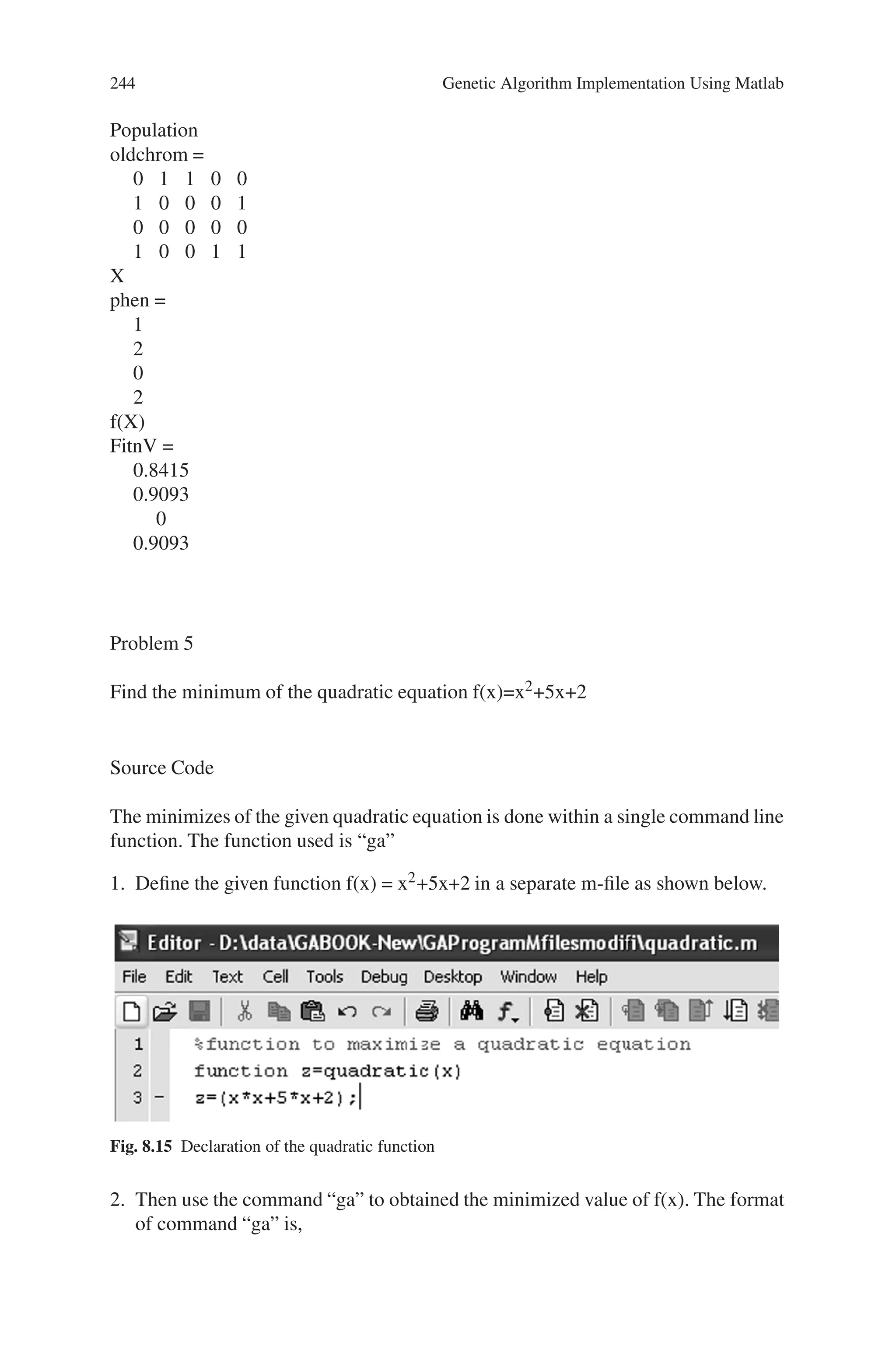
3. Thus the command for the given problem is given by,
x=ga(@quadratic,1)
On running the above command, the output is obtained as given below.
Output
Optimization terminated: maximum number of generations exceeded.
x =
-2.5002
In this case, all the operations are performed with the default setting of the com-
mand “ga”.
In the above case, if the command is specified as,
[x, fval, reason, output, population, scores] = ga(@quadratic,1)
then the output obtained is,
Optimization terminated: maximum number of generations exceeded.
x =
-2.5002
fval =
-4.2500
reason =
Optimization terminated: maximum number of generations exceeded.
output =
randstate: [35x1 double]
randnstate: [2x1 double]
generations: 100
funccount: 2000
message: ‘Optimization terminated: maximum number of generations
exceeded.’
population =
-2.5002
-2.5002
-2.5002
-2.4933
-2.5002
-2.5002
-2.5002](https://image.slidesharecdn.com/s-220425101513/75/S-N-Sivanandam-S-N-Deepa-Introduction-to-Genetic-Algorithms-2008-ISBN-3540731894-pdf-257-2048.jpg)
![8.5 Solved Problems using MATLAB 247
The MATLABtoolbox contains an M-file, rastriginsfcn.m, that computes the values
of Rastrigin’s function.
Source Code
The function is defined as follows:
function Rasfun = rastriginsfcn(pop) %RASTRIGINSFCN Compute the
%“Rastrigin” function.
Rasfun = 10.0 * size(pop,2) + sum(pop .∧2 - 10.0 * cos(2 * pi .* pop),2);
The program for minimizing this function is given as,
%Program to minimize Rastrigins Function
%Depending upon user’s need Options can be specified using the command
‘gaoptimset’. %If
%Options not specified default options are chosen.
options=gaoptimset(‘CrossoverFcn’,@crossoversinglepoint,. . .
‘MutationFcn’,@mutationuniform,‘Plotfcns’,@gaplotbestf)
%Generating the genetic algorithm for 10 variables with the options specified
%above
[x,fval,reason] = ga(@rastriginsFcn,10,options)
Output
options =
PopulationType: ‘doubleVector’
PopInitRange: [2x1 double]
PopulationSize: 20
EliteCount: 2
CrossoverFraction: 0.8000
MigrationDirection: ‘forward’
MigrationInterval: 20
MigrationFraction: 0.2000
Generations: 100
TimeLimit: Inf
FitnessLimit: -Inf
StallGenLimit: 50
StallTimeLimit: 20
InitialPopulation: [ ]
InitialScores: [ ]
PlotInterval: 1
CreationFcn: @gacreationuniform
FitnessScalingFcn: @fitscalingrank](https://image.slidesharecdn.com/s-220425101513/75/S-N-Sivanandam-S-N-Deepa-Introduction-to-Genetic-Algorithms-2008-ISBN-3540731894-pdf-259-2048.jpg)
![248 Genetic Algorithm Implementation Using Matlab
SelectionFcn: @selectionstochunif
CrossoverFcn: @crossoversinglepoint
MutationFcn: @mutationuniform
HybridFcn: [ ]
Display: ‘final’
PlotFcns: @gaplotbestf
OutputFcns: [ ]
Vectorized: ‘off’
Optimization terminated: maximum number of generations exceeded.
x =
Columns 1 through 9
0.9840 0.8061 0.9698 0.0493 0.0070 0.0408 0.0671 0.0970 0.9412
Column 10
0.9848
fval =
15.4207
reason =
Optimization terminated: maximum number of generations exceeded.
Fig. 8.16 Best fitness plot for minimization of Rastrigins function](https://image.slidesharecdn.com/s-220425101513/75/S-N-Sivanandam-S-N-Deepa-Introduction-to-Genetic-Algorithms-2008-ISBN-3540731894-pdf-260-2048.jpg)
![8.5 Solved Problems using MATLAB 249
Problem 7
Write a program to optimize a function f(x1,x2)=3x1+9x2. Set suitable plot
options.
Source Code
The function is defined as follows:
%function to be optimized
function z=twofunc(x)
z=(3*x(1)+9*x(2));
The program code for optimization process is as follows:
%Program to optimize a function with two variables
%Options are set using the command ’gaoptimset’.
clc;
clear all;
options = gaoptimset(’PlotFcns’,. . .
{@gaplotbestf,@gaplotbestindiv,@gaplotexpectation,
@gaplotstopping});
%Generating the genetic algorithm for 2 variables
[x,fval,reason] = ga(@twofunc,2,options)
Output
x =
-14.2395 -24.4720
fval =
-262.9662
reason =
Optimization terminated: maximum number of generations exceeded.](https://image.slidesharecdn.com/s-220425101513/75/S-N-Sivanandam-S-N-Deepa-Introduction-to-Genetic-Algorithms-2008-ISBN-3540731894-pdf-261-2048.jpg)
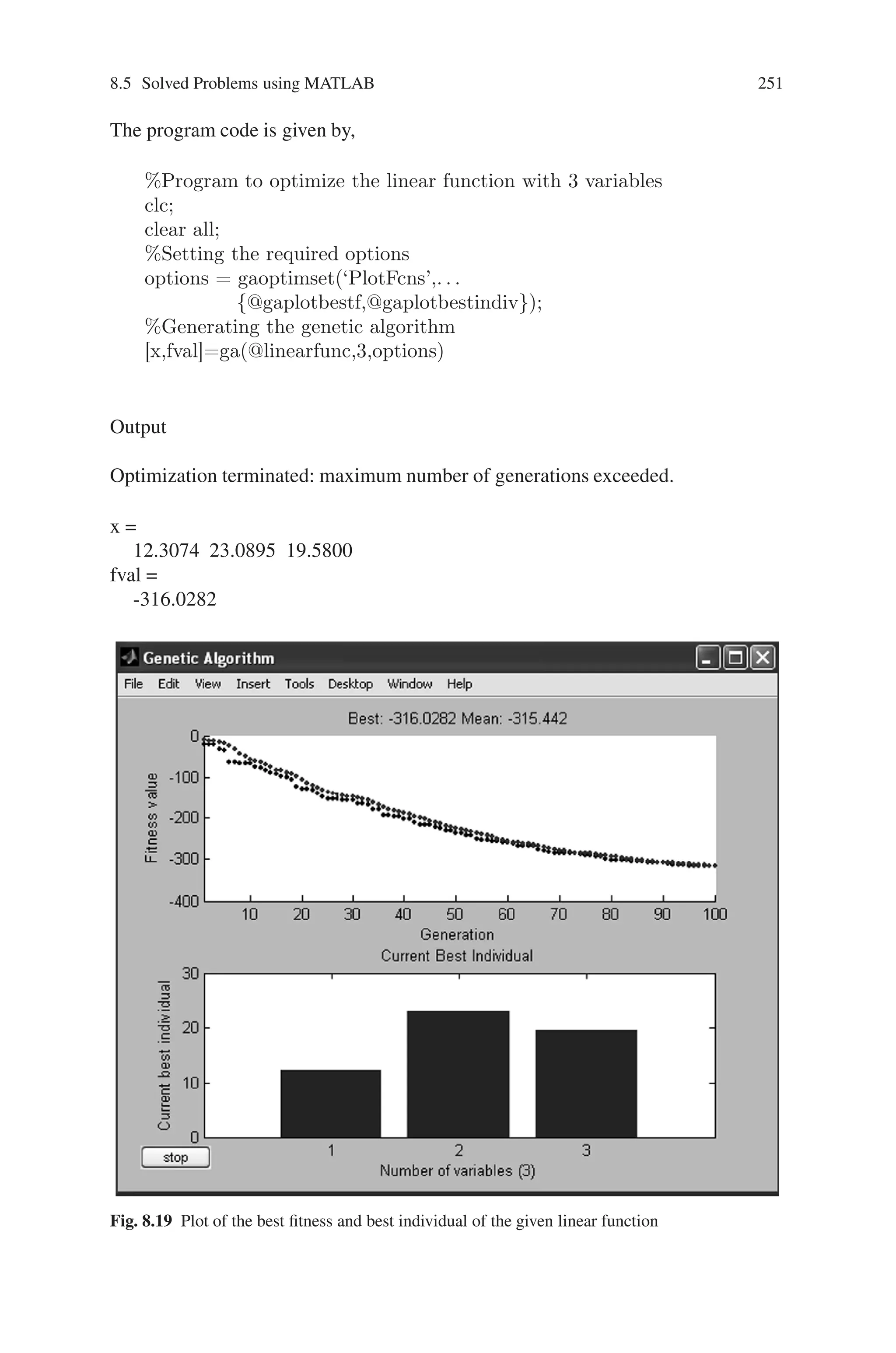
![8.5 Solved Problems using MATLAB 251
The program code is given by,
%Program to optimize the linear function with 3 variables
clc;
clear all;
%Setting the required options
options = gaoptimset(‘PlotFcns’,. . .
{@gaplotbestf,@gaplotbestindiv});
%Generating the genetic algorithm
[x,fval]=ga(@linearfunc,3,options)
Output
Optimization terminated: maximum number of generations exceeded.
x =
12.3074 23.0895 19.5800
fval =
-316.0282
Fig. 8.19 Plot of the best fitness and best individual of the given linear function](https://image.slidesharecdn.com/s-220425101513/75/S-N-Sivanandam-S-N-Deepa-Introduction-to-Genetic-Algorithms-2008-ISBN-3540731894-pdf-263-2048.jpg)
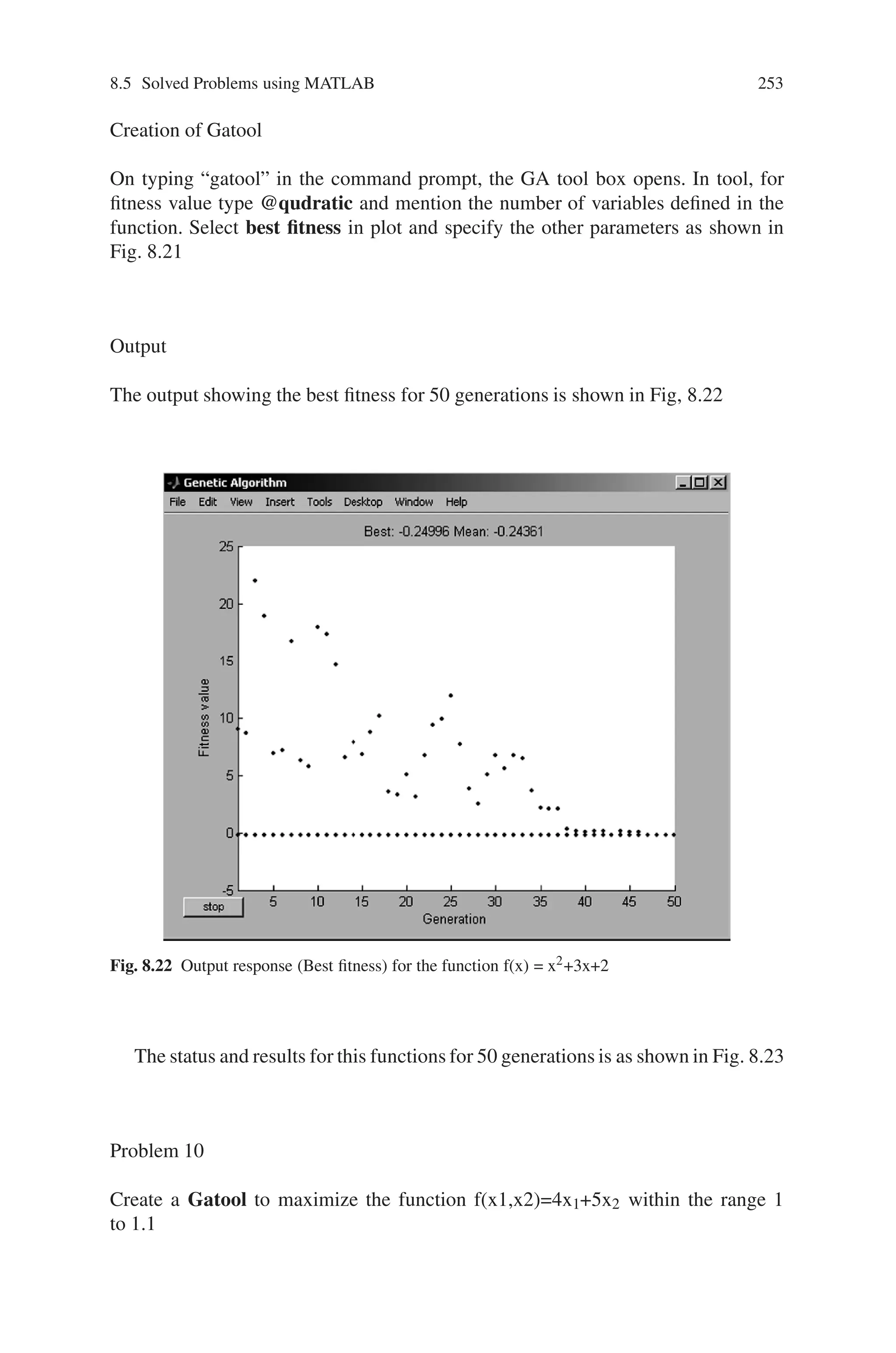
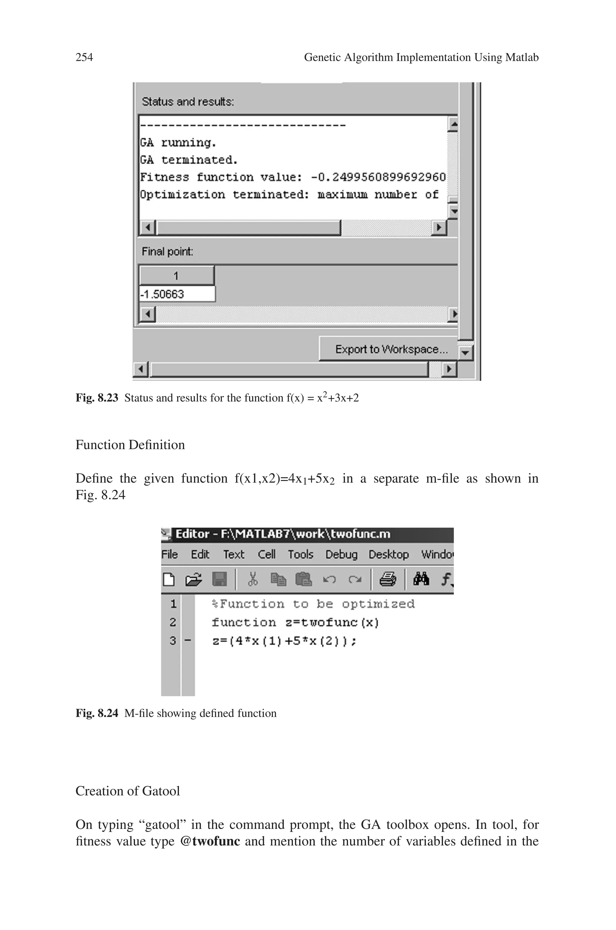
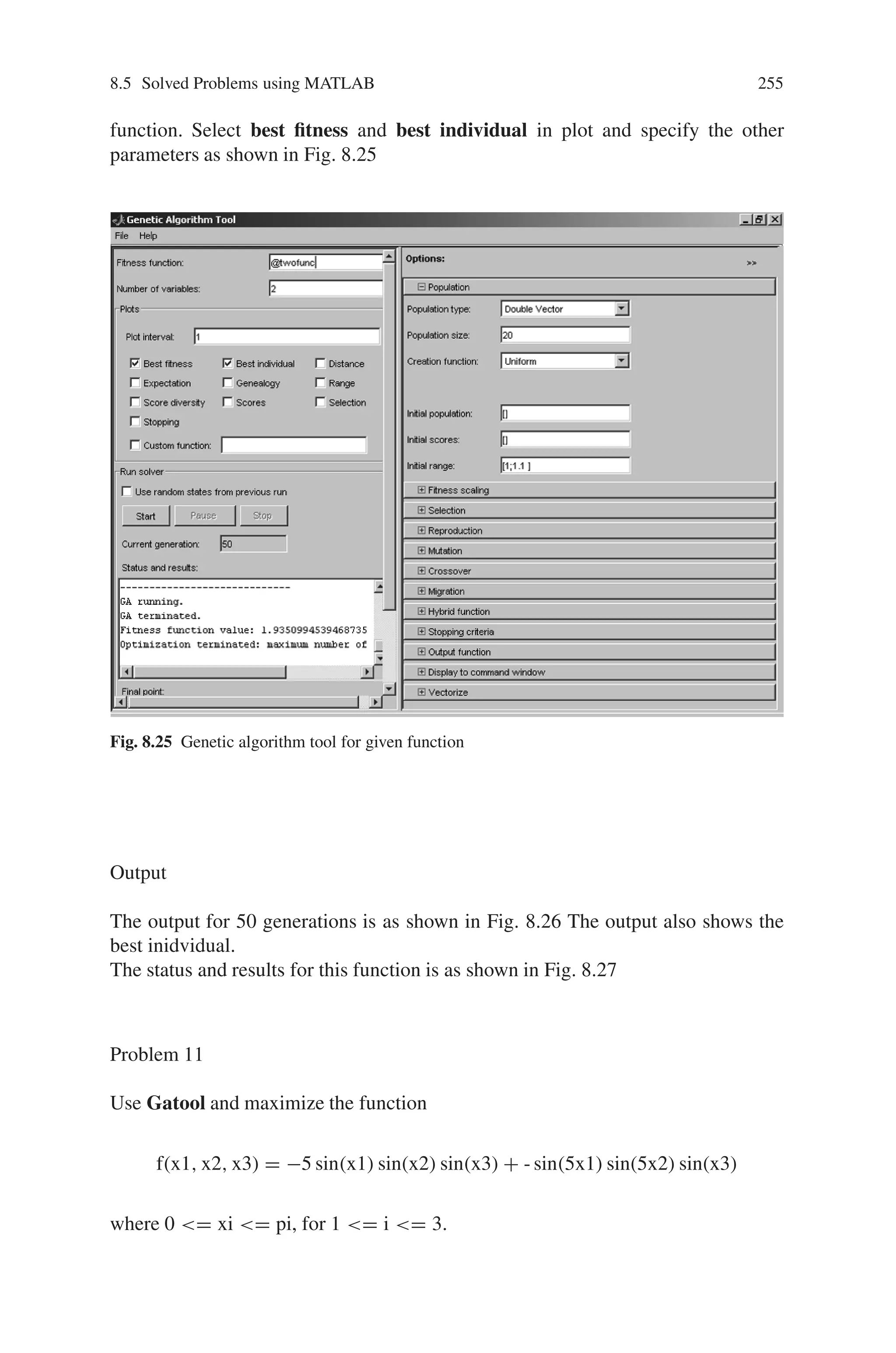
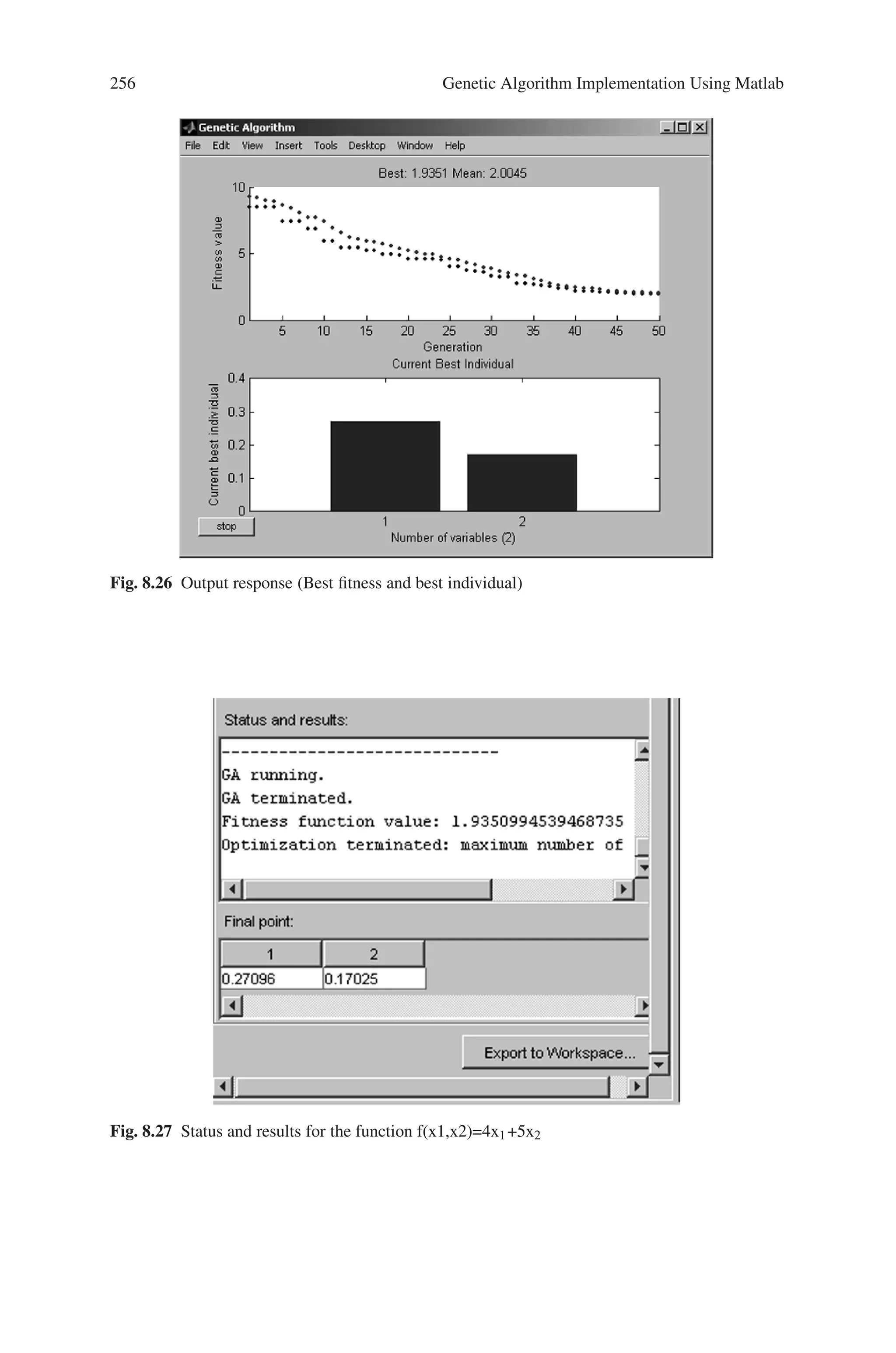
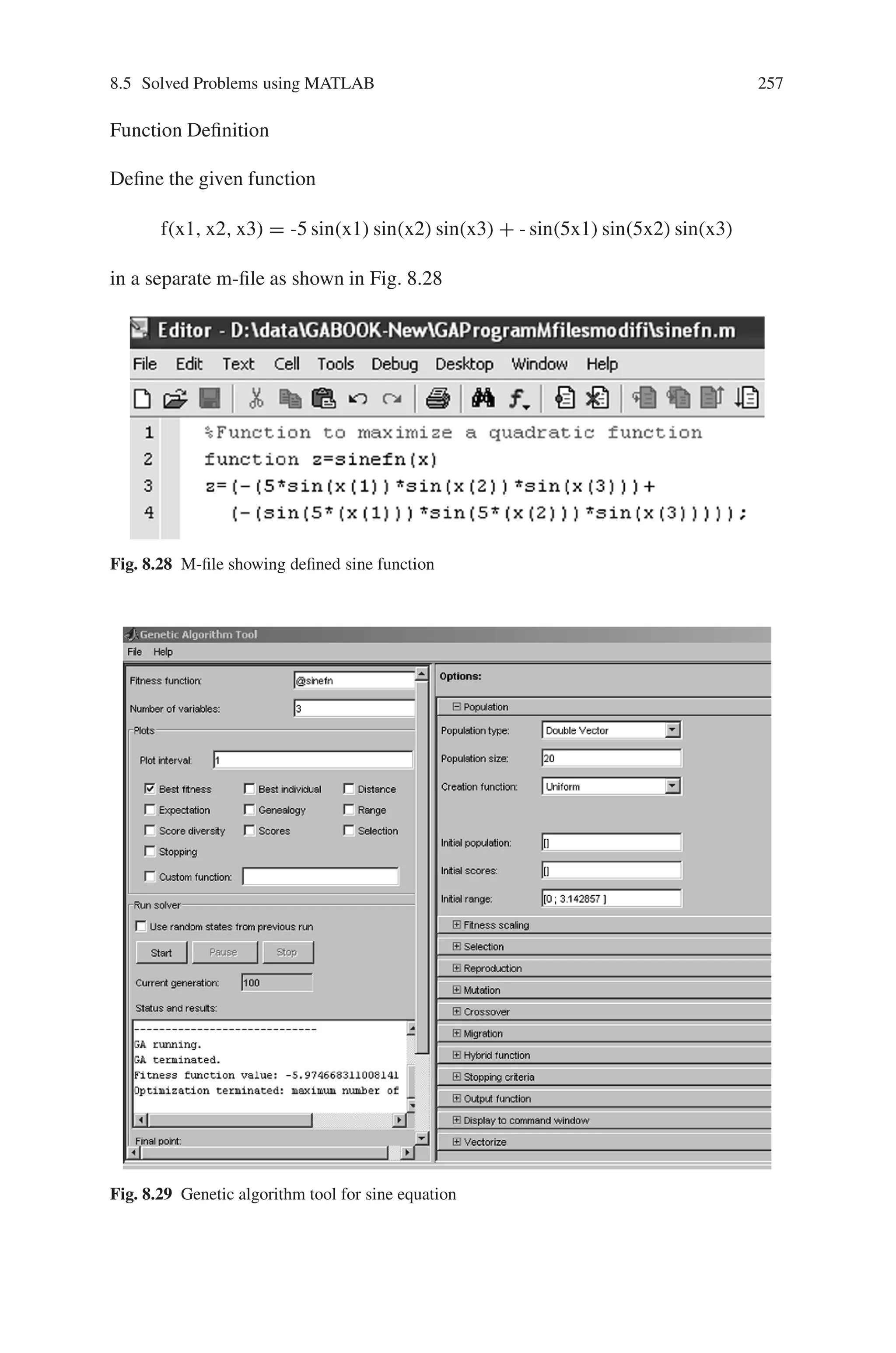
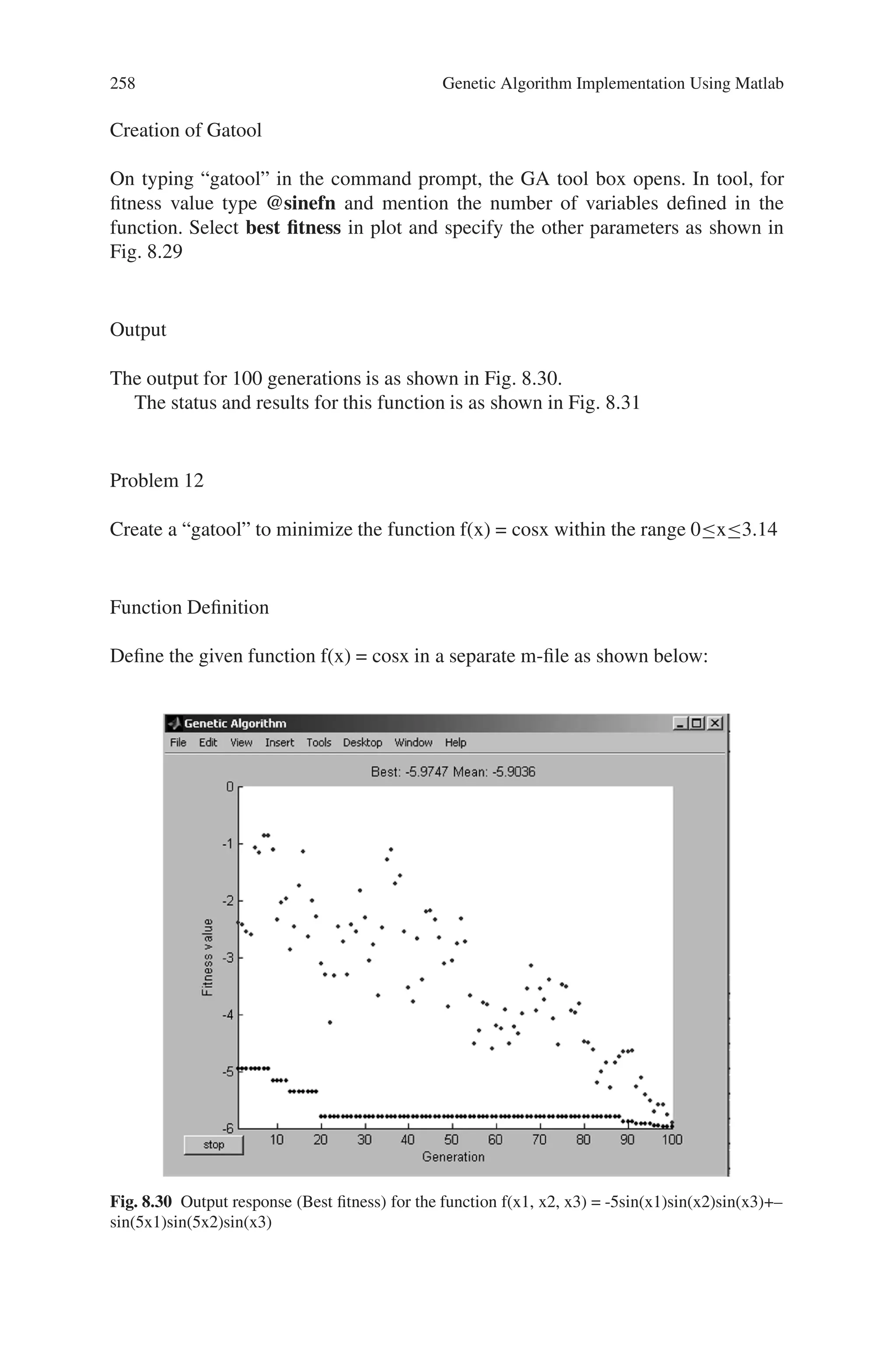
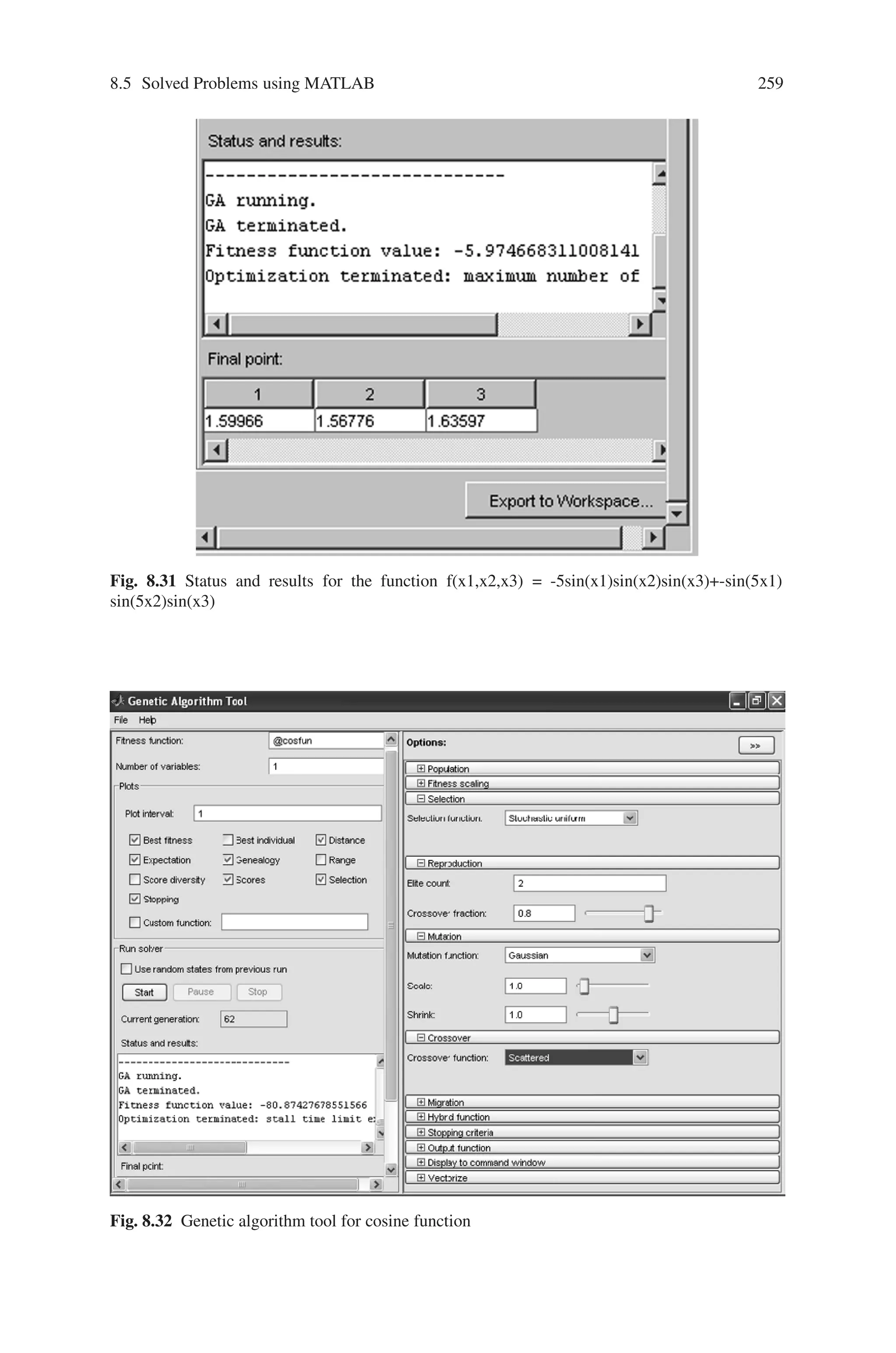
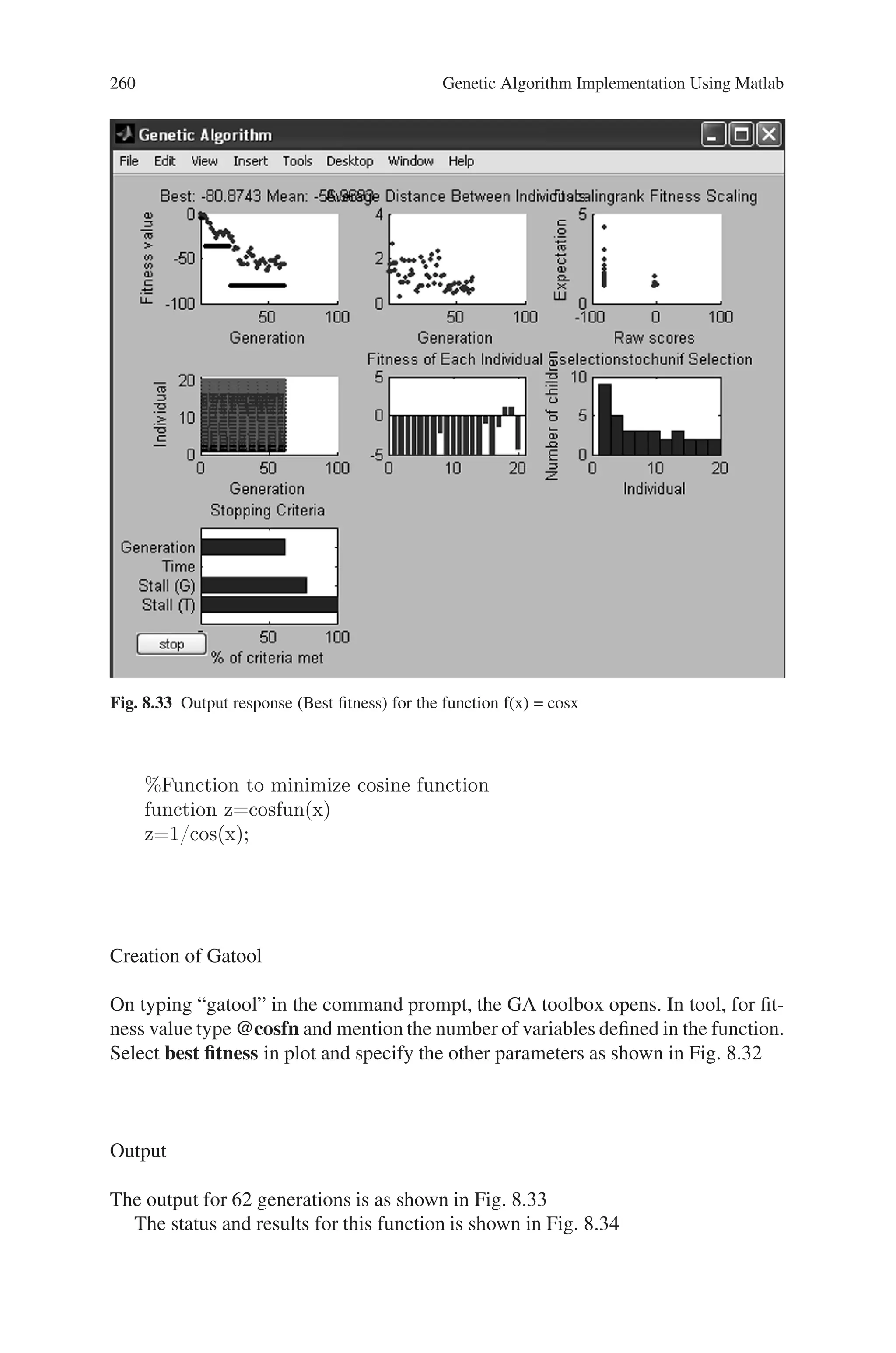
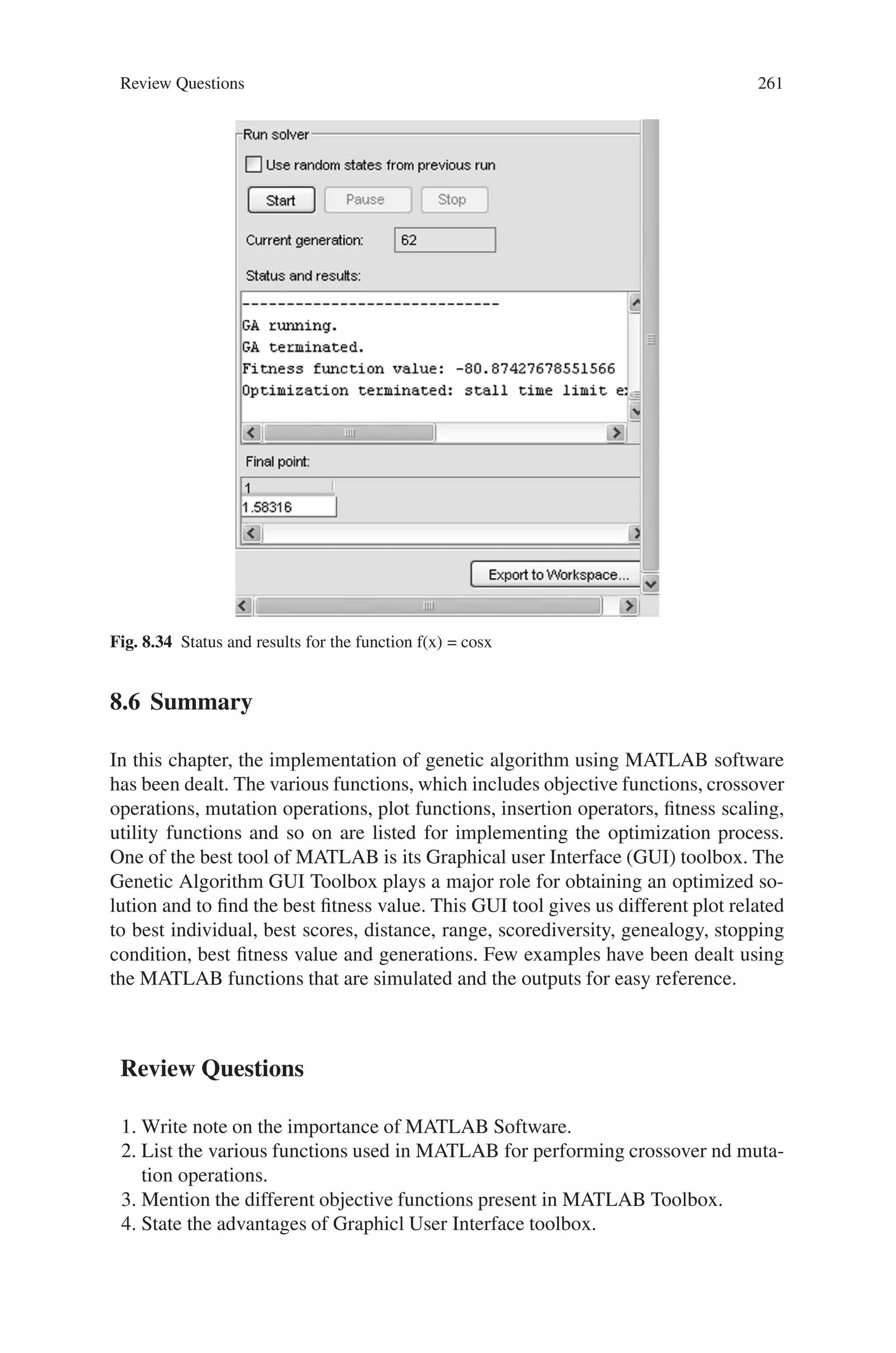
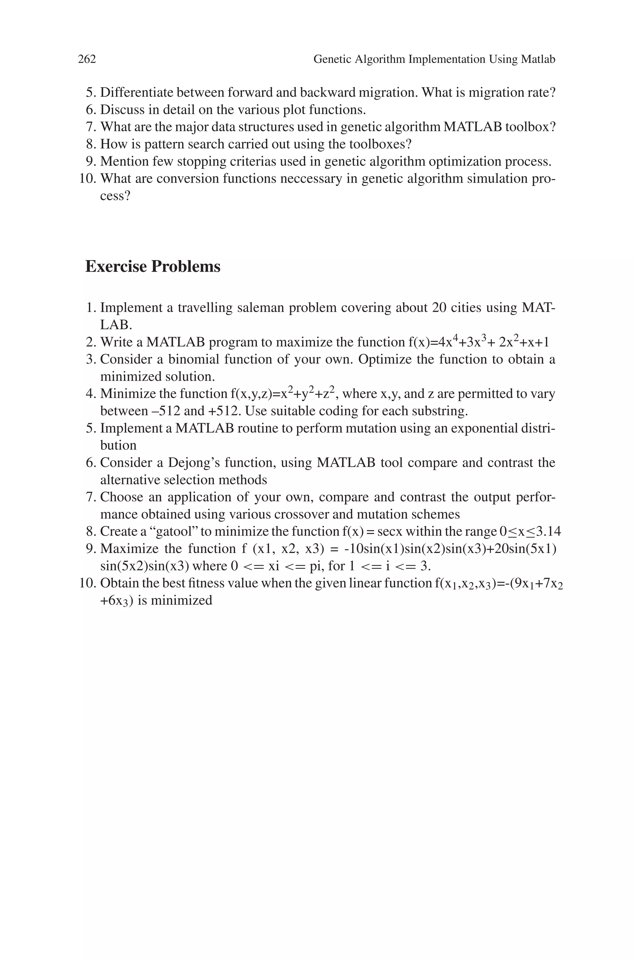
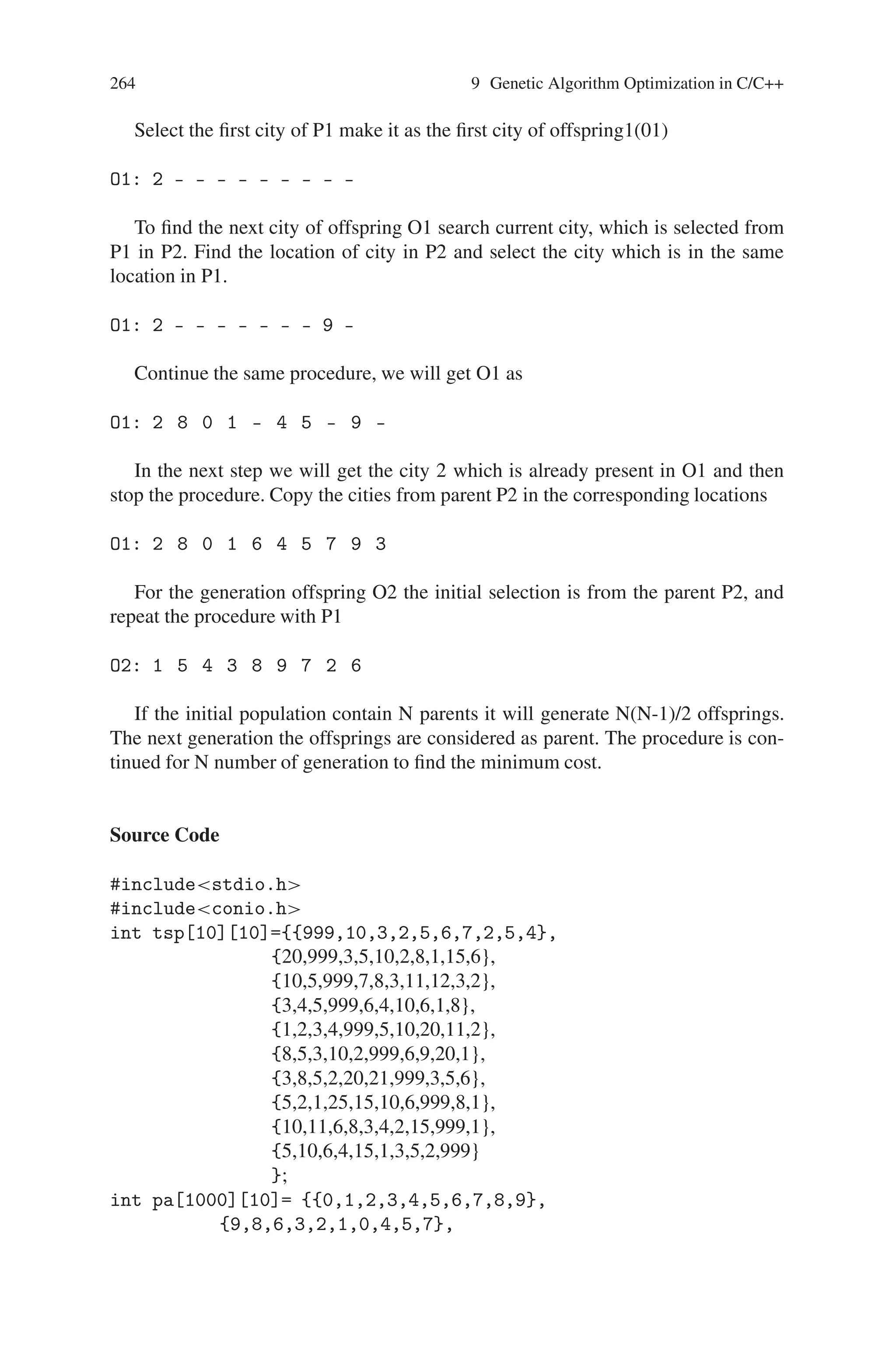
![264 9 Genetic Algorithm Optimization in C/C++
Select the first city of P1 make it as the first city of offspring1(01)
O1: 2 - - - - - - - - -
To find the next city of offspring O1 search current city, which is selected from
P1 in P2. Find the location of city in P2 and select the city which is in the same
location in P1.
O1: 2 - - - - - - - 9 -
Continue the same procedure, we will get O1 as
O1: 2 8 0 1 - 4 5 - 9 -
In the next step we will get the city 2 which is already present in O1 and then
stop the procedure. Copy the cities from parent P2 in the corresponding locations
O1: 2 8 0 1 6 4 5 7 9 3
For the generation offspring O2 the initial selection is from the parent P2, and
repeat the procedure with P1
O2: 1 5 4 3 8 9 7 2 6
If the initial population contain N parents it will generate N(N-1)/2 offsprings.
The next generation the offsprings are considered as parent. The procedure is con-
tinued for N number of generation to find the minimum cost.
Source Code
#includestdio.h
#includeconio.h
int tsp[10][10]={{999,10,3,2,5,6,7,2,5,4},
{20,999,3,5,10,2,8,1,15,6},
{10,5,999,7,8,3,11,12,3,2},
{3,4,5,999,6,4,10,6,1,8},
{1,2,3,4,999,5,10,20,11,2},
{8,5,3,10,2,999,6,9,20,1},
{3,8,5,2,20,21,999,3,5,6},
{5,2,1,25,15,10,6,999,8,1},
{10,11,6,8,3,4,2,15,999,1},
{5,10,6,4,15,1,3,5,2,999}
};
int pa[1000][10]= {{0,1,2,3,4,5,6,7,8,9},
{9,8,6,3,2,1,0,4,5,7},](https://image.slidesharecdn.com/s-220425101513/75/S-N-Sivanandam-S-N-Deepa-Introduction-to-Genetic-Algorithms-2008-ISBN-3540731894-pdf-276-2048.jpg)
![9.2 Traveling Salesman Problem (TSP) 265
{2,3,5,0,1,4,9,8,6,7},
{4,8,9,0,1,3,2,5,6,7}
};
int i,j,k,l,m,y,loc,flag,row,col,it,x=3,y=3;
int count,row=0,res[1][10],row1,col1,z;
int numoff=4;
int offspring[1000][10];
int mincost=9999,mc;
main()
{
int gen;
clrscr();
printf(Number of Generation : );
scanf(%d,gen);
offcal1(pa);
offcal2(pa);
printf( ntt First Generationn);
for(i=0;icount;i++)
{
for(j=0;j10;j++)
printf(%d ,offspring[i][j]);
printf(n);
}
for(y=1;y=gen-1;y++)
{
getch();
clrscr();
for(i=0;icount;i++)
for(j=0;j10;j++)
pa[i][j]=offspring[i][j];
numoff=count;
offcal1(pa);
offcal2(pa);
printf( ntt %d Generationn,y+1);
for(i=0;icount;i++)
{
for(j=0;j10;j++)
printf(%d ,offspring[i][j]);
printf(n);
}
getch();
clrscr();
}
printf(nnMinimum Cost Pathn);](https://image.slidesharecdn.com/s-220425101513/75/S-N-Sivanandam-S-N-Deepa-Introduction-to-Genetic-Algorithms-2008-ISBN-3540731894-pdf-277-2048.jpg)
![266 9 Genetic Algorithm Optimization in C/C++
for(z=0;z10;z++)
printf(%d ,res[0][z]);
printf(nMinimum Cost %d n,mincost);
}
/* finding the offspring using cyclic crossover */
offcal1(pa)
int pa[1000][10];
{
count=0;
for(i=0;i1000;i++)
for(j=0;j10;j++)
offspring[i][j]=-1;
for(k=0;knumoff;k++)
{
for(l=k+1;lnumoff;l++)
{
offspring[row][0]=pa[k][0];
loc=pa[l][0];
flag=1;
while(flag != 0)
{
for(j=0;j10;j++)
{
if(pa[k][j] == loc )
{
if (offspring[row][j]==-1)
{
offspring[row][j]=loc;
loc=pa[l][j];
}
else
flag=0;
}
}
}/* end while*/
for(m=0;m10;m++)
{
if(offspring[row][m] == -1)
offspring[row][m]=pa[l][m];
}
for(z=0;z10;z++)
{
if(z9)
{
row1=offspring[row][z];](https://image.slidesharecdn.com/s-220425101513/75/S-N-Sivanandam-S-N-Deepa-Introduction-to-Genetic-Algorithms-2008-ISBN-3540731894-pdf-278-2048.jpg)
![9.2 Traveling Salesman Problem (TSP) 267
col1=offspring[row][z+1];
mc=mc+tsp[row1][col1];
}
else
{
row1=offspring[row][z];
col1=offspring[row][0];
mc=mc+tsp[row1][col1];
}
}
if(mc mincost)
{
for(z=0;z10;z++)
res[0][z]=offspring[row][z];
mincost=mc;
}
count++;
row++;
}/* end l*/
}
}
offcal2(pa)
int pa[1000][10];
{
for(k=0;knumoff;k++)
{
for(l=k+1;lnumoff;l++)
{
offspring[row][0]=pa[l][0];
loc=pa[k][0];
flag=1;
while(flag != 0)
{
for(j=0;j10;j++)
{
if(pa[l][j] == loc )
{
if (offspring[row][j]==-1)
{
offspring[row][j]=loc;
loc=pa[k][j];
}
else
flag=0;
}
}](https://image.slidesharecdn.com/s-220425101513/75/S-N-Sivanandam-S-N-Deepa-Introduction-to-Genetic-Algorithms-2008-ISBN-3540731894-pdf-279-2048.jpg)
![268 9 Genetic Algorithm Optimization in C/C++
}/* end while*/
for(m=0;m10;m++)
{
if(offspring[row][m] == -1)
offspring[row][m]=pa[k][m];
}
for(z=0;z10;z++)
{
if(z9)
{
row1=offspring[row][z];
col1=offspring[row][z+1];
mc=mc+tsp[row1][col1];
}
else
{
row1=offspring[row][z];
col1=offspring[row][0];
mc=mc+tsp[row1][col1];
}
}
row++;
if(mc mincost)
{
for(z=0;z10;z++)
res[0][z]=offspring[row][z];
mincost=mc;
}
count++;
}/* end l*/
}
}
Output
Number of Generation : 2
First Generation
0 8 2 3 4 1 6 7 5 9
0 1 2 3 4 5 9 8 6 7
0 1 2 3 4 5 6 7 8 9
9 8 5 3 2 1 0 4 6 7
9 8 6 0 1 3 2 4 5 7
2 3 5 0 1 4 9 8 6 7
9 1 6 3 2 5 0 4 8 7](https://image.slidesharecdn.com/s-220425101513/75/S-N-Sivanandam-S-N-Deepa-Introduction-to-Genetic-Algorithms-2008-ISBN-3540731894-pdf-280-2048.jpg)
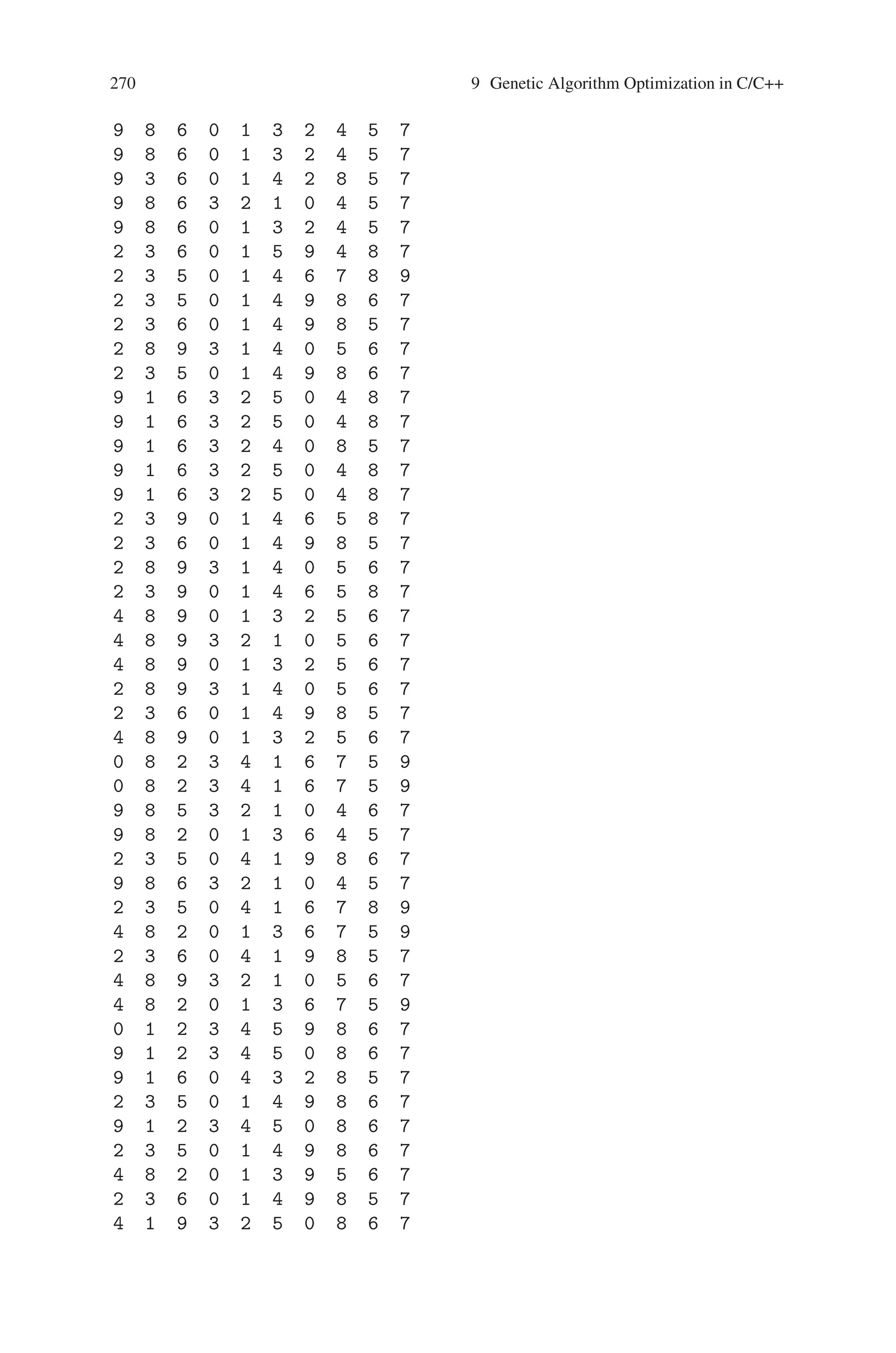
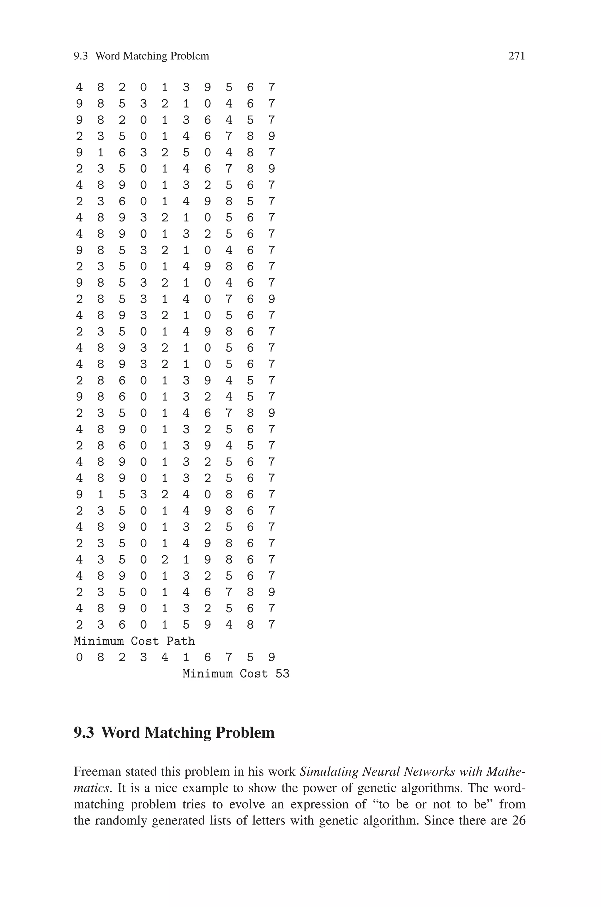
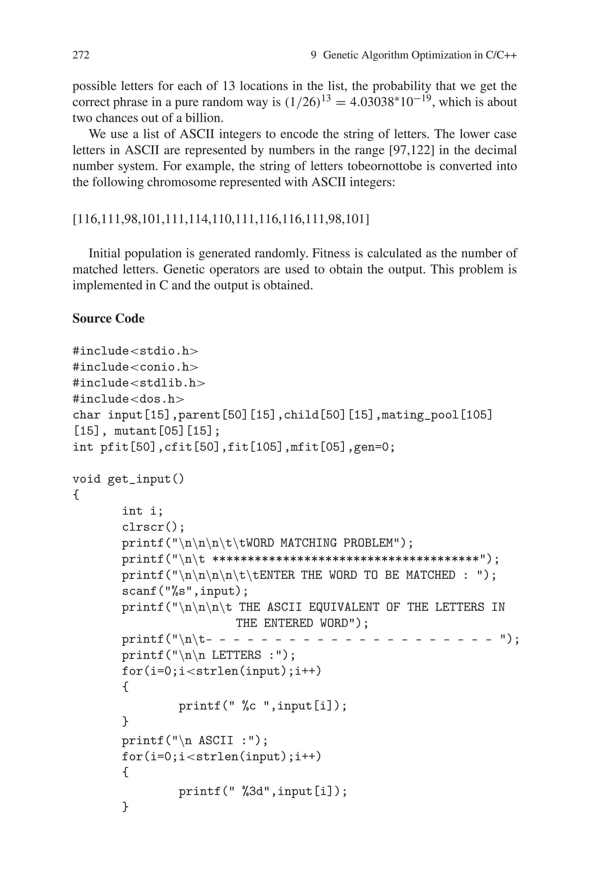
![272 9 Genetic Algorithm Optimization in C/C++
possible letters for each of 13 locations in the list, the probability that we get the
correct phrase in a pure random way is (1/26)13 = 4.03038∗10−19, which is about
two chances out of a billion.
We use a list of ASCII integers to encode the string of letters. The lower case
letters in ASCII are represented by numbers in the range [97,122] in the decimal
number system. For example, the string of letters tobeornottobe is converted into
the following chromosome represented with ASCII integers:
[116,111,98,101,111,114,110,111,116,116,111,98,101]
Initial population is generated randomly. Fitness is calculated as the number of
matched letters. Genetic operators are used to obtain the output. This problem is
implemented in C and the output is obtained.
Source Code
#includestdio.h
#includeconio.h
#includestdlib.h
#includedos.h
char input[15],parent[50][15],child[50][15],mating_pool[105]
[15], mutant[05][15];
int pfit[50],cfit[50],fit[105],mfit[05],gen=0;
void get_input()
{
int i;
clrscr();
printf(nnnttWORD MATCHING PROBLEM);
printf(nt **************************************);
printf(nnnnttENTER THE WORD TO BE MATCHED : );
scanf(%s,input);
printf(nnnt THE ASCII EQUIVALENT OF THE LETTERS IN
THE ENTERED WORD);
printf(nt- - - - - - - - - - - - - - - - - - - - - );
printf(nn LETTERS :);
for(i=0;istrlen(input);i++)
{
printf( %c ,input[i]);
}
printf(n ASCII :);
for(i=0;istrlen(input);i++)
{
printf( %3d,input[i]);
}](https://image.slidesharecdn.com/s-220425101513/75/S-N-Sivanandam-S-N-Deepa-Introduction-to-Genetic-Algorithms-2008-ISBN-3540731894-pdf-284-2048.jpg)
![9.3 Word Matching Problem 273
getch();
}
void initial_pop()
{
int i,j;
randomize();
for(i=0;i50;i++)
{
for(j=0;jstrlen(input);j++)
{
parent[i][j]=random(26)+97;
if(parent[i][j]==input[j])
{
pfit[i]++;
}
}
}
}
void display()
{
int i,j,nexti;
clrscr();
printf(nntt THE CHROMOSOMES OF PARENTS
AND CHILDREN);
printf(nt - - - - - - - - - - - - - - - - - - -n);
printf(ntt PREVIOUS GENERATION CHILDREN
CHROMOSOMESnn);
for(i=0;i50;i++)
{
if(((i)%4)==0) printf(n);
for(j=0;jstrlen(input);j++)
{
printf(%c,child[i][j]);
}
printf(% 2d ,cfit[i]);
}
printf(ntttMUTANTS OF THIS GENERATIONn);
for(i=0;i05;i++)
{
if (i==3) printf(n);
for(j=0;jstrlen(input);j++)
{
printf(%c,mutant[i][j]);
}
printf(% 2d ,mfit[i]);
}](https://image.slidesharecdn.com/s-220425101513/75/S-N-Sivanandam-S-N-Deepa-Introduction-to-Genetic-Algorithms-2008-ISBN-3540731894-pdf-285-2048.jpg)
![274 9 Genetic Algorithm Optimization in C/C++
getch();
clrscr();
printf(nntt THE CHROMOSOMES OF PARENTS AND
CHILDREN);
printf(nt - - - - - - - - - - - - - - - -n);
printf(ntt NEXT GENERATION PARENTS
CHROMOSOMESnn);
for(i=0;i50;i++)
{
if(((i)%4)==0) printf(n);
for(j=0;jstrlen(input);j++)
{
printf(%c,parent[i][j]);
}
printf(% 2d ,pfit[i]);
}
getch();
}
void reproduction() //sorting_based_on_fitness()
{
char tempc;
int temp;
int i,j,k;
for(i=0;i50;i++)
{
for(j=0;jstrlen(input);j++)
{
mating_pool[i][j]=parent[i][j];
fit[i]=pfit[i];
}
}
for(i=50;i100;i++)
{
for(j=0;jstrlen(input);j++)
{
mating_pool[i][j]=child[i-50][j];
fit[i]=cfit[i-50];
}
}
for(i=100;i105;i++)
{
for(j=0;jstrlen(input);j++)
{
mating_pool[i][j]=mutant[i-100][j];
fit[i]=mfit[i-100];
}](https://image.slidesharecdn.com/s-220425101513/75/S-N-Sivanandam-S-N-Deepa-Introduction-to-Genetic-Algorithms-2008-ISBN-3540731894-pdf-286-2048.jpg)
![9.3 Word Matching Problem 275
}
//sorting
for(i=0;i105;i++)
{
for(j=i+1;j105;j++)
{
if(fit[i]fit[j])
{
for(k=0;kstrlen(input);k++)
{
tempc=mating_pool[i][k];
mating_pool[i][k]=
mating_pool[j][k];
mating_pool[j][k]=tempc;
temp=fit[i];
fit[i]=fit[j];
fit[j]=temp;
}
}
}
}
for(i=0;i50;i++)
{
for(j=0;jstrlen(input);j++)
{
parent[i][j]=mating_pool[i][j];
pfit[i]=fit[i];
}
}
for(i=50;i100;i++)
{
for(j=0;jstrlen(input);j++)
{
child[i-50][j]=mating_pool[i][j];
cfit[i-50]=fit[i];
}
}
}
void crossover()
{
int xover_pt;
int i,j,k;
for(i=0;i50;i++)
{
xover_pt=random(strlen(input));](https://image.slidesharecdn.com/s-220425101513/75/S-N-Sivanandam-S-N-Deepa-Introduction-to-Genetic-Algorithms-2008-ISBN-3540731894-pdf-287-2048.jpg)
![276 9 Genetic Algorithm Optimization in C/C++
cfit[i]=0;
cfit[i+1]=0;
for(j=0;jxover_pt;j++)
{
child[i][j]=parent[i][j];
if (input[j]==child[i][j])
cfit[i]++;
child[i+1][j]=parent[i+1][j];
if(input[j]==child[i+1][j])
cfit[i+1]++;
}
for(j=xover_pt;jstrlen(input);j++)
{
child[i][j]=parent[i+1][j];
if(input[j]==child[i][j])
cfit[i]++;
child[i+1][j]=parent[i][j];
if(input[j]==child[i+1][j])
cfit[i+1]++;
}
i++;
}
}
void mutation()
{
int i,mut_pt,j;
char mut_val;
randomize();
for(i=0;i05;i++)
{
mut_pt=random(strlen(input));
mut_val=random(26)+97;
mfit[i]=0;
for(j=0;jmut_pt;j++)
{
mutant[i][j]=parent[1][j];
if (mutant[i][j]==input[j])
{
mfit[i]++;
}
}
mutant[i][mut_pt]=mut_val;
if (mutant[i][j]==input[j])
{
mfit[i]++;](https://image.slidesharecdn.com/s-220425101513/75/S-N-Sivanandam-S-N-Deepa-Introduction-to-Genetic-Algorithms-2008-ISBN-3540731894-pdf-288-2048.jpg)
![9.3 Word Matching Problem 277
}
for(j=mut_pt+1;jstrlen(input);j++)
{
mutant[i][j]=parent[1][j];
if (mutant[i][j]==input[j])
{
mfit[i]++;
}
}
}
}
void results()
{
int i;
clrscr();
printf(nnnttWORD MATCHING PROBLEM );
printf(nt ****************************************);
printf(nnntt THE MATCHING WORD FOR THE
GIEN INPUT WORD);
printf(nntt OBTAINED USING GENETIC ALGORITHM);
printf(nnttt );
for(i=0;istrlen(input);i++)
{
printf(%c,parent[0][i]);
}
printf(nttt –);
for(i=0;istrlen(input);i++)
{
printf(-);
}
printf(–nnntt USER INPUT : %s,input);
printf(nnnt THE FITNESS OF THE GA GENERATED WORD
AND THE USER’S INPUT);
printf(nntttt %2d/%d,pfit[0],strlen(input));
printf(nnnttt GENERATIONS COUNT : %d,gen);
}
int input_choice()
{
int choice,i;
clrscr();
printf(nnnnttt GENEREATION NUMBER : %d,gen);
printf(ntt –––––––––––––––);
printf(nnnttTHE FITTEST INDIVIDUAL TILL THE PREVIOUS
GENERATIONnnntttt);
for(i=0;istrlen(input);i++)](https://image.slidesharecdn.com/s-220425101513/75/S-N-Sivanandam-S-N-Deepa-Introduction-to-Genetic-Algorithms-2008-ISBN-3540731894-pdf-289-2048.jpg)
![278 9 Genetic Algorithm Optimization in C/C++
{
printf(%c,parent[0][i]);
}
printf( / );
for(i=0;istrlen(input);i++)
{
printf(%c,input[i]);
}
printf(nnnttt WITH A FITNESS OF %d/%d,pfit[0],
strlen(input));
printf(nnnnttENTER YOUR CHOICE (TO CONTINUE 1 TO
EXIT 0) : );
scanf(%d,choice);
return choice;
}
void main()
{
int i,choice;
clrscr();
get_input();
initial_pop();
//display();
reproduction(); //sorting_based_on_fitness();
display();
printf(nENTER YOUR CHOICE (TO CONTINUE 1 TO
EXIT 0) : );
scanf(%d,choice);
while((choice==1)(pfit[0]!=strlen(input)))
{
crossover();
gen++;
mutation();
reproduction(); //sorting_based_on_fitness();
display();
choice=input_choice();
}
sound(1000);
delay(200);
nosound();
delay(200);
results();
getch();
sound(1000);
delay(200);
nosound();
}](https://image.slidesharecdn.com/s-220425101513/75/S-N-Sivanandam-S-N-Deepa-Introduction-to-Genetic-Algorithms-2008-ISBN-3540731894-pdf-290-2048.jpg)
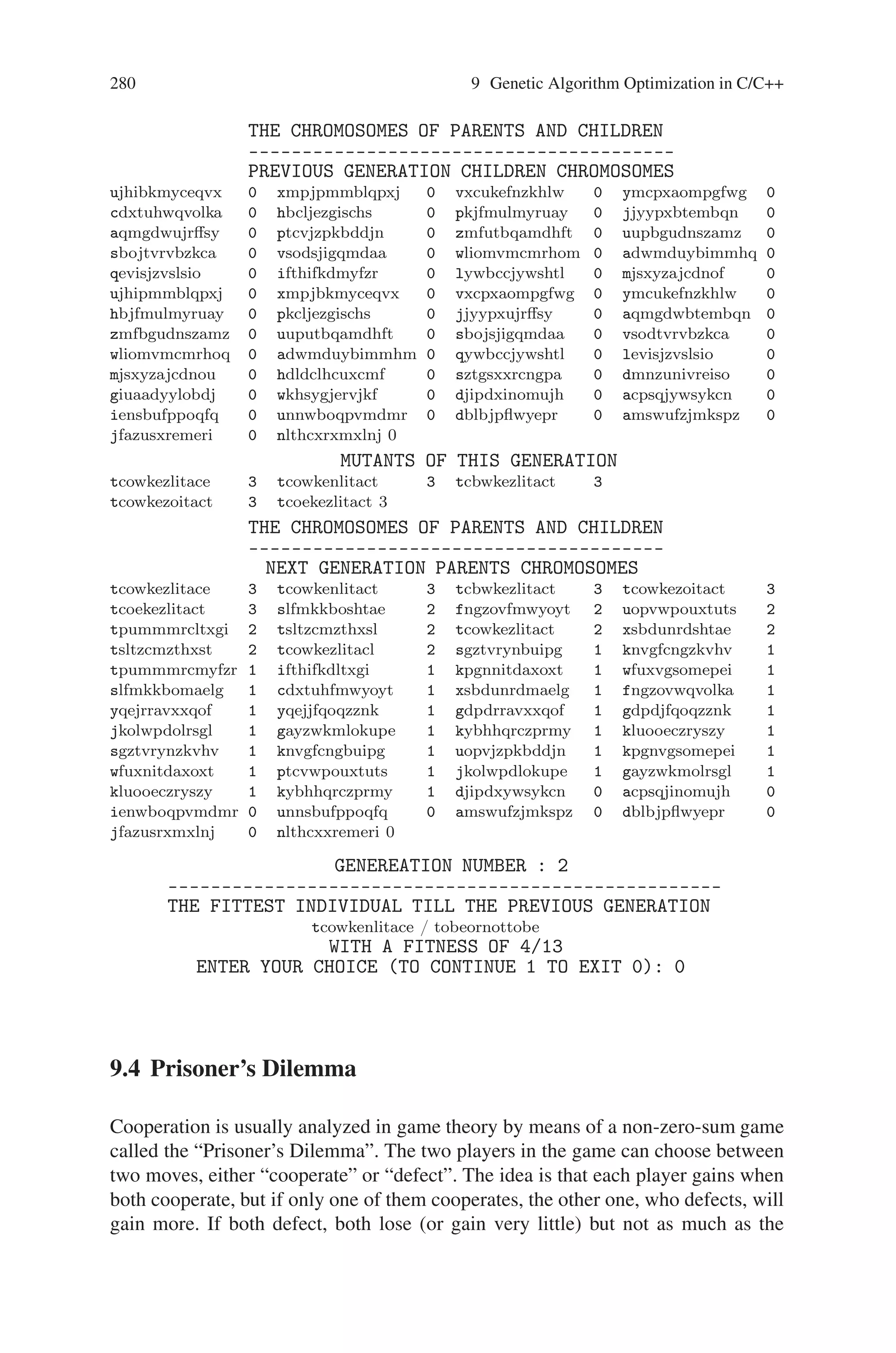
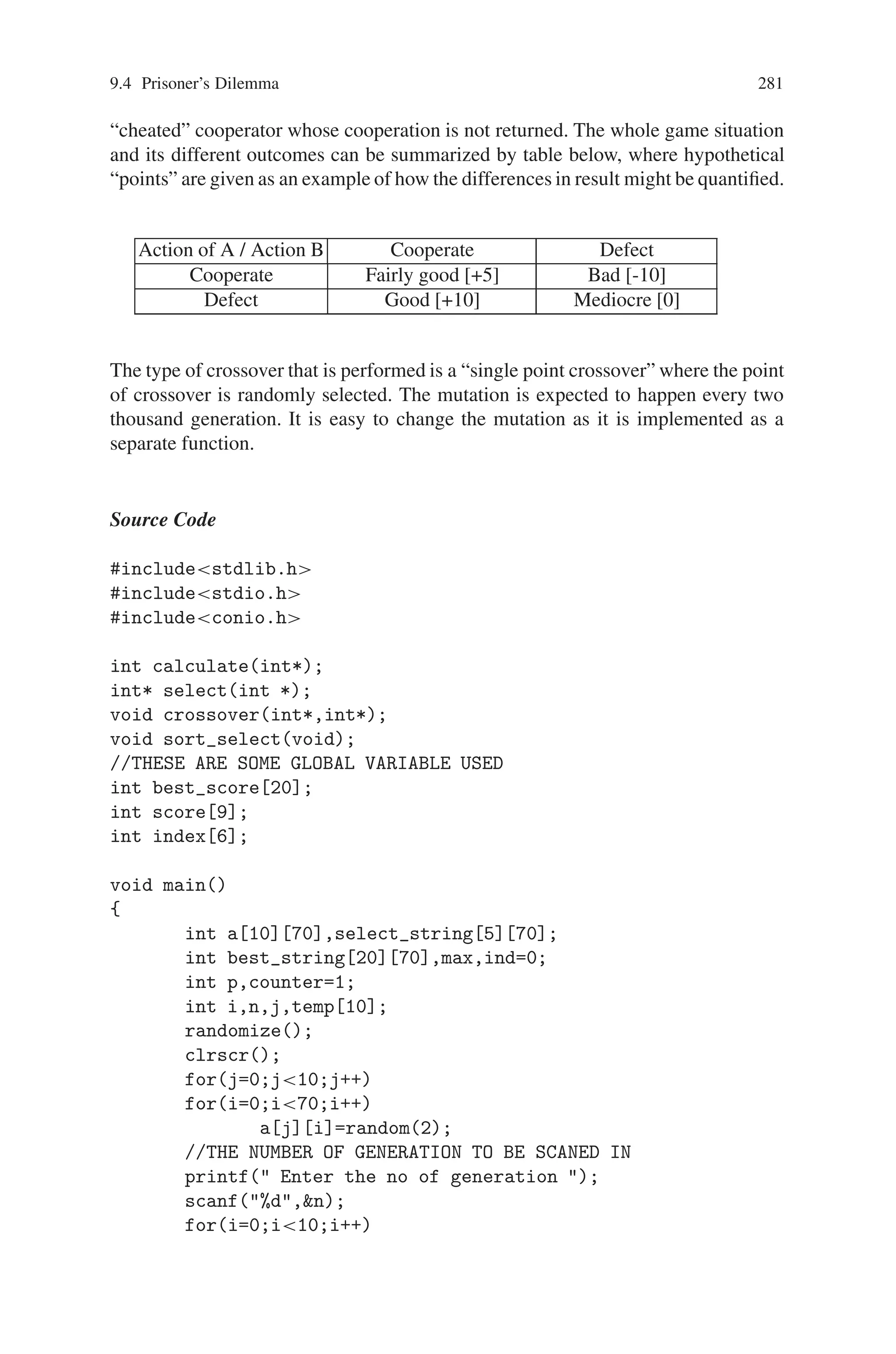
![9.4 Prisoner’s Dilemma 281
“cheated” cooperator whose cooperation is not returned. The whole game situation
and its different outcomes can be summarized by table below, where hypothetical
“points” are given as an example of how the differences in result might be quantified.
Action of A / Action B Cooperate Defect
Cooperate Fairly good [+5] Bad [-10]
Defect Good [+10] Mediocre [0]
The type of crossover that is performed is a “single point crossover” where the point
of crossover is randomly selected. The mutation is expected to happen every two
thousand generation. It is easy to change the mutation as it is implemented as a
separate function.
Source Code
#includestdlib.h
#includestdio.h
#includeconio.h
int calculate(int*);
int* select(int *);
void crossover(int*,int*);
void sort_select(void);
//THESE ARE SOME GLOBAL VARIABLE USED
int best_score[20];
int score[9];
int index[6];
void main()
{
int a[10][70],select_string[5][70];
int best_string[20][70],max,ind=0;
int p,counter=1;
int i,n,j,temp[10];
randomize();
clrscr();
for(j=0;j10;j++)
for(i=0;i70;i++)
a[j][i]=random(2);
//THE NUMBER OF GENERATION TO BE SCANED IN
printf( Enter the no of generation );
scanf(%d,n);
for(i=0;i10;i++)](https://image.slidesharecdn.com/s-220425101513/75/S-N-Sivanandam-S-N-Deepa-Introduction-to-Genetic-Algorithms-2008-ISBN-3540731894-pdf-293-2048.jpg)
![282 9 Genetic Algorithm Optimization in C/C++
score[i]=calculate(a[i][0]);
//function for sorting the score array and finding the index
of best score
sort_select();
for(i=0;i7;i++)
{
p=index[i]; //THE ORDER OF BEST SCORE STORED IN
INDEX.
for(j=0;j70;j++)
select_string[i][j]=a[p][j];
}
best_score[0]=score[0];
for(i=0;i70;i++)
best_string[0][i]=select_string[0][i];
while(counter n)
{
for(i=0;i7;i=i+2)
crossover(a[i][0],a[i+1][0]);
for(i=0;i9;i++)
score[i]=0;
for(i=0;i7;i++)
score[i]=calculate(a[i][0]);
//CALCULATE FUNCTION RETURNS SCORE OF EACH STRING
sort_select();
best_score[counter]=score[0];
p=index[0];
for(j=0;j70;j++)
best_string[counter][j]=a[p][j];
counter++;
}
//OUTPUT THE BEST SCORES.
for(p=0;pn;p++)
{
printf(The best score in the generation
%d :,p+1);
printf( %d n, best_score[p]);
}
//OUTPUT THE BEST STRINGS.
for(i=0;in;i++)
{
printf(nnTHE BEST STRNG IN GENERATION %d
:nn, i+1);
for(j=0;j70;j++)
{](https://image.slidesharecdn.com/s-220425101513/75/S-N-Sivanandam-S-N-Deepa-Introduction-to-Genetic-Algorithms-2008-ISBN-3540731894-pdf-294-2048.jpg)
![9.4 Prisoner’s Dilemma 283
if(j%2==0j!=0)
printf( );
if(best_string[i][j] ==1)
printf(d);
//COVERTING 1’S AND 0’S TO d AND c
else
printf(c);
}
}
//CALCULATING THE BEST OF THE BEST
for(i=0;in;i++)
temp[i]=best_score[i];
max=temp[0];
for(i=1;in;i++)
{
if(maxtemp[i])
{
max=temp[i];
ind=i;
}
}
//CALCULATING THE BEST FROM THE SELECTED.
printf(nn);
printf(nTHE BEST STRING IN ALL GENERATION IS nn);
for(i=0;i70;i++)
{
if(i%2==0i!=0)
printf( );
if(best_string[ind][i]==1)
printf(d);
else
printf(c);
}
printf(nnTHE CORRESPONDING BEST SCORE IS: %d ,best
_score[ind]);
getch();
}
int calculate(int* ptr)
{
int *a;
int p1,p2,i;
a=ptr;
p1=0; p2=0;](https://image.slidesharecdn.com/s-220425101513/75/S-N-Sivanandam-S-N-Deepa-Introduction-to-Genetic-Algorithms-2008-ISBN-3540731894-pdf-295-2048.jpg)
![284 9 Genetic Algorithm Optimization in C/C++
for(i=0;i70;i=i+2) //calculating the values according
to truth table.
{
if(a[i]==1 a[i+1]==1)
{
p1=p1+3; p2=p2+3;
}
if(a[i]==1 a[i+1]==0)
{
p1=p1+5; p2=p2+0;
}
if(a[i]==0 a[i+1]==1)
{
p1=p1+0; p2=p2+5;
}
if(a[i]==0 a[i+1]==0)
{
p1=p1+1; p2=p2+1;
}
}
return(p1+p2); //RETRUN THE TOTAL SCORE OF THE STRING.
}
void sort_select() //ORDINARY SORTING PROCEDURE
{
int temp[9],i,j,t;
for(i=0;i10;i++)
temp[i]=score[i];
for(i=0;i10;i++)
for(j=9;j=i;j–)
{
if(temp[i]temp[j]) //USUSAL SWAPPING
PROCEDURE.
{
t=temp[j];
temp[j]=temp[i];
temp[i]=t;
}
}
for(i=0;i7;i++)
for(j=0;j10;j++)
if(temp[i]==score[j])
index[i]=j;
score[0]=temp[0];](https://image.slidesharecdn.com/s-220425101513/75/S-N-Sivanandam-S-N-Deepa-Introduction-to-Genetic-Algorithms-2008-ISBN-3540731894-pdf-296-2048.jpg)
![9.4 Prisoner’s Dilemma 285
}
void crossover(int *ptr1,int *ptr2)
{
int temp,i,j;
int ind=random(60); //RANDOM POINT OF CROSSOVER
for(i=ind;i70;i++)
{
temp=ptr1[i];
ptr1[i]=ptr2[i];
ptr2[i]=temp;
}
}
Output
Enter the no of generation 5
The best score in the generation 1: 171
The best score in the generation 2: 160
The best score in the generation 3: 170
The best score in the generation 4: 166
The best score in the generation 5: 169
The best string in generation 1:
dd dc cd dc dc cd cd dd cc dc dc dc dd dc dd cd dc cd
cd cc dc cd cc cd dd cd cd dd cd dc cc cd dc dd dd
The best string in generation 2:
cd cc cd cc cd cd dd dc cd cc dc cc dd cd dd dd cc cc dc dd
dc cd cd dd dc dd dd cc cd dd dc dc cd dc cc
The best string in generation 3:
cd cc cd cc cd cd dc dd cd dc dd cc cd cd cc dd cd dd dc cd
dc dc dd cd dc dc dc cd cd cd dc dc dd dc dd
The best string in generation 4:
cd cc cd cc cd cd dc dd cd dc dd cc cd cd cc dd cd dd dc cd
dc dc dd dd dc dd dd cc cd dd dc dc cd dc cc
The best string in generation 5:
Cd dd cc cd dd dc cd cc dd cd dd dd dc cd cd cc dc cd cd dc
cc dd dd dc dc dc dd dc dc cd dc cc dc cd dd](https://image.slidesharecdn.com/s-220425101513/75/S-N-Sivanandam-S-N-Deepa-Introduction-to-Genetic-Algorithms-2008-ISBN-3540731894-pdf-297-2048.jpg)
![286 9 Genetic Algorithm Optimization in C/C++
The best string in all generation is
dd dc cd dc dc cd cd dd cc dc dc dc dd dc dd cd dc
cd cd cc dc cd cc cd dd cd cd dd cd dc cc cd dc dd dd
The corresponding best score is : 171
9.5 Maximize f(x) = x2
A C++ Program for maximizing f(x) = x2 using genetic algorithm, where x is
ranges from 0 to 31.
1. Generate Initial four populations of binary string with 5 bits length.
2. Calculate corresponding x and fitness value f(x) = x2.
3. Use the tournament selection method to generate new four populations.
4. Apply cross-over operator to the new four populations and generate new popula-
tions.
5. Apply mutation operator for each population.
6. Repeat the step 2 to 5 for some 20 iterations.
7. Finally print the result.
Source Code
#includestdio.h
#includeiostream.h
#includeconio.h
#includestdlib.h
#includemath.h
#includetime.h
int pop[10][10],npop[10][10],tpop[10][10],x[10],fx[10],m_max=1,
ico=0,ico1,it=0;
void iter(int [10][10],int,int);
int u_rand(int);
void tour_sel(int,int);
void cross_ov(int,int);
void mutat(int,int);
void main()
{
int k,m,j,i,p[10],n=0,a[10],nit;
//time_t t;
clrscr();
//srand((unsigned) time(t));](https://image.slidesharecdn.com/s-220425101513/75/S-N-Sivanandam-S-N-Deepa-Introduction-to-Genetic-Algorithms-2008-ISBN-3540731894-pdf-298-2048.jpg)
![9.5 Maximize f(x) = x2 287
randomize();
/*while (n4)
{
k=0;
p[n]=u_rand(32);
a[n]=p[n];
for(i=0;i=n;i++)
{
if (p[n]==p[i] n!=i)
k++;
}
if (k==0)
{
n++;
}
} */
coutEnter the number of Population in each iteration is : ;
cinn;
coutEnter the number of iteration is : ;
cinnit;
m=5;
for(i=0;in;i++)
{
for(j=m-1;j=0;j–)
{
/*if (a[i]==0)
pop[i][j]=0;
else
{*/
pop[i][j]=u_rand(2);
// a[i]=a[i]/2;
// }
}
}
coutnIteration it is :n;
iter(pop,n,m);
it++;
getch();
do
{
it++;
coutnIteration it is :n;
tour_sel(n,m);
iter(pop,n,m);
getch();](https://image.slidesharecdn.com/s-220425101513/75/S-N-Sivanandam-S-N-Deepa-Introduction-to-Genetic-Algorithms-2008-ISBN-3540731894-pdf-299-2048.jpg)
![288 9 Genetic Algorithm Optimization in C/C++
}while(itnit);
coutnnAfter the ico1 Iteration, the Maximum Value
is : (int)
sqrt(m_max);
getch();
}
void iter(int pp[10][10],int o, int p)
{
int i,j,sum,avg,max=1;
for(i=0;io;i++)
{
x[i]=0;
for(j=0;jp;j++)
{
x[i]=x[i]+(pp[i][j]*pow(2,p-1-j));
}
fx[i]=x[i]*x[i];
sum=sum+fx[i];
if (max=fx[i])
max=fx[i];
}
avg=sum/o;
coutnnS.No.tPopulationtXtf(X)nn;
for(i=0;io;i++)
{
couticot;
ico++;
for(j=0;jp;j++)
coutpp[i][j];
coutttx[i]tfx[i]n;
}
coutnt Sum : sumtAverage : avgtMaximum :
maxn;
if (m_maxmax)
{
m_max=max;
ico1=it;
}
}
int u_rand(int x)
{
int y;
y=rand()%x;
return(y);
}](https://image.slidesharecdn.com/s-220425101513/75/S-N-Sivanandam-S-N-Deepa-Introduction-to-Genetic-Algorithms-2008-ISBN-3540731894-pdf-300-2048.jpg)
![9.5 Maximize f(x) = x2 289
void tour_sel(int np,int mb)
{
int i,j,k,l,co=0,cc;
//time_t t;
//srand((unsigned) time(t));
do
{
k=u_rand(np);
do
{
cc=0;
l=u_rand(np);
if (k==l)
cc++;
}while(cc!=0);
if (fx[k]fx[l])
{
for(j=0;jmb;j++)
npop[co][j]=pop[k][j];
}
else if (fx[k]fx[l])
{
for(j=0;jmb;j++)
npop[co][j]=pop[l][j];
}
co++;
}while(conp);
getch();
cross_ov(np,mb);
getch();
}
void cross_ov(int np1,int mb1)
{
int i,j,k,l,co,temp;
//time_t t;
//srand((unsigned) time(t));
i=0;
do
{
k=rand()%2;
do
{](https://image.slidesharecdn.com/s-220425101513/75/S-N-Sivanandam-S-N-Deepa-Introduction-to-Genetic-Algorithms-2008-ISBN-3540731894-pdf-301-2048.jpg)
![290 9 Genetic Algorithm Optimization in C/C++
co=0;
l=u_rand(mb1);
if (((k==0) (l==0)) || ((k==1) (l==mb1)))
co++;
}while(co!=0);
if ((k==0) (l!=0))
{
for(j=0;jl;j++)
{
temp=npop[i][j];
npop[i][j]=npop[i+1][j];
npop[i+1][j]=temp;
}
}
else if ((k==1) (l!=mb1))
{
for(j=l;jmb1;j++)
{
temp=npop[i][j];
npop[i][j]=npop[i+1][j];
npop[i+1][j]=temp;
}
}
i=i+2;
}while(inp1);
for(i=0;inp1;i++)
{
for(j=0;jmb1;j++)
{
tpop[i][j]=npop[i][j];
//pop[i][j]=tpop[i][j];
}
}
mutat(np1,mb1);
}
void mutat(int np2,int mb2)
{
int i,j,r,temp,k,z;
i=0;
do
{
for(k=0;knp2;k++)](https://image.slidesharecdn.com/s-220425101513/75/S-N-Sivanandam-S-N-Deepa-Introduction-to-Genetic-Algorithms-2008-ISBN-3540731894-pdf-302-2048.jpg)
![9.5 Maximize f(x) = x2 291
{
r=0;
if (i!=k)
{
for(j=0;jmb2;j++)
{
if (tpop[i][j]==tpop[k][j])
r++;
}
if (r!=mb2-1)
{
z=u_rand(mb2);
if (tpop[i][z]==0)
tpop[i][z]=1;
else
tpop[i][z]=0;
if (npop[k][u_rand(mb2)]==0)
npop[k][u_rand(mb2)]=1;
else
npop[k][u_rand(mb2)]=0;
mutat(k,mb2);
}
}
}
i++;
}while(inp2);
for(i=0;inp2;i++)
{
for(j=0;jmb2;j++)
{
pop[i][j]=tpop[i][j];
}
}
}
Output
Enter the number of Population in each iteration is : 4
Enter the number of iteration is : 5
Iteration 0 is :
S.No. Population X f(X)
0 01001 9 81
1 01110 14 196
2 11101 29 841
3 01111 15 225
Sum : 1620 Average : 405 Maximum : 841](https://image.slidesharecdn.com/s-220425101513/75/S-N-Sivanandam-S-N-Deepa-Introduction-to-Genetic-Algorithms-2008-ISBN-3540731894-pdf-303-2048.jpg)
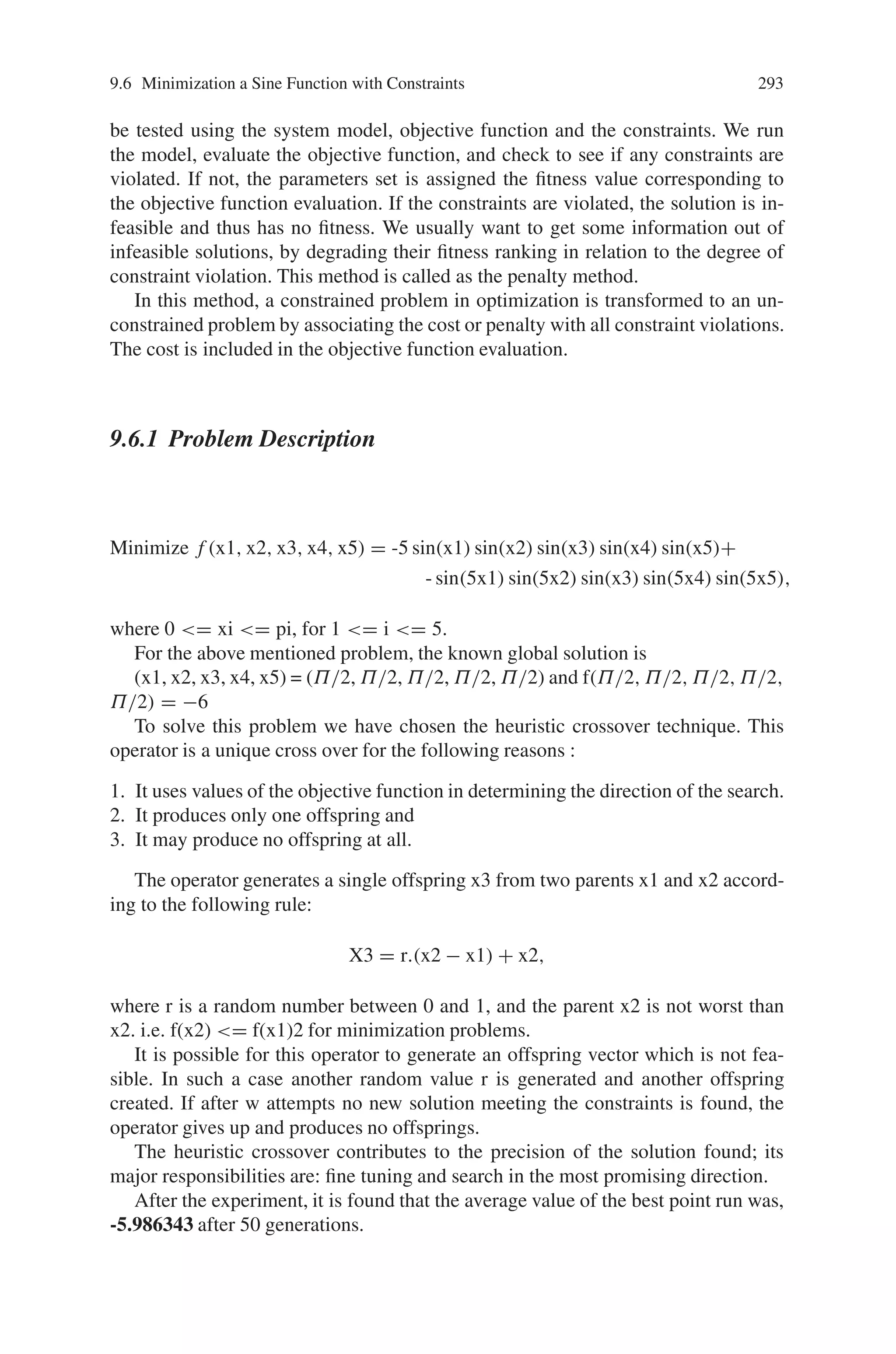
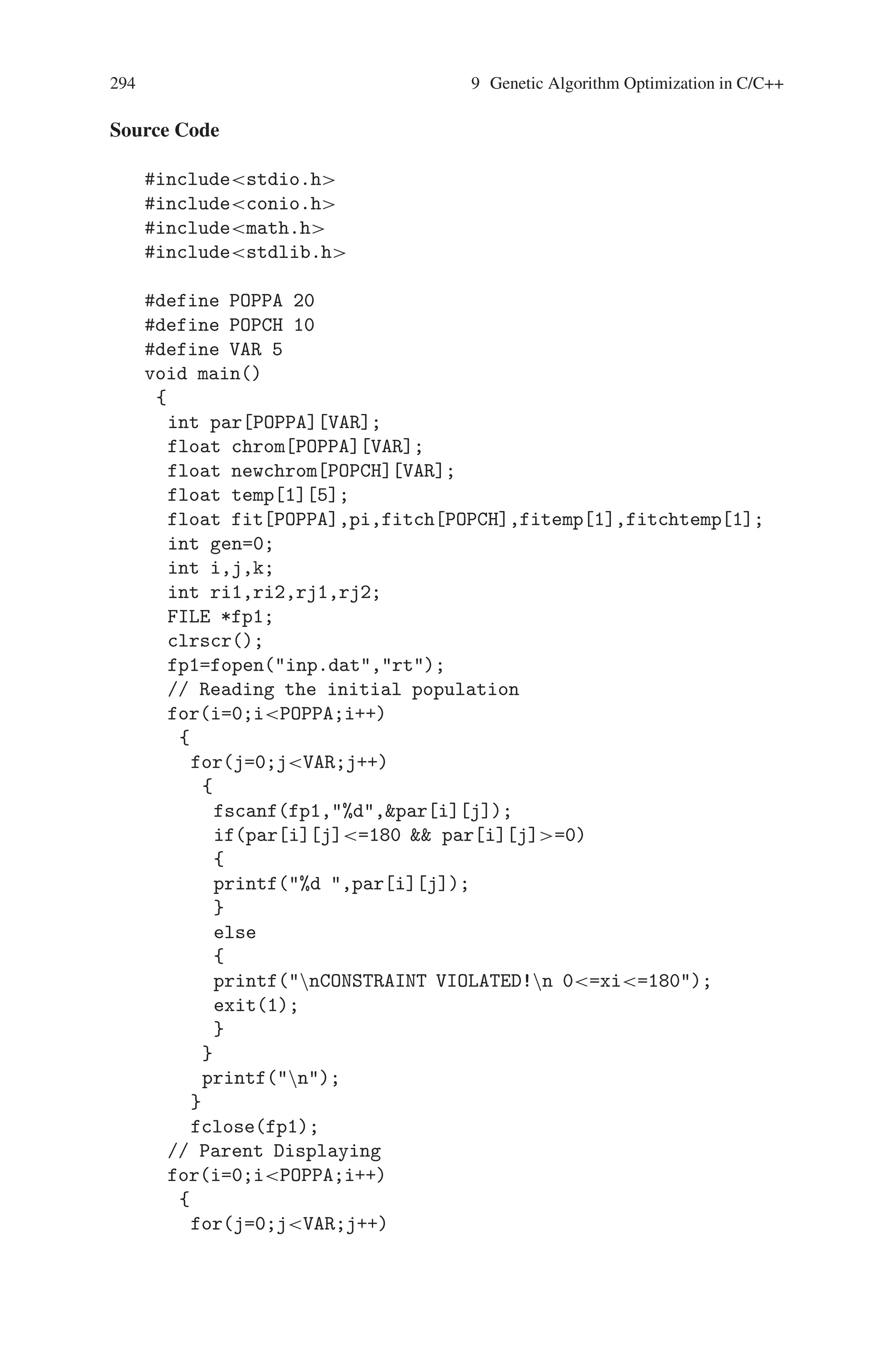
![294 9 Genetic Algorithm Optimization in C/C++
Source Code
#includestdio.h
#includeconio.h
#includemath.h
#includestdlib.h
#define POPPA 20
#define POPCH 10
#define VAR 5
void main()
{
int par[POPPA][VAR];
float chrom[POPPA][VAR];
float newchrom[POPCH][VAR];
float temp[1][5];
float fit[POPPA],pi,fitch[POPCH],fitemp[1],fitchtemp[1];
int gen=0;
int i,j,k;
int ri1,ri2,rj1,rj2;
FILE *fp1;
clrscr();
fp1=fopen(inp.dat,rt);
// Reading the initial population
for(i=0;iPOPPA;i++)
{
for(j=0;jVAR;j++)
{
fscanf(fp1,%d,par[i][j]);
if(par[i][j]=180 par[i][j]=0)
{
printf(%d ,par[i][j]);
}
else
{
printf(nCONSTRAINT VIOLATED!n 0=xi=180);
exit(1);
}
}
printf(n);
}
fclose(fp1);
// Parent Displaying
for(i=0;iPOPPA;i++)
{
for(j=0;jVAR;j++)](https://image.slidesharecdn.com/s-220425101513/75/S-N-Sivanandam-S-N-Deepa-Introduction-to-Genetic-Algorithms-2008-ISBN-3540731894-pdf-306-2048.jpg)
![9.6 Minimization a Sine Function with Constraints 295
{
chrom[i][j]=(float)par[i][j];
printf(%f ,chrom[i][j]);
}
printf(n);
}
pi = 4.0*atan(1.0);
clrscr();
while(gen!=50)
{
printf(Next Generation: %dn,gen);
for(i=0;iPOPPA;i++)
{
fit[i]=-
5*(sin(pi*chrom[i][0]/180))*sin(pi*chrom[i][1]/180)
*sin(pi*chrom[i][2]/180)
*sin(pi*chrom[i][3]/180)*sin(pi*chrom[i][4]/180)-
sin(5*pi*chrom[i][0]/180)*sin(5*pi*chrom[i][1]/180)
*sin(5*pi*chrom[i][2]/180)
*sin(5*pi*chrom[i][3]/180)*sin(5*pi*
chrom[i][4]/180);
printf(%f %f %f %f %f %fn,chrom[i][0],chrom[i][1],
chrom[i][2],chrom[i][3],chrom[i][4],fit[i]);
}
printf(n);
//Crossover
for(i=0,k=10;iPOPCH;i++,k++)
{
for(j=0;jVAR;j++)
{
if(chrom[i][j]=chrom[k][j])
newchrom[i][j]=((random(10)/10)*(chrom[k][j]-chrom[i][j]))
+chrom[k][j];
else
newchrom[i][j]=((random(10)/10)*(chrom[i][j]-chrom[k][j]))
+chrom[i][j];
}
}
//calculate fitness for children
printf(child fitness:n);
for(i=0;iPOPCH;i++)
{
fitch[i]=-
5*(sin(pi*newchrom[i][0]/180))*sin(pi*newchrom[i][1]/180)
*sin(pi*newchrom[i][2]/180)*sin(pi*newchrom[i][3]/180)](https://image.slidesharecdn.com/s-220425101513/75/S-N-Sivanandam-S-N-Deepa-Introduction-to-Genetic-Algorithms-2008-ISBN-3540731894-pdf-307-2048.jpg)
![296 9 Genetic Algorithm Optimization in C/C++
*sin(pi*newchrom[i][4]/180)-
sin(5*pi*newchrom[i][0]/180)*sin(5*pi*newchrom[i][1]/180)
*sin(5*pi*newchrom[i][2]/180)*sin(5*pi*newchrom[i][3]/180)
*sin(5*pi*newchrom[i][4]/180);
printf(%fn,fitch[i]);
}
printf(nnn);
//sort based on fittness
//parent
for(i=0;iPOPPA;i++)
{
for(j=i+1;jPOPPA;j++)
{
if(fit[i]fit[j])
{
for(k=0;kVAR;k++)
{
temp[0][k]=chrom[j][k];
fitemp[0]=fit[j];
}
for(k=0;kVAR;k++)
{
chrom[j][k]=chrom[i][k];
fit[j]=fit[i];
}
for(k=0;kVAR;k++)
{
chrom[i][k]=temp[0][k];
fit[i]=fitemp[0];
}
}
}
}
//child
for(i=0;iPOPCH;i++)
{
for(j=i+1;jPOPCH;j++)
{
if(fitch[i]fitch[j])
{
for(k=0;kVAR;k++)
{
temp[0][k]=newchrom[j][k];
fitchtemp[0]=fitch[j];
}
for(k=0;kVAR;k++)](https://image.slidesharecdn.com/s-220425101513/75/S-N-Sivanandam-S-N-Deepa-Introduction-to-Genetic-Algorithms-2008-ISBN-3540731894-pdf-308-2048.jpg)
![9.6 Minimization a Sine Function with Constraints 297
{
newchrom[j][k]=newchrom[i][k];
fitch[j]=fitch[i];
}
for(k=0;kVAR;k++)
{
newchrom[i][k]=temp[0][k];
fitch[i]=fitchtemp[0];
}
}
}
}
//testing
printf(n);
for(i=0;iPOPCH;i++)
{
printf(%fn,fitch[i]);
}
printf(nn);
//Selecting fittest parent
for(i=10,k=0;iPOPPA;i++,k++)
{
for(j=0;jVAR;j++)
{
chrom[i][j]=newchrom[k][j];
}
}
//Mutation
if(gen%10==0)
{
randomize();
i=random(4);
j=random(4);
randomize();
ri1=random(4);
rj1=random(4);
randomize();
ri2=random(4);
rj2=random(4);
chrom[i][j]=(chrom[ri1][rj1]+chrom[ri2][rj2])/2;
}
gen++;
}//end of while
clrscr();
printf(*************************************************n);
printf(nttt OPTIMIZATIONnn);](https://image.slidesharecdn.com/s-220425101513/75/S-N-Sivanandam-S-N-Deepa-Introduction-to-Genetic-Algorithms-2008-ISBN-3540731894-pdf-309-2048.jpg)
![298 9 Genetic Algorithm Optimization in C/C++
printf(*********************************************n);
printf(nnMinimize f(x1,x2,x3,x4,x5)=-5*sinx1*sinx2*sinx3
*sinx4*sinx5
+(-Sin(5x1)*sin(5x2)*sin(5x3)*sin(5x4)*sin(5x5))nnnn);
// Displaying the last generation
//Fitness
for(i=0;iPOPCH;i++)
{
fitch[i]=-
5*(sin(pi*chrom[i][0]/180))*sin(pi*chrom[i][1]/180)
*sin(pi*chrom[i][2]/180)*sin(pi*chrom[i][3]/180)*sin(pi*
chrom[i][4]/180)-
sin(5*pi*chrom[i][0]/180)*sin(5*pi*chrom[i][1]/180)
*sin(5*pi*chrom[i][2]/180)*sin(5*pi*chrom[i][3]/180)*si
n(5*pi*chrom[i][4]/180);
printf(%fn,fitch[i]);
}
printf(The Last Generation:n);
for(i=0;iPOPCH;i++)
{
printf(%f %f %f%f%f%fn,chrom[i][0],chrom[i][1],
chrom[i][2],chrom[i][3],chrom[i][4],fitch[i]);
}
printf(n);
printf(The Solution is : %f,fitch[0]);
getch();
}
// end of main
Output
Next Generation: 0
56.000000 89.000000 65.000000 90.000000 45.000000 -2.258168
23.000000 55.000000 120.000000 56.000000 89.000000 -0.381728
32.000000 56.000000 78.000000 51.000000 62.000000 -1.349719
98.000000 5.000000 63.000000 60.000000 90.000000 -3.193594
90.000000 80.000000 70.000000 40.000000 30.000000 -1.506204
32.000000 65.000000 98.000000 45.000000 12.000000 -0.441627
56.000000 90.000000 98.000000 23.000000 150.000000 -0.460083
100.000000 110.000000 90.000000 60.000000 51.000000 -3.020786
23.000000 45.000000 90.000000 67.000000 12.000000 -0.498938
89.000000 85.000000 90.000000 45.000000 62.000000 -3.598395
45.000000 45.000000 62.000000 21.000000 89.000000 -0.422367
12.000000 20.000000 60.000000 50.000000 40.000000 0.085765
78.000000 56.000000 89.000000 23.000000 12.000000 0.055674](https://image.slidesharecdn.com/s-220425101513/75/S-N-Sivanandam-S-N-Deepa-Introduction-to-Genetic-Algorithms-2008-ISBN-3540731894-pdf-310-2048.jpg)
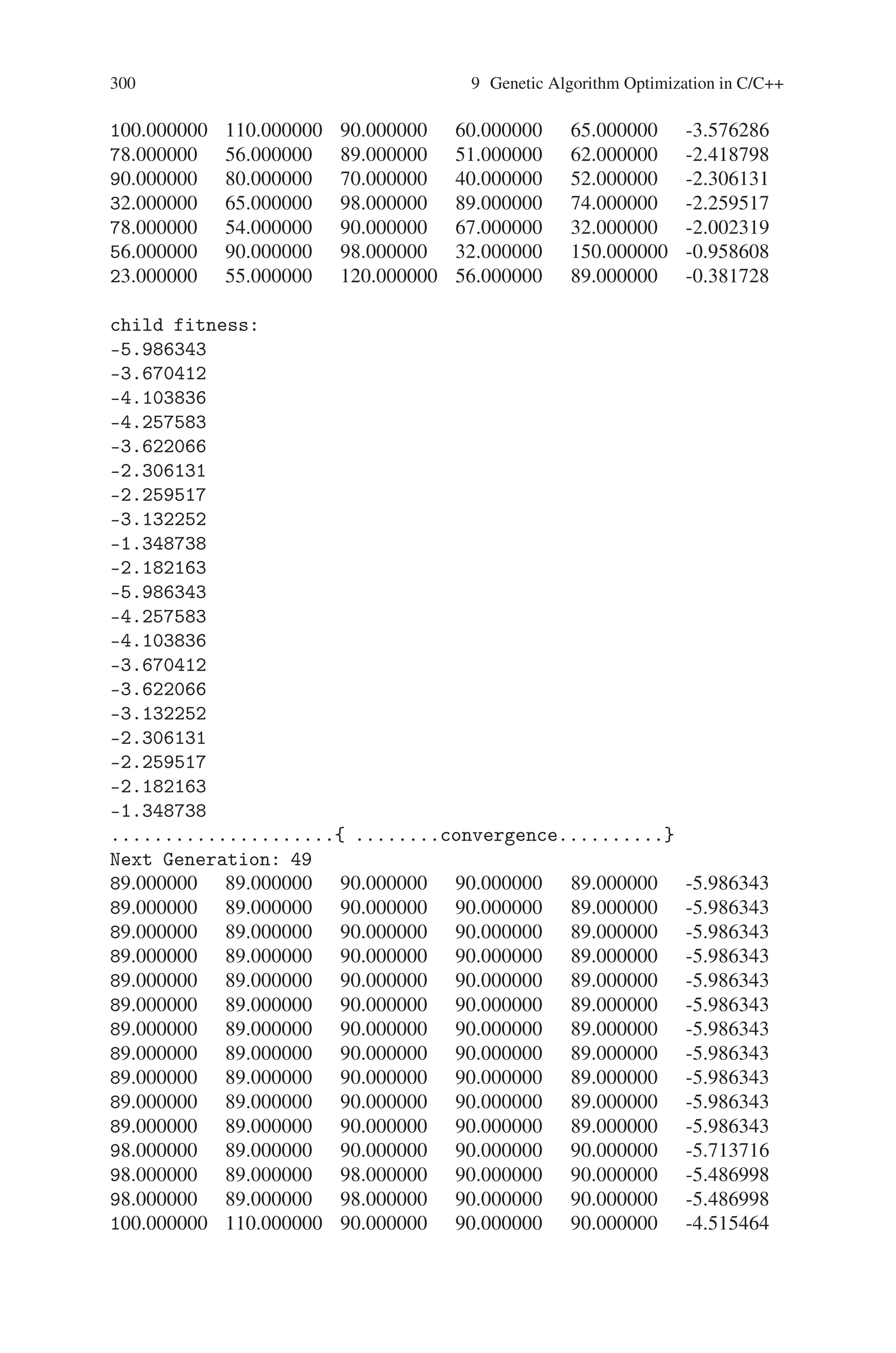
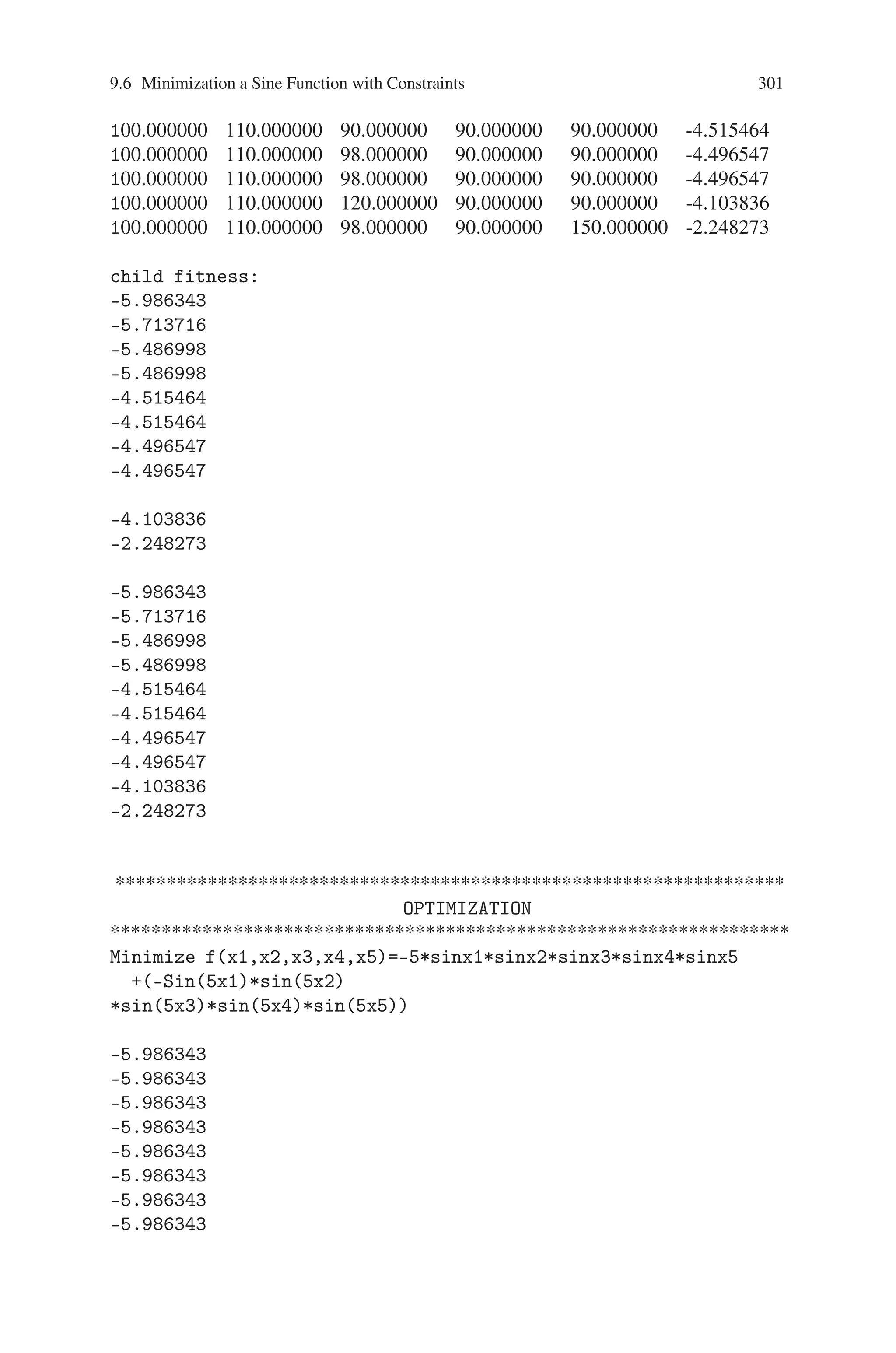
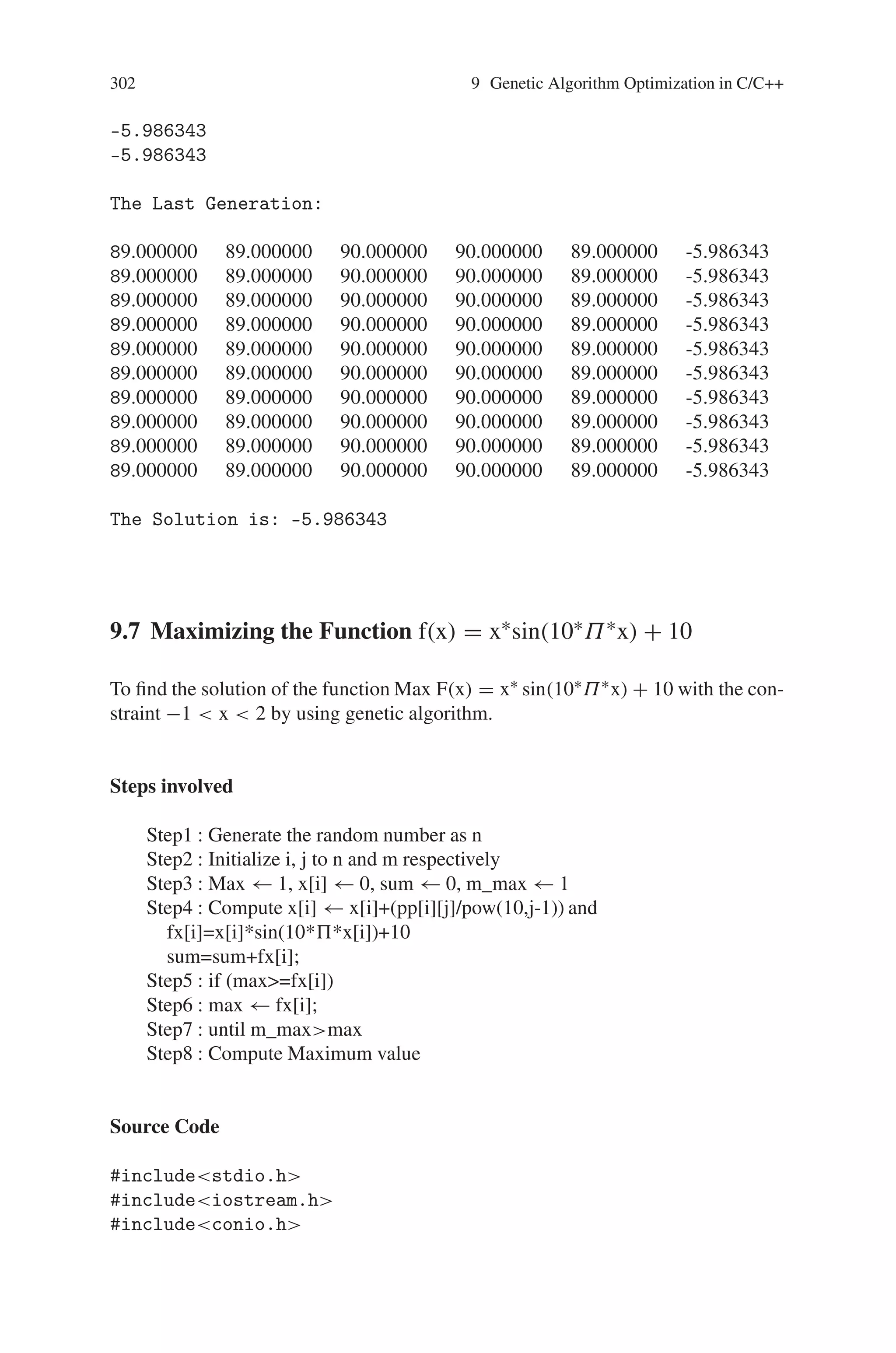
![302 9 Genetic Algorithm Optimization in C/C++
-5.986343
-5.986343
The Last Generation:
89.000000 89.000000 90.000000 90.000000 89.000000 -5.986343
89.000000 89.000000 90.000000 90.000000 89.000000 -5.986343
89.000000 89.000000 90.000000 90.000000 89.000000 -5.986343
89.000000 89.000000 90.000000 90.000000 89.000000 -5.986343
89.000000 89.000000 90.000000 90.000000 89.000000 -5.986343
89.000000 89.000000 90.000000 90.000000 89.000000 -5.986343
89.000000 89.000000 90.000000 90.000000 89.000000 -5.986343
89.000000 89.000000 90.000000 90.000000 89.000000 -5.986343
89.000000 89.000000 90.000000 90.000000 89.000000 -5.986343
89.000000 89.000000 90.000000 90.000000 89.000000 -5.986343
The Solution is: -5.986343
9.7 Maximizing the Function f(x) = x∗sin(10∗Π∗x) + 10
To find the solution of the function Max F(x) = x∗ sin(10∗Π∗x) + 10 with the con-
straint −1 x 2 by using genetic algorithm.
Steps involved
Step1 : Generate the random number as n
Step2 : Initialize i, j to n and m respectively
Step3 : Max ← 1, x[i] ← 0, sum ← 0, m_max ← 1
Step4 : Compute x[i] ← x[i]+(pp[i][j]/pow(10,j-1)) and
fx[i]=x[i]*sin(10**x[i])+10
sum=sum+fx[i];
Step5 : if (max=fx[i])
Step6 : max ← fx[i];
Step7 : until m_maxmax
Step8 : Compute Maximum value
Source Code
#includestdio.h
#includeiostream.h
#includeconio.h](https://image.slidesharecdn.com/s-220425101513/75/S-N-Sivanandam-S-N-Deepa-Introduction-to-Genetic-Algorithms-2008-ISBN-3540731894-pdf-314-2048.jpg)
![9.7 Maximizing the Function f(x) = x∗sin(10∗Π∗x) + 10 303
#includestdlib.h
#includemath.h
#includetime.h
int ico=0,ico1,it=0;
long int pop[10][10],npop[10][10],tpop[10][10];
float x[10],fx[10],m_max=1.0;
void iter(long int [10][10],int,int);
int u_rand(int);
void tour_sel(int,int);
void cross_ov(int,int);
void mutat(int,int);
void main()
{
int k,m,j,i,p[10],n=0,a[10],nit;
//time_t t;
clrscr();
//srand((unsigned) time(t));
randomize();
/*while (n4)
{
k=0;
p[n]=u_rand(32);
a[n]=p[n];
for(i=0;i=n;i++)
{
if (p[n]==p[i] n!=i)
k++;
}
if (k==0)
{
n++;
}
} */
coutEnter the number of Population in each iteration is : ;
cinn;
coutEnter the number of iteration is : ;
cinnit;
m=7;
for(i=0;in;i++)
{
for(j=0;jm;j++)
{](https://image.slidesharecdn.com/s-220425101513/75/S-N-Sivanandam-S-N-Deepa-Introduction-to-Genetic-Algorithms-2008-ISBN-3540731894-pdf-315-2048.jpg)
![304 9 Genetic Algorithm Optimization in C/C++
/*if (a[i]==0)
pop[i][j]=0;
else
{*/
if ((j==0) || (j==1))
pop[i][j]=u_rand(2);
if (j1)
pop[i][j]=u_rand(10);
// a[i]=a[i]/2;
// }
}
}
coutnIteration it is :n;
iter(pop,n,m);
it++;
getch();
do
{
it++;
coutnIteration it is :n;
tour_sel(n,m);
iter(pop,n,m);
getch();
}while(itnit);
coutnnAfter the ico1 Iteration, the Maximum Value
is :
m_max;
getch();
}
void iter(long int pp[10][10],int o, int p)
{
int i,j;
float sum,avg,max=1.0;
for(i=0;io;i++)
{
x[i]=0;
for(j=1;jp;j++)
{
if (j==1)
x[i]=x[i]+pp[i][j];
if (j1)
x[i]=x[i]+(pp[i][j]/pow(10,j-1));
}
j=0;
if (pp[i][j]==0)](https://image.slidesharecdn.com/s-220425101513/75/S-N-Sivanandam-S-N-Deepa-Introduction-to-Genetic-Algorithms-2008-ISBN-3540731894-pdf-316-2048.jpg)
![9.7 Maximizing the Function f(x) = x∗sin(10∗Π∗x) + 10 305
x[i]=-x[i];
fx[i]=x[i]*sin(10*3.14*x[i])+10;
sum=sum+fx[i];
if (max=fx[i])
max=fx[i];
}
avg=sum/o;
coutnnS.No.tPopulationtXttf(X)nn;
for(i=0;io;i++)
{
couticot;
ico++;
for(j=0;jp;j++)
coutpp[i][j];
coutttx[i]ttfx[i]n;
}
coutnt Sum : sumtAverage : avgtMaximum :
maxn;
if (m_maxmax)
{
m_max=max;
ico1=it;
}
}
int u_rand(int x)
{
int y;
y=rand()%x;
return(y);
}
void tour_sel(int np,int mb)
{
int i,j,k,l,co=0,cc;
//time_t t;
//srand((unsigned) time(t));
do
{
k=u_rand(np);
do
{
cc=0;](https://image.slidesharecdn.com/s-220425101513/75/S-N-Sivanandam-S-N-Deepa-Introduction-to-Genetic-Algorithms-2008-ISBN-3540731894-pdf-317-2048.jpg)
![306 9 Genetic Algorithm Optimization in C/C++
l=u_rand(np);
if (k==l)
cc++;
}while(cc!=0);
if (fx[k]fx[l])
{
for(j=0;jmb;j++)
npop[co][j]=pop[k][j];
}
else if (fx[k]fx[l])
{
for(j=0;jmb;j++)
npop[co][j]=pop[l][j];
}
co++;
}while(conp);
getch();
cross_ov(np,mb);
getch();
}
void cross_ov(int np1,int mb1)
{
int i,j,k,l,co,temp;
//time_t t;
//srand((unsigned) time(t));
i=0;
do
{
k=rand()%2;
do
{
co=0;
l=u_rand(mb1);
if (((k==0) (l==0)) || ((k==1) (l==mb1)))
co++;
}while(co!=0);
if ((k==0) (l!=0))
{
for(j=0;jl;j++)
{](https://image.slidesharecdn.com/s-220425101513/75/S-N-Sivanandam-S-N-Deepa-Introduction-to-Genetic-Algorithms-2008-ISBN-3540731894-pdf-318-2048.jpg)
![9.7 Maximizing the Function f(x) = x∗sin(10∗Π∗x) + 10 307
temp=npop[i][j];
npop[i][j]=npop[i+1][j];
npop[i+1][j]=temp;
}
}
else if ((k==1) (l!=mb1))
{
for(j=l;jmb1;j++)
{
temp=npop[i][j];
npop[i][j]=npop[i+1][j];
npop[i+1][j]=temp;
}
}
i=i+2;
}while(inp1);
for(i=0;inp1;i++)
{
for(j=0;jmb1;j++)
{
tpop[i][j]=npop[i][j];
//pop[i][j]=tpop[i][j];
}
}
mutat(np1,mb1);
}
void mutat(int np2,int mb2)
{
int i,j,r,temp,k,z;
i=0;
do
{
for(k=0;knp2;k++)
{
r=0;
if (i!=k)
{
for(j=0;jmb2;j++)
{
if (tpop[i][j]==tpop[k][j])
r++;
}](https://image.slidesharecdn.com/s-220425101513/75/S-N-Sivanandam-S-N-Deepa-Introduction-to-Genetic-Algorithms-2008-ISBN-3540731894-pdf-319-2048.jpg)
![308 9 Genetic Algorithm Optimization in C/C++
if (r!=mb2-1)
{
z=u_rand(mb2);
if ((tpop[i][z]==0) ((z==0) || (z==1)))
tpop[i][z]=u_rand(2);
else if ((tpop[i][z]!=0) ((z==0) || (z==1)))
tpop[i][z]=u_rand(2);
else
tpop[i][z]=u_rand(10);
if ((npop[k][u_rand(mb2)]==0) ((z==0) ||
(z==1)))
npop[k][u_rand(mb2)]=u_rand(2);
else if ((npop[k][u_rand(mb2)]!=0) ((z==0) ||
(z==1)))
npop[k][u_rand(mb2)]=u_rand(2);
else
npop[k][u_rand(mb2)]=u_rand(10);
mutat(k,mb2);
}
}
}
i++;
}while(inp2);
for(i=0;inp2;i++)
{
for(j=0;jmb2;j++)
{
pop[i][j]=tpop[i][j];
}
}
}
Output
Enter the number of Population in each iteration is : 5
Enter the number of iteration is : 5
Iteration 1 is :](https://image.slidesharecdn.com/s-220425101513/75/S-N-Sivanandam-S-N-Deepa-Introduction-to-Genetic-Algorithms-2008-ISBN-3540731894-pdf-320-2048.jpg)
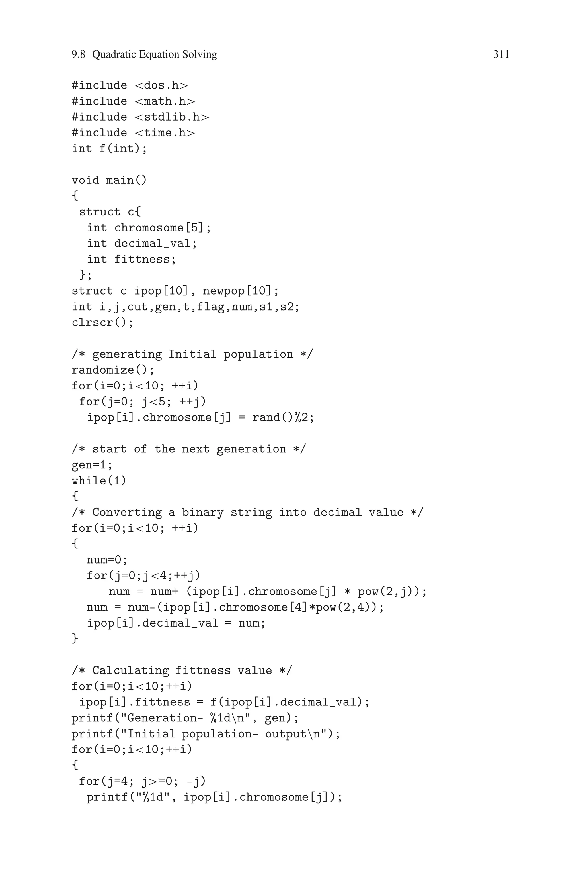
![9.8 Quadratic Equation Solving 311
#include dos.h
#include math.h
#include stdlib.h
#include time.h
int f(int);
void main()
{
struct c{
int chromosome[5];
int decimal_val;
int fittness;
};
struct c ipop[10], newpop[10];
int i,j,cut,gen,t,flag,num,s1,s2;
clrscr();
/* generating Initial population */
randomize();
for(i=0;i10; ++i)
for(j=0; j5; ++j)
ipop[i].chromosome[j] = rand()%2;
/* start of the next generation */
gen=1;
while(1)
{
/* Converting a binary string into decimal value */
for(i=0;i10; ++i)
{
num=0;
for(j=0;j4;++j)
num = num+ (ipop[i].chromosome[j] * pow(2,j));
num = num-(ipop[i].chromosome[4]*pow(2,4));
ipop[i].decimal_val = num;
}
/* Calculating fittness value */
for(i=0;i10;++i)
ipop[i].fittness = f(ipop[i].decimal_val);
printf(Generation- %1dn, gen);
printf(Initial population- outputn);
for(i=0;i10;++i)
{
for(j=4; j=0; –j)
printf(%1d, ipop[i].chromosome[j]);](https://image.slidesharecdn.com/s-220425101513/75/S-N-Sivanandam-S-N-Deepa-Introduction-to-Genetic-Algorithms-2008-ISBN-3540731894-pdf-323-2048.jpg)
![312 9 Genetic Algorithm Optimization in C/C++
printf( %d, ipop[i].decimal_val);
printf( %d, ipop[i].fittness);
printf(n);
}
for(i=0;i10; ++i)
{
if(ipop[i].fittness ==0)
{
printf(stop generationsn);
printf(result = %dn, ipop[i].decimal_val);
goto l1;
}
}
/* tournament selection */
printf(tournament selectionn );
i=0;
while(i=9)
{
s1 = rand()%10;
s2 = rand()%10;
printf(%d %d %d %dn, s1,s2,ipop[s1].fittness, ipop[s2].
fittness);
getche();
if( ipop[s1].fittness ipop[s2].fittness)
{
for(j=0;j5;++j)
newpop[i].chromosome[j] = ipop[s1].chromosome[j];
}
else
{
for(j=0;j5;++j)
newpop[i].chromosome[j] = ipop[s2].chromosome[j];
}
i++;
}
getche();
printf(new population -outputn);
for(i=0;i10;++i)
{
for(j=4; j=0; –j)
printf(%1d, newpop[i].chromosome[j]);
printf(n);
}
getche();](https://image.slidesharecdn.com/s-220425101513/75/S-N-Sivanandam-S-N-Deepa-Introduction-to-Genetic-Algorithms-2008-ISBN-3540731894-pdf-324-2048.jpg)
![9.8 Quadratic Equation Solving 313
/*crossover operation */
printf(crossover operationn);
printf(left/right cut-point positionn);
for(i=0;i=4;++i)
{
flag= rand()%2;
cut= rand()%5;
printf(%1d %1dn, flag, cut);
if(flag==0) /* crossover to left of cutpoint position*/
for(j=0;j=cut-1;++j)
{
t=newpop[2*i].chromosome[j];
newpop[2*i].chromosome[j]= newpop[(2*i+1)].
chromosome[j];
newpop[(2*i+1)].chromosome[j]= t;
}
else /* crossover to the right of cutpoint position*/
for(j=cut+1;j=4;++j)
{
t=newpop[2*i].chromosome[j];
newpop[2*i].chromosome[j]= newpop[(2*i+1)].
chromosome[j];
newpop[(2*i+1)].chromosome[j]= t;
}
for(j=4; j=0; –j)
printf(%1d, newpop[2*i].chromosome[j]);
printf(n);
for(j=4; j=0; –j)
printf(%1d, newpop[2*i+1].chromosome[j]);
printf(n);
}
/* copy newpopulation to initial population*/
for(i=0; i10; ++i)
{
for(j=0; j5;++j)
ipop[i].chromosome[j] = newpop[i].chromosome[j];
}
gen=gen+1;
}
l1:
printf(endn);
}
int f(int x)
{
return ( x*x + 5*x + 6);
}](https://image.slidesharecdn.com/s-220425101513/75/S-N-Sivanandam-S-N-Deepa-Introduction-to-Genetic-Algorithms-2008-ISBN-3540731894-pdf-325-2048.jpg)
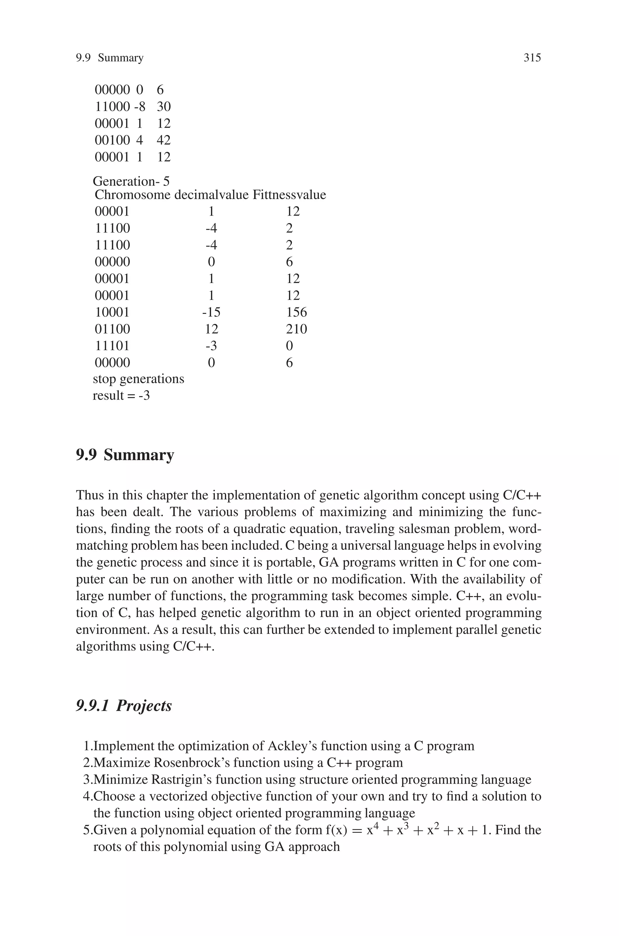
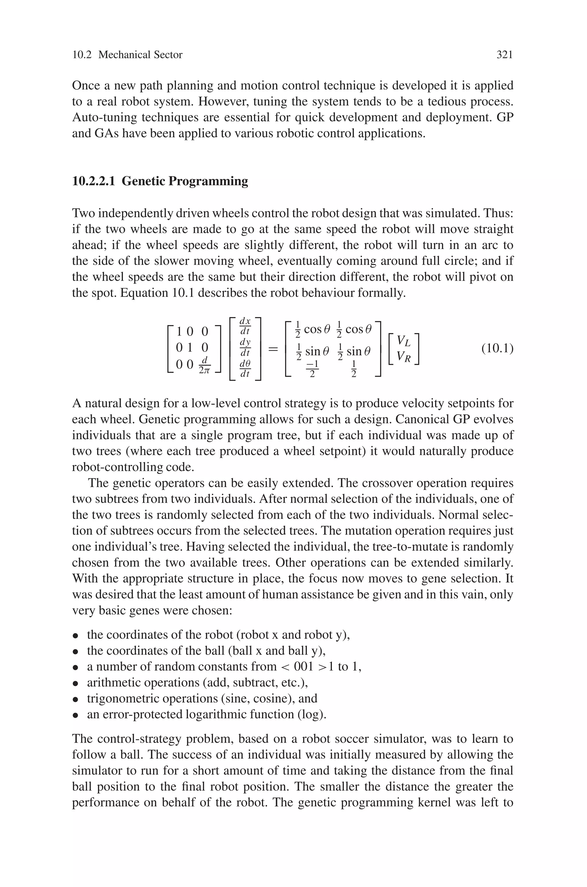
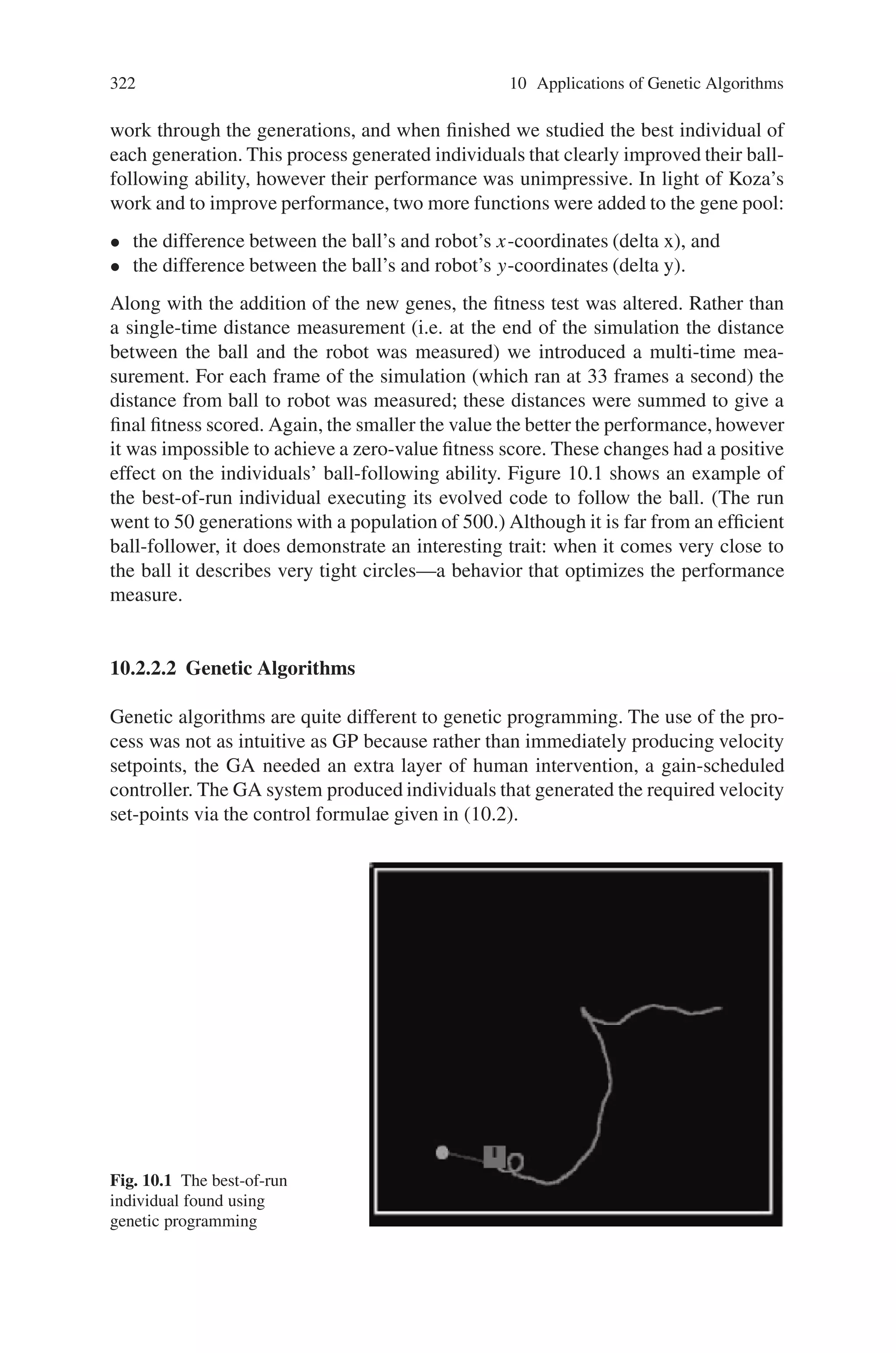
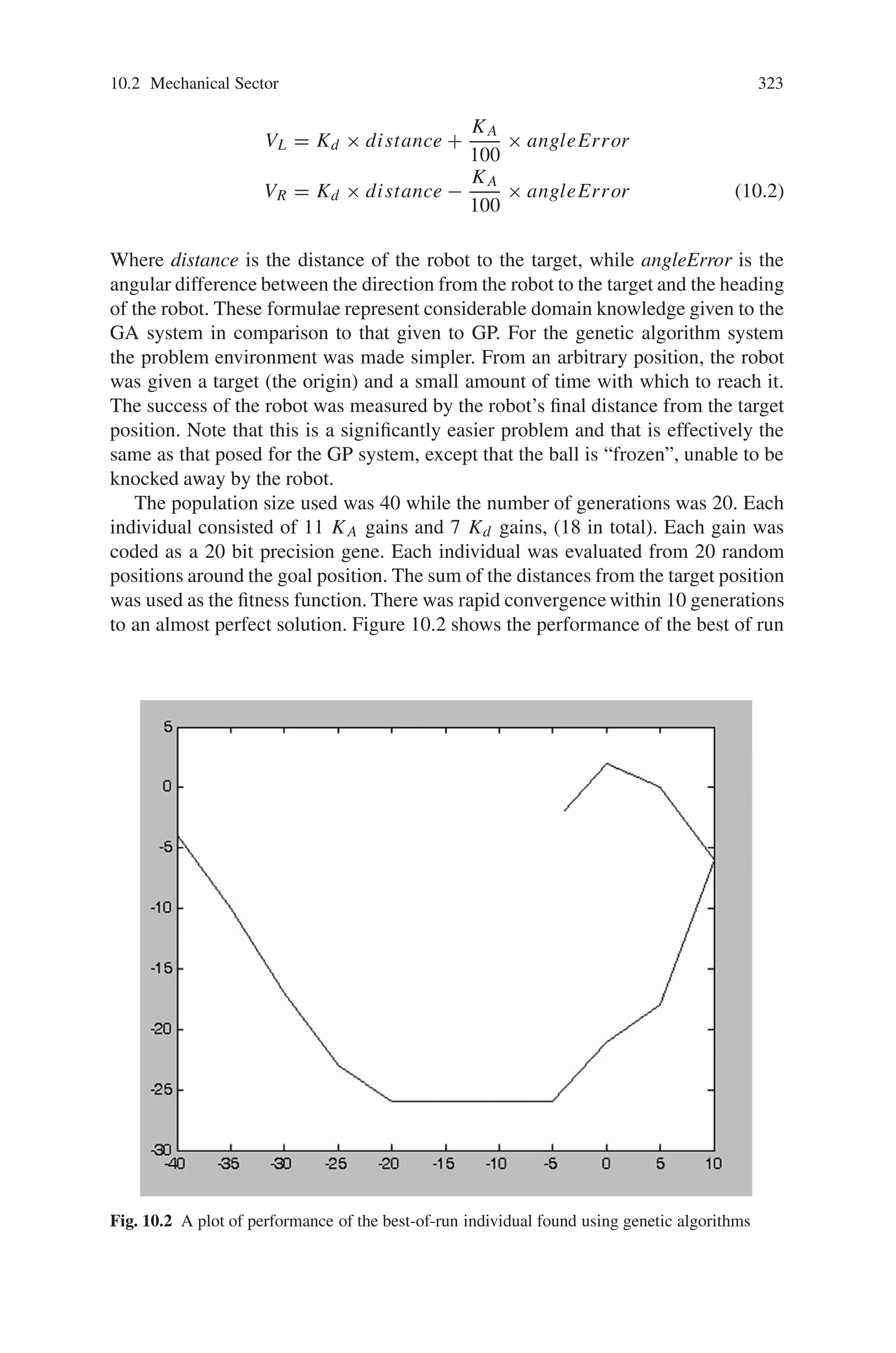
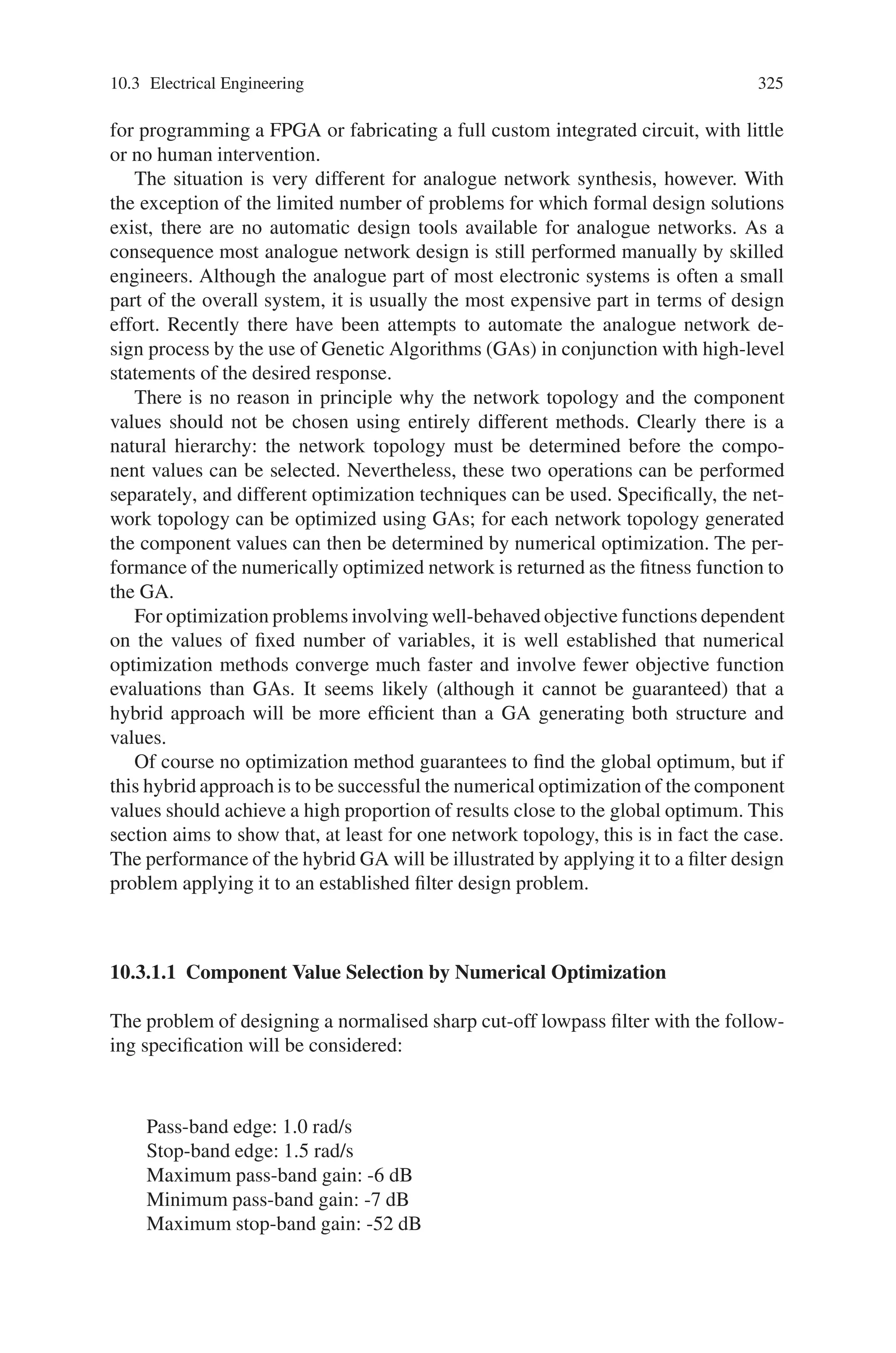
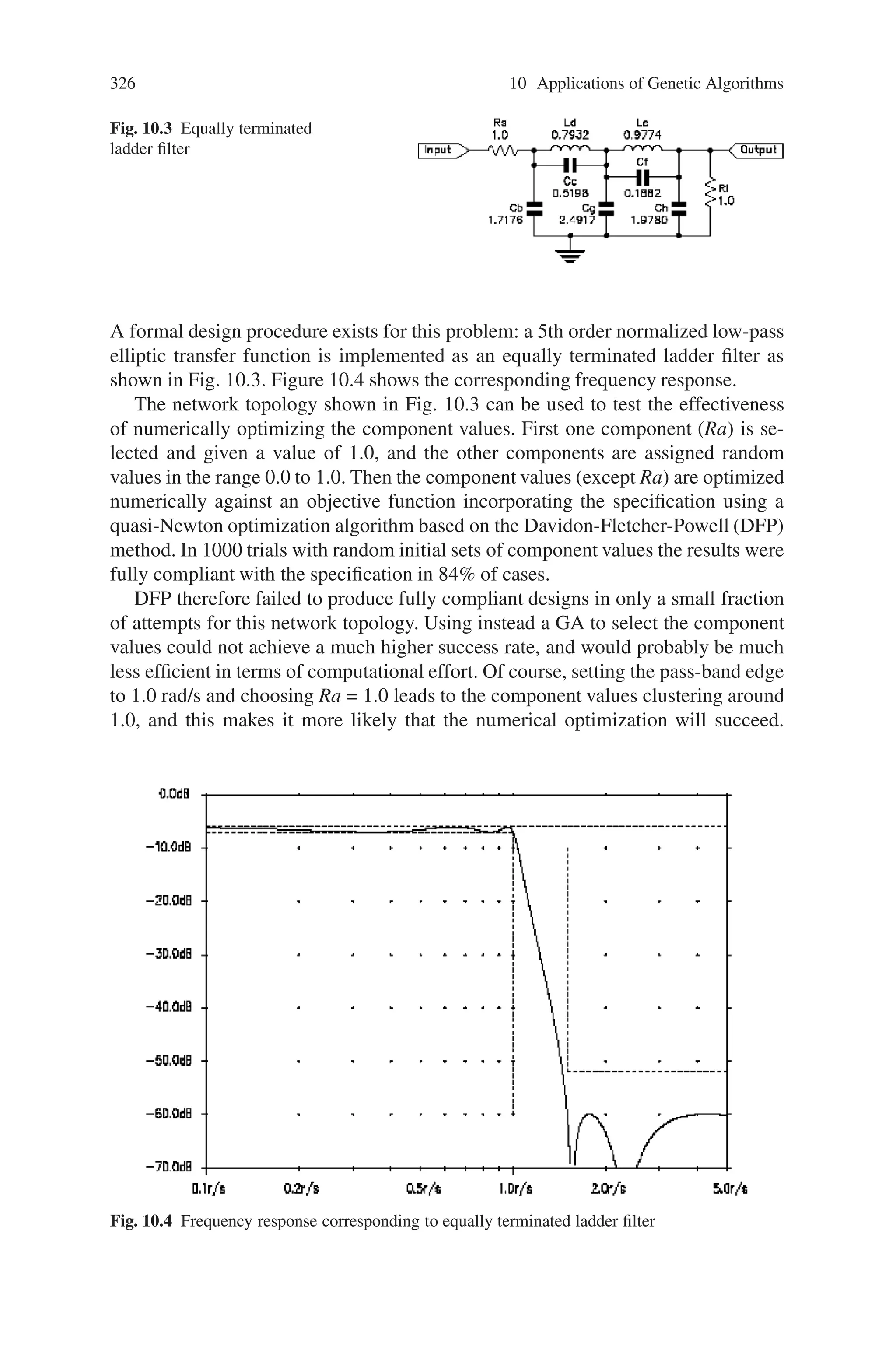
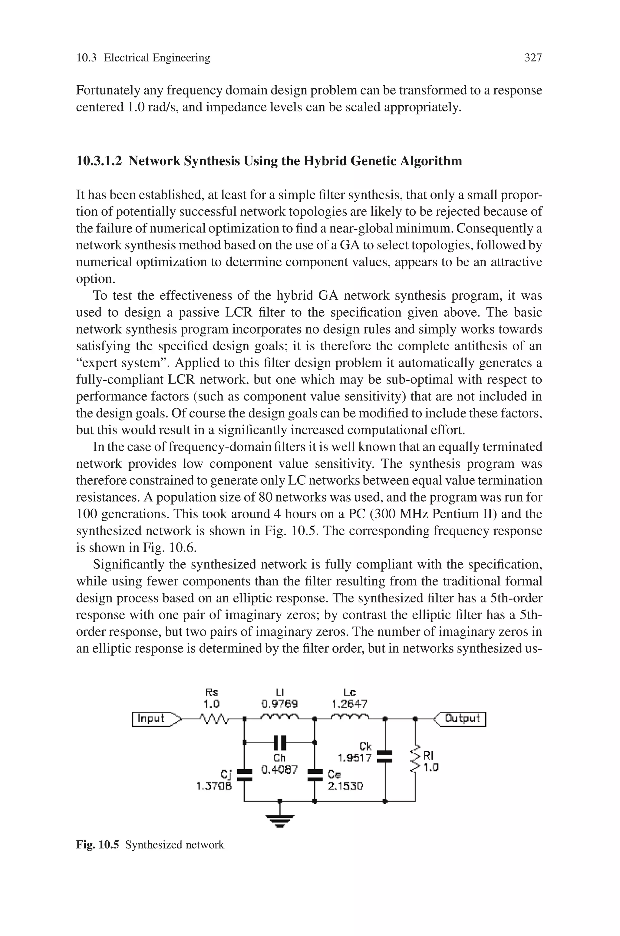
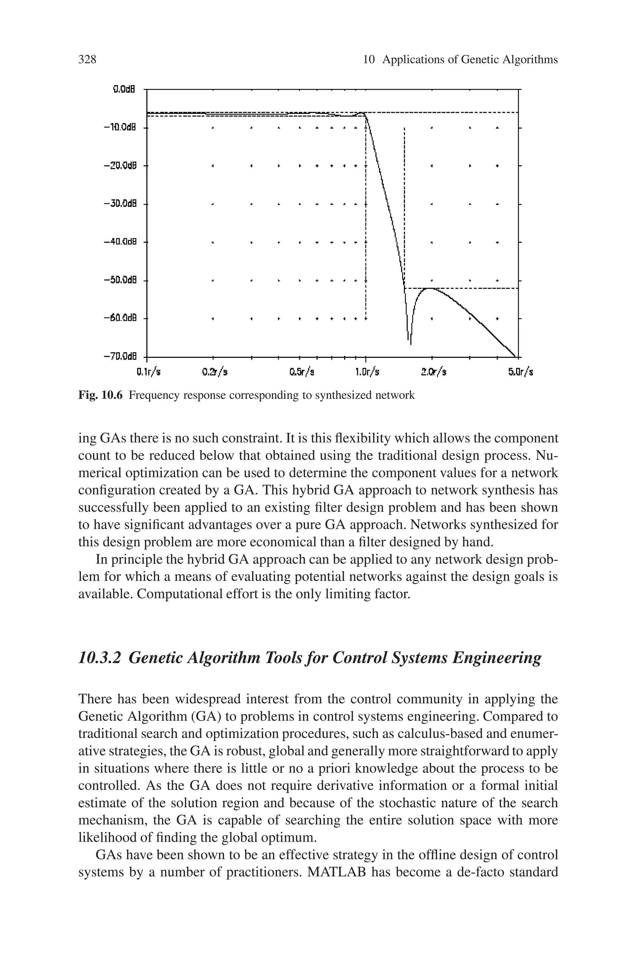
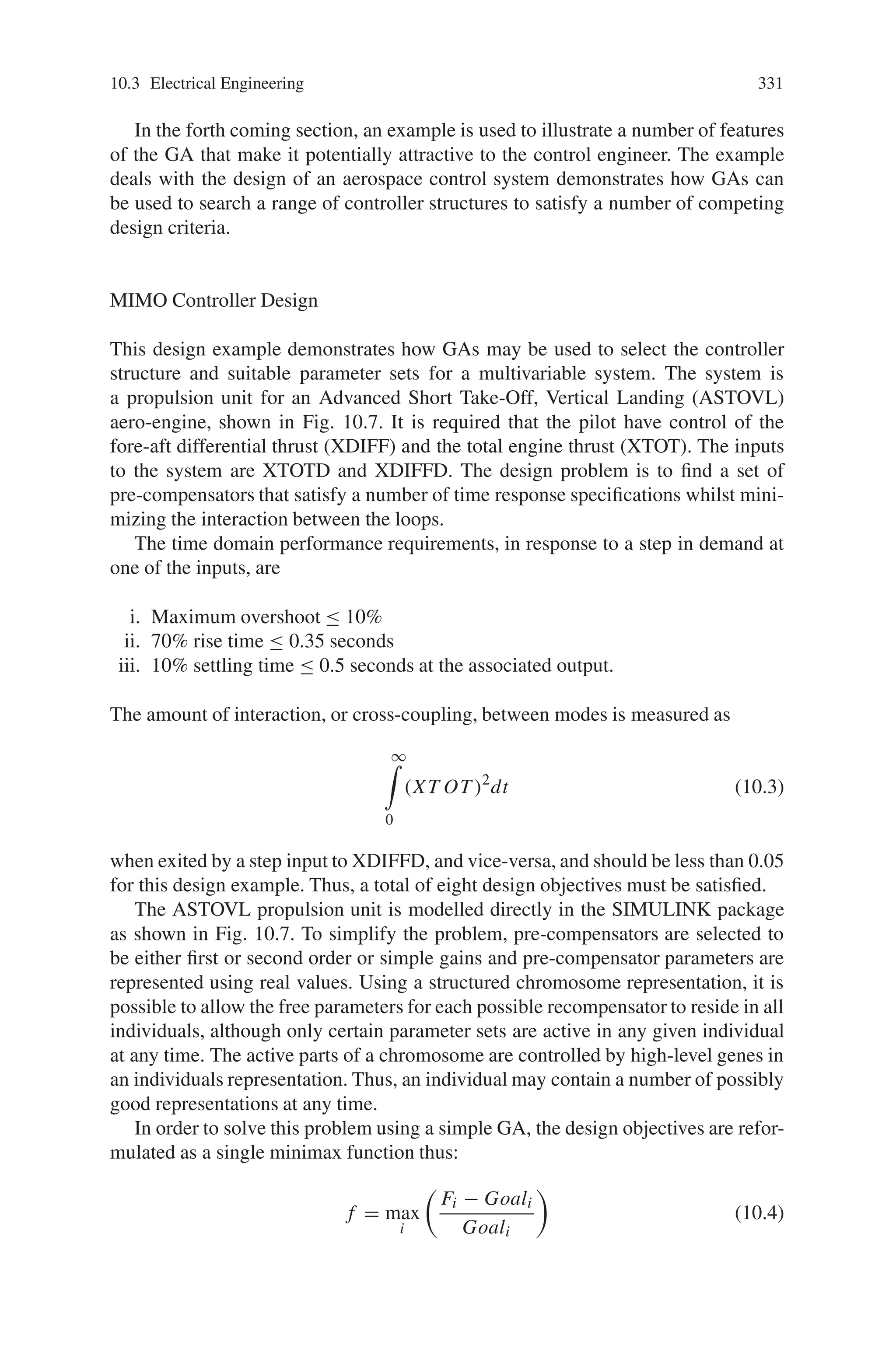
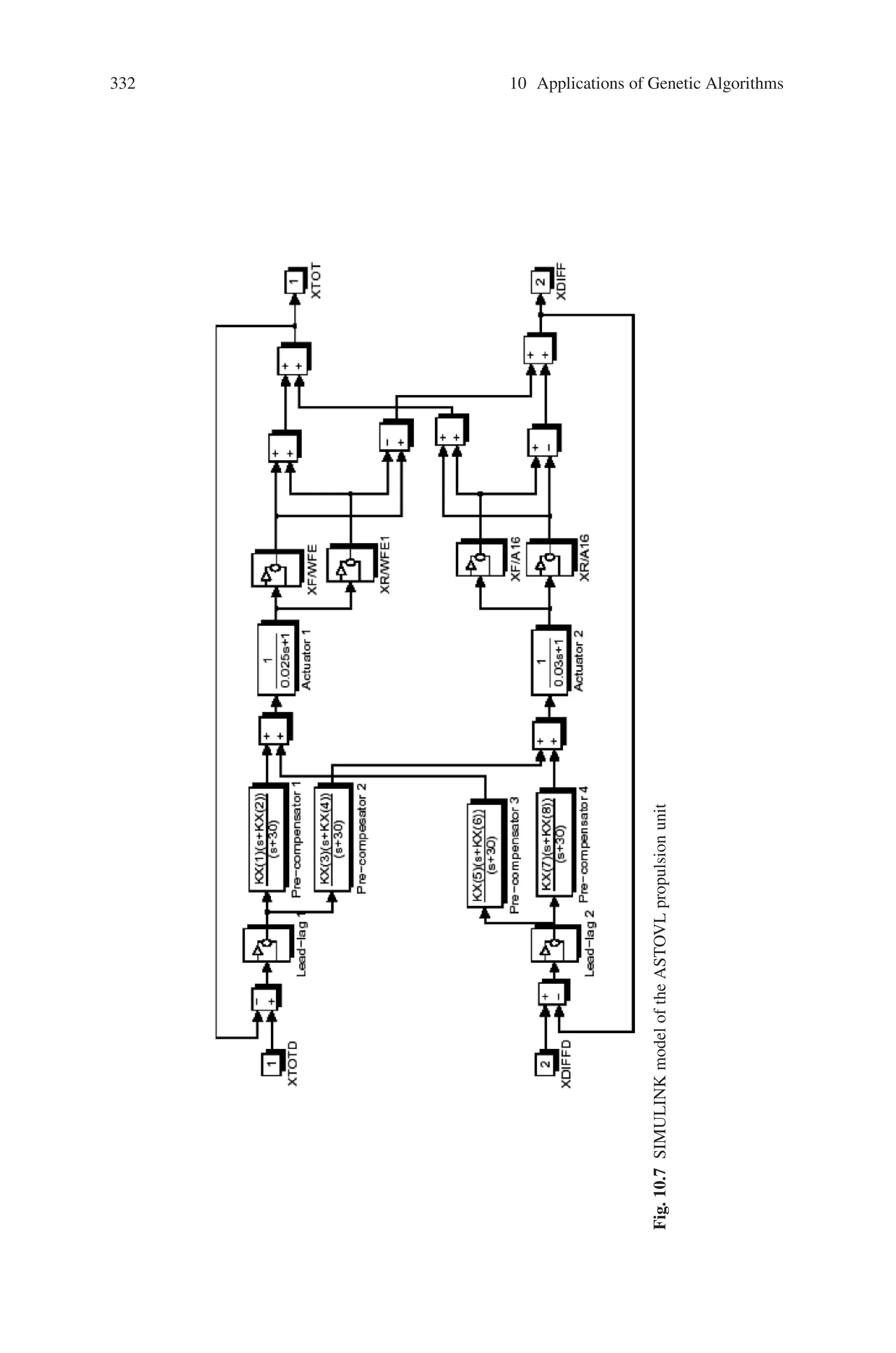
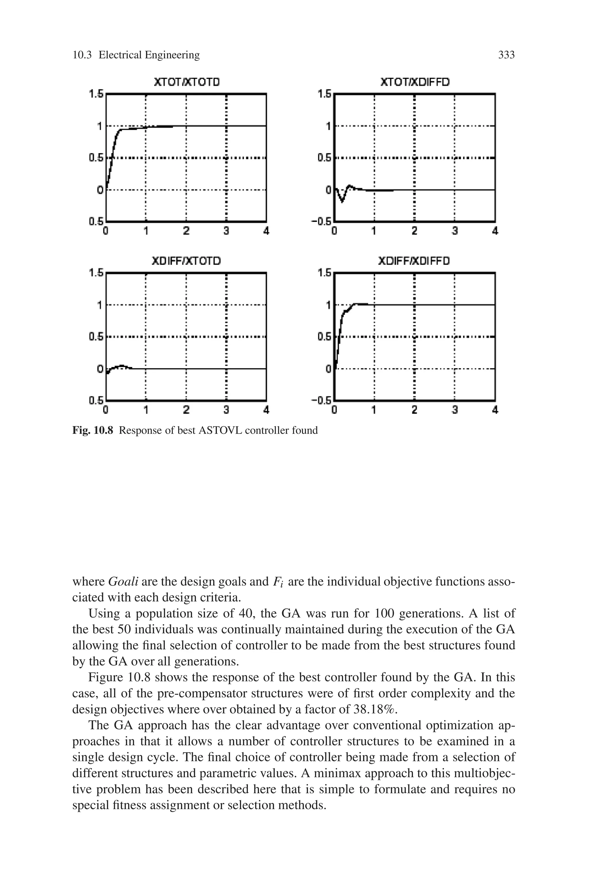
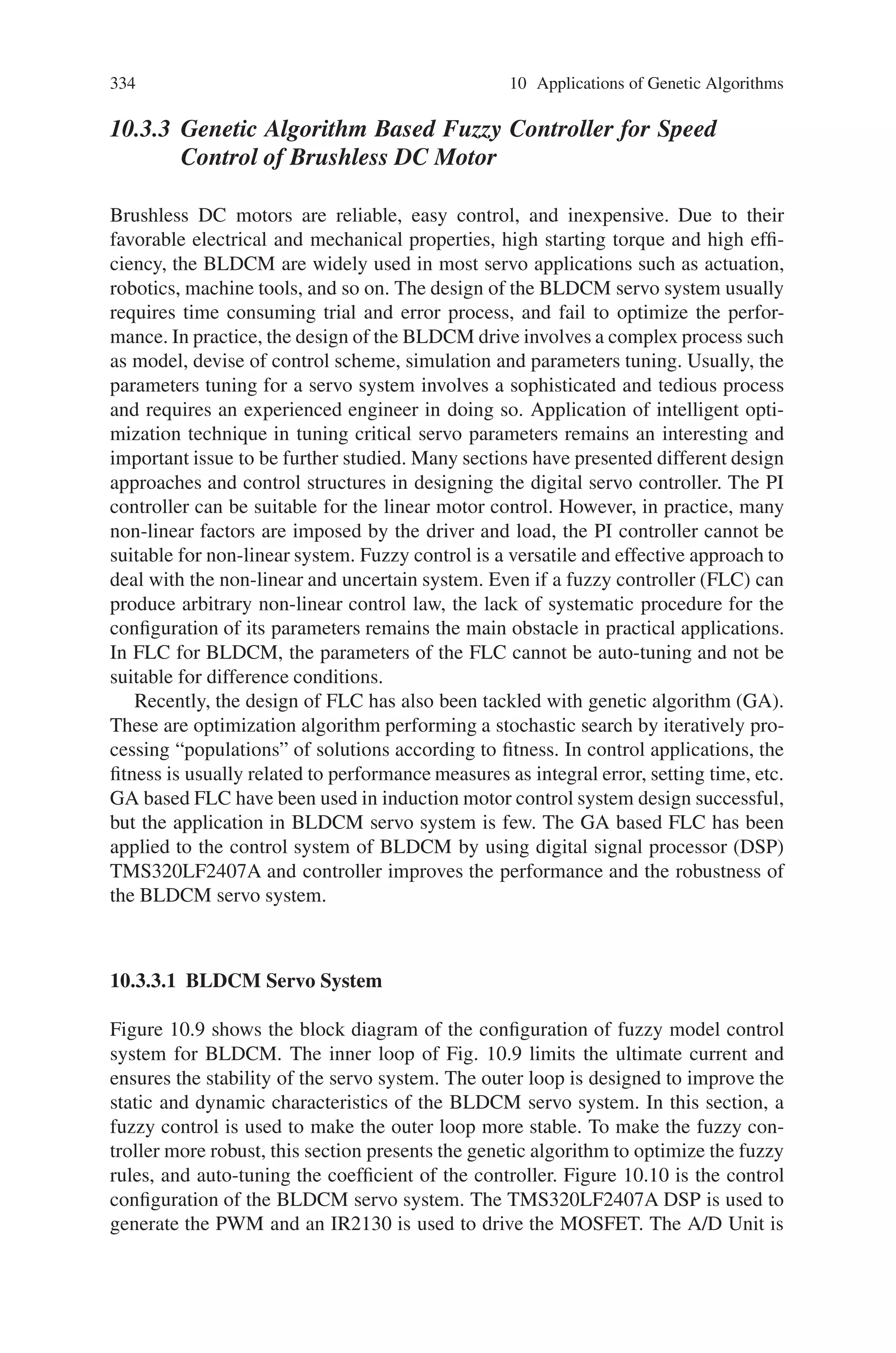
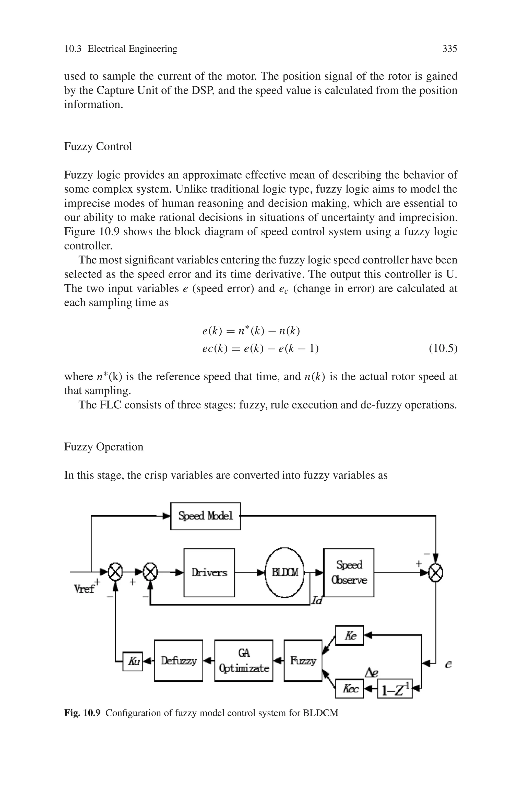
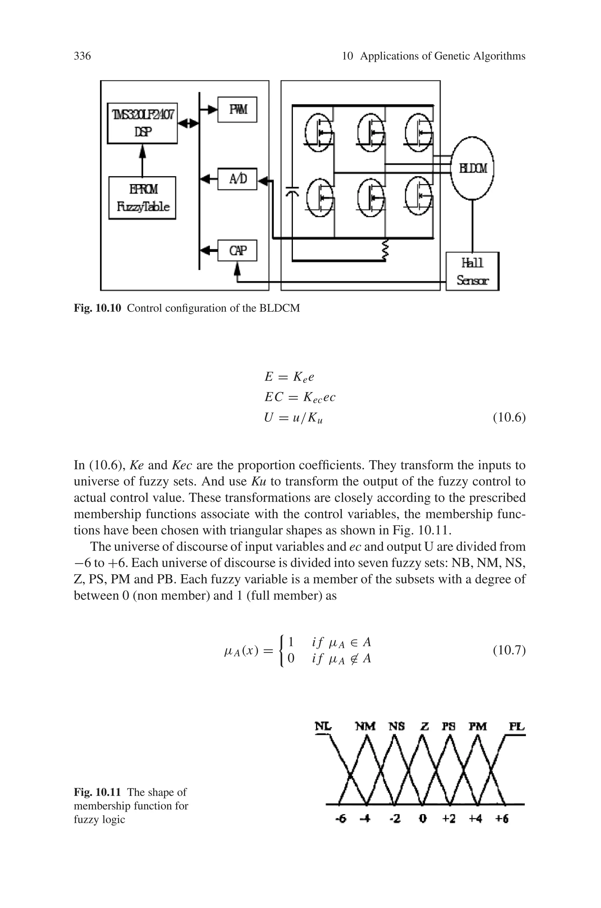
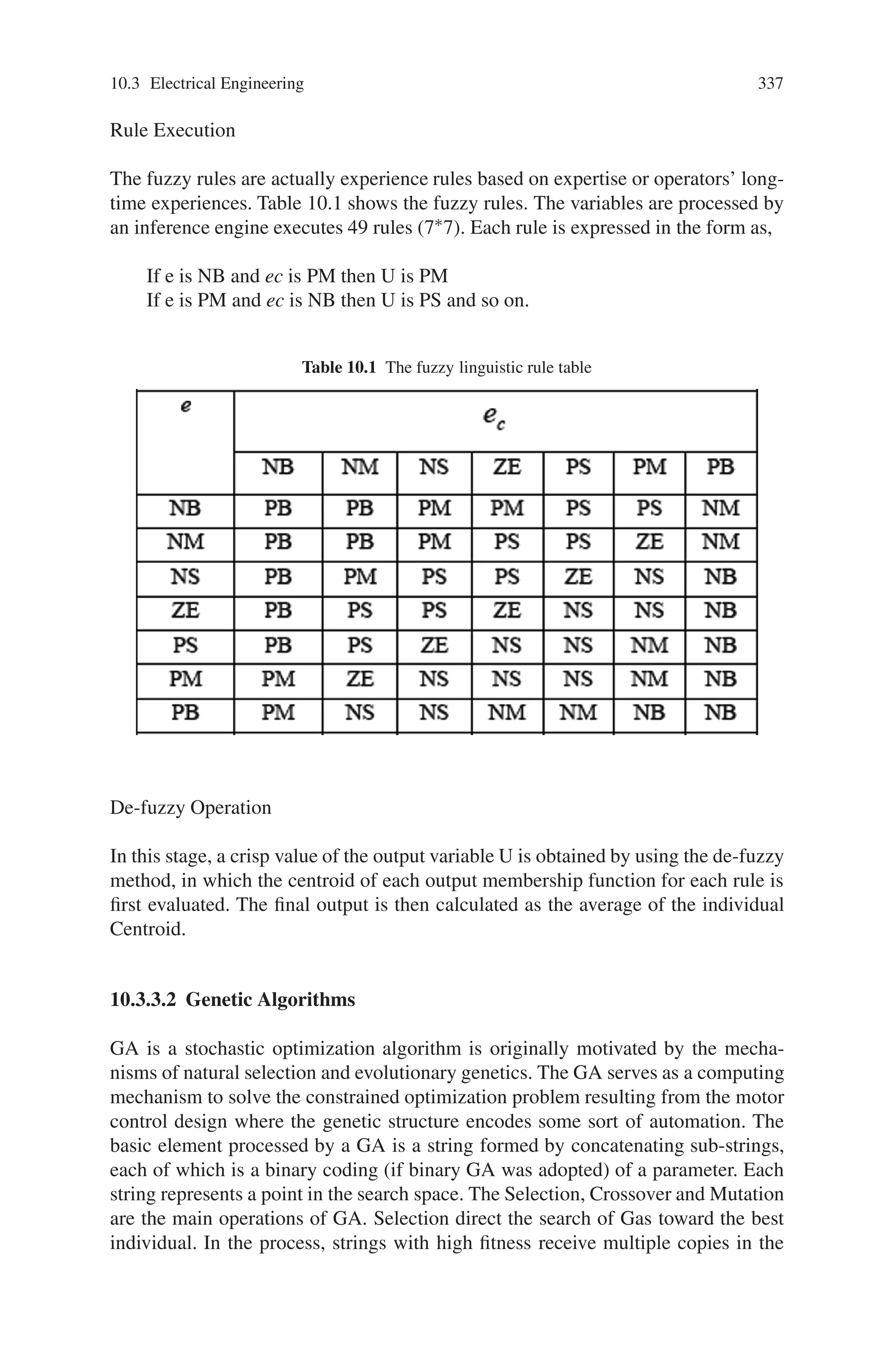
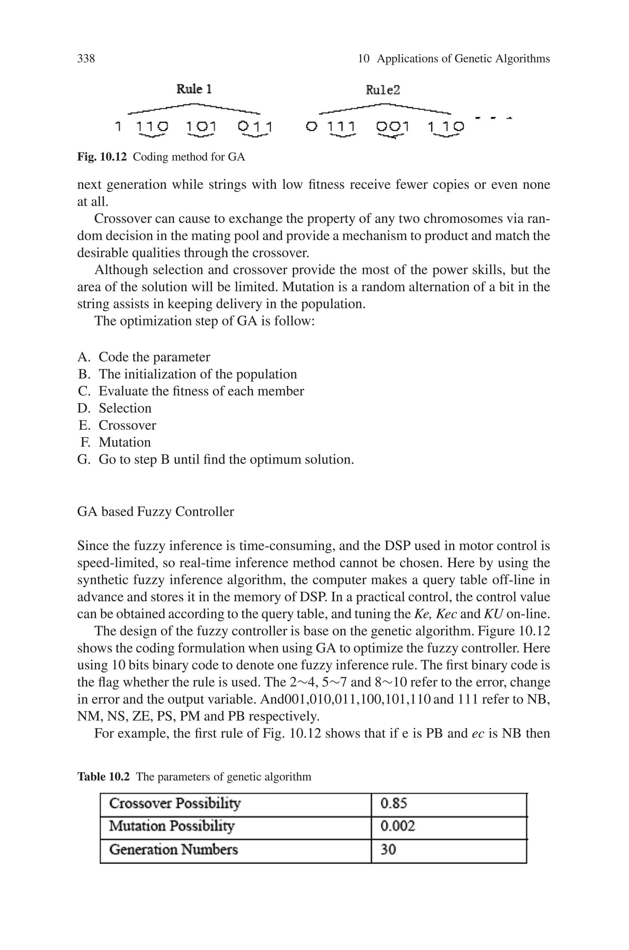
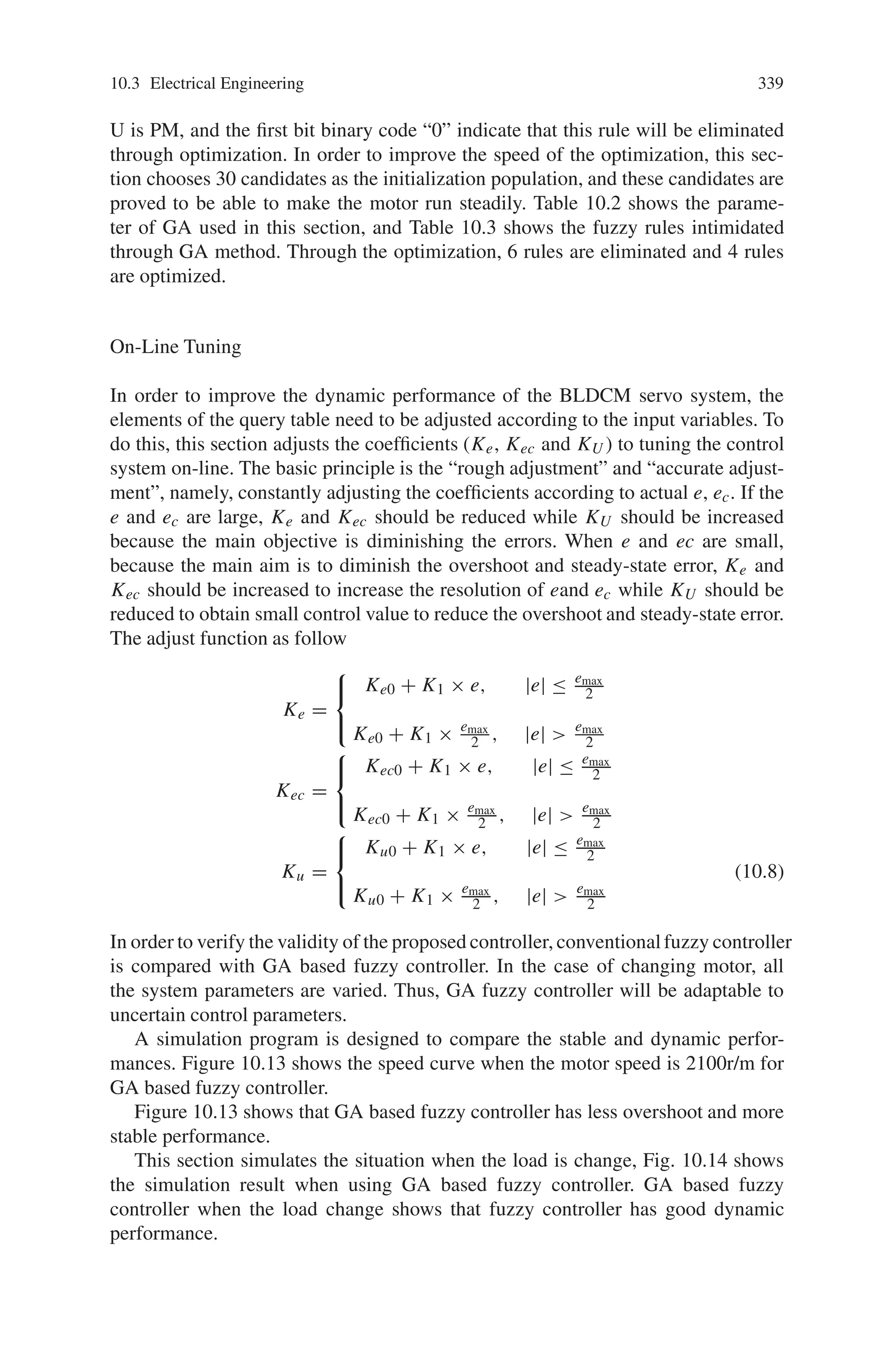
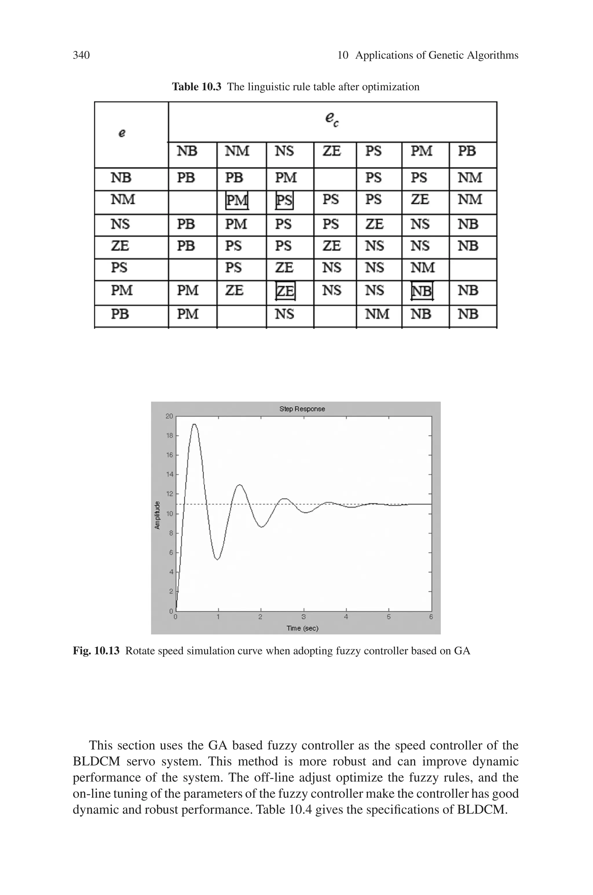
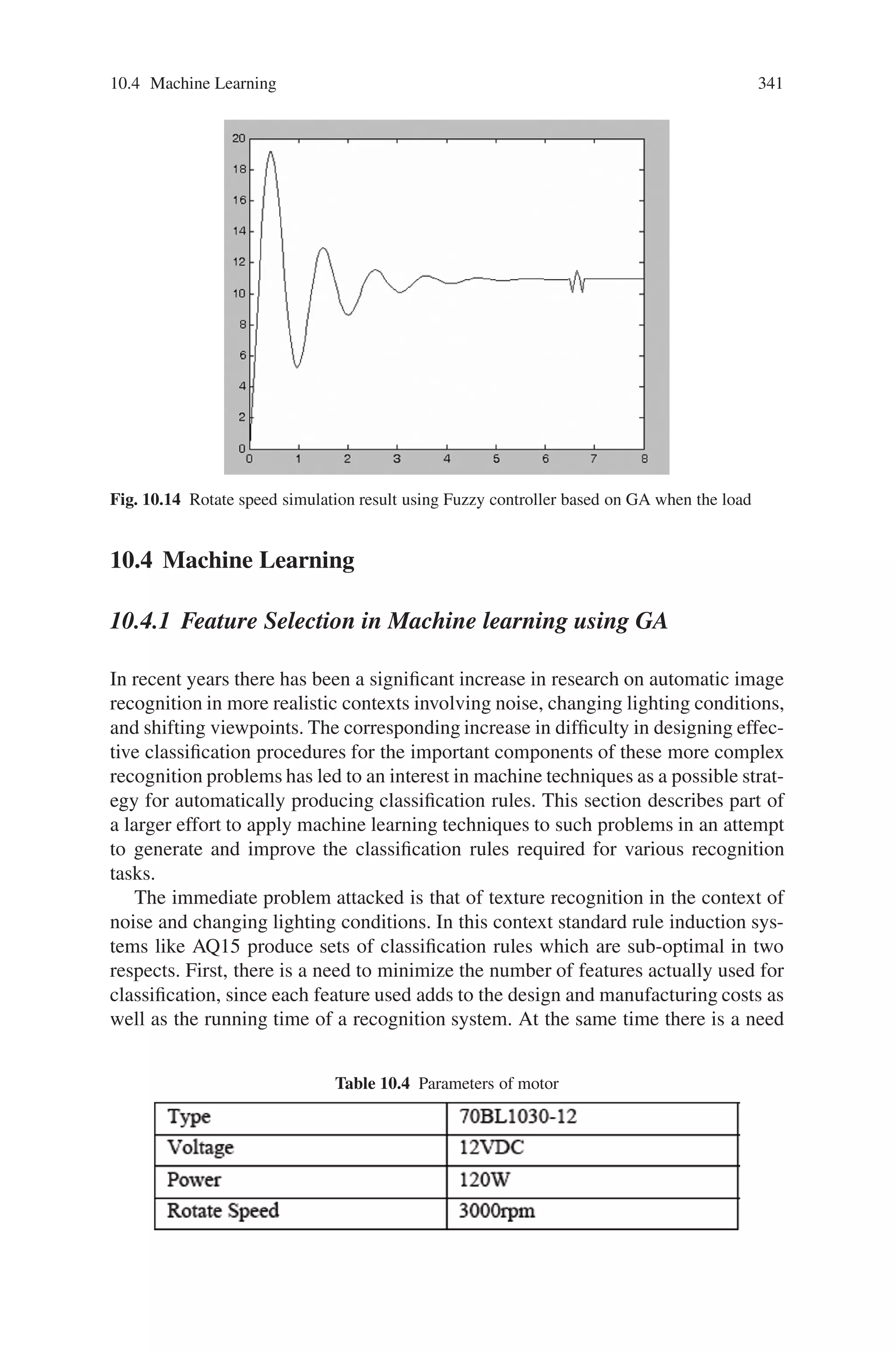
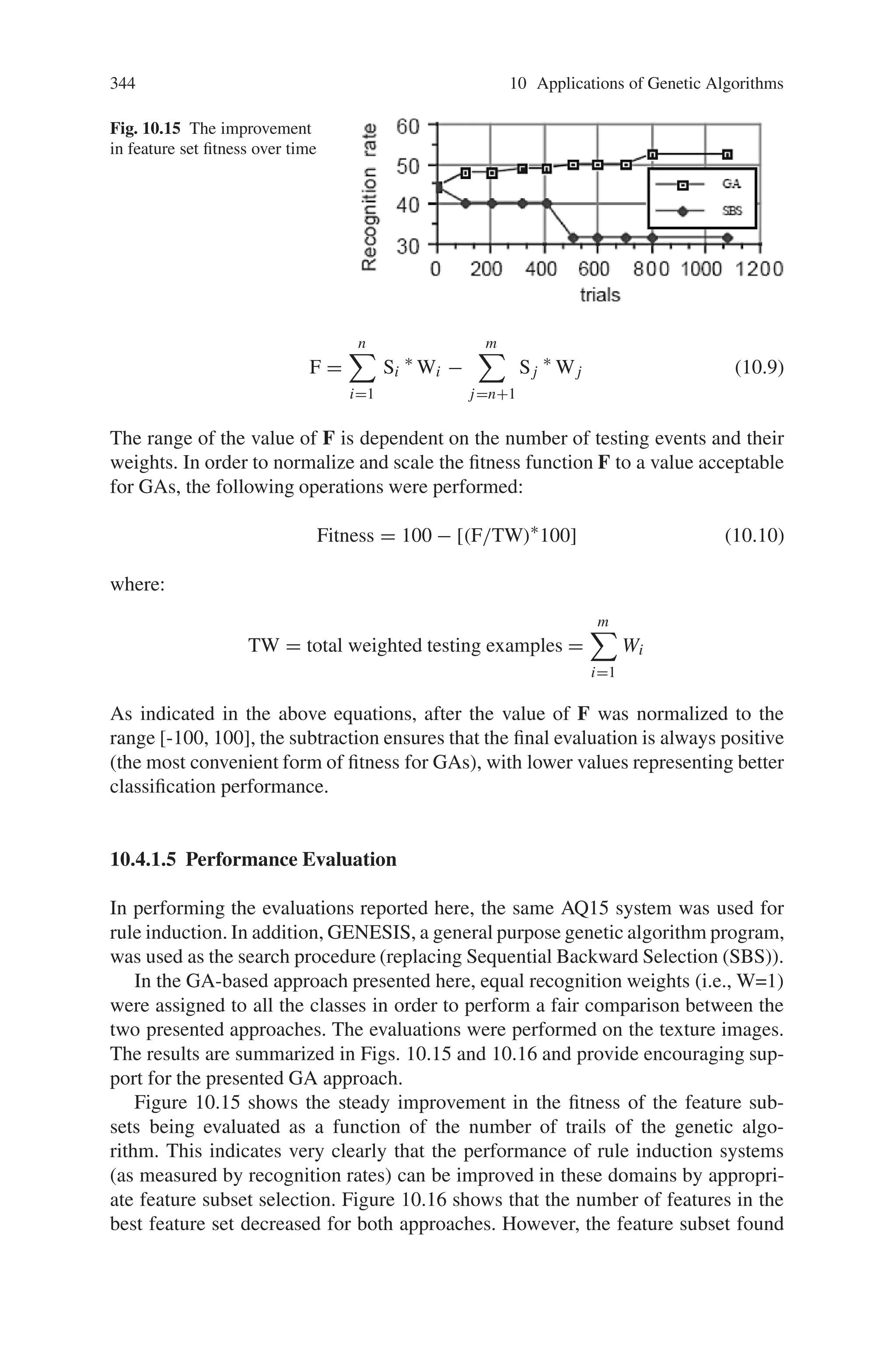
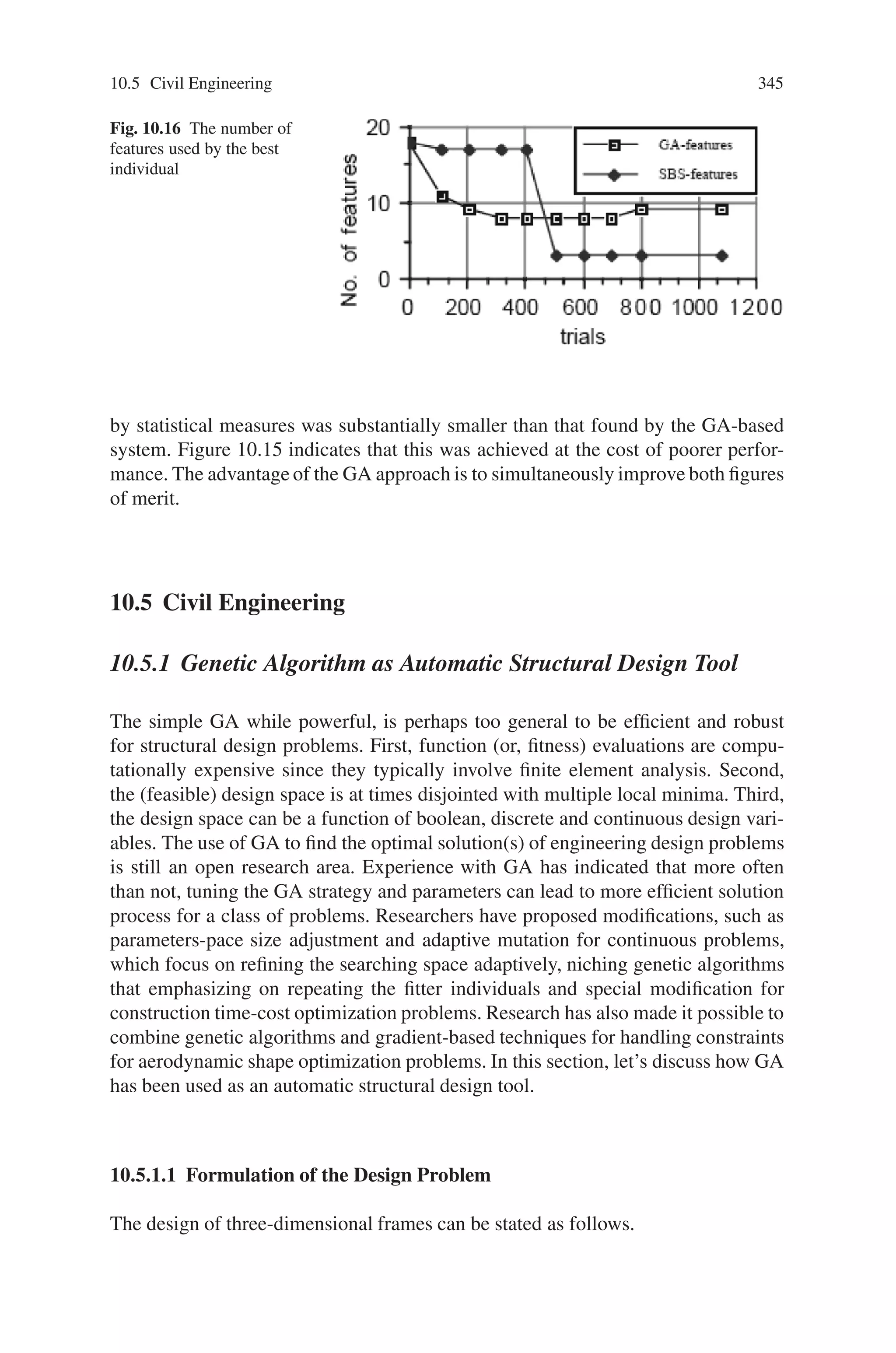
![344 10 Applications of Genetic Algorithms
Fig. 10.15 The improvement
in feature set fitness over time
F =
n
i=1
Si
∗
Wi −
m
j=n+1
Sj
∗
Wj (10.9)
The range of the value of F is dependent on the number of testing events and their
weights. In order to normalize and scale the fitness function F to a value acceptable
for GAs, the following operations were performed:
Fitness = 100 − [(F/TW)∗
100] (10.10)
where:
TW = total weighted testing examples =
m
i=1
Wi
As indicated in the above equations, after the value of F was normalized to the
range [-100, 100], the subtraction ensures that the final evaluation is always positive
(the most convenient form of fitness for GAs), with lower values representing better
classification performance.
10.4.1.5 Performance Evaluation
In performing the evaluations reported here, the same AQ15 system was used for
rule induction. In addition, GENESIS, a general purpose genetic algorithm program,
was used as the search procedure (replacing Sequential Backward Selection (SBS)).
In the GA-based approach presented here, equal recognition weights (i.e., W=1)
were assigned to all the classes in order to perform a fair comparison between the
two presented approaches. The evaluations were performed on the texture images.
The results are summarized in Figs. 10.15 and 10.16 and provide encouraging sup-
port for the presented GA approach.
Figure 10.15 shows the steady improvement in the fitness of the feature sub-
sets being evaluated as a function of the number of trails of the genetic algo-
rithm. This indicates very clearly that the performance of rule induction systems
(as measured by recognition rates) can be improved in these domains by appropri-
ate feature subset selection. Figure 10.16 shows that the number of features in the
best feature set decreased for both approaches. However, the feature subset found](https://image.slidesharecdn.com/s-220425101513/75/S-N-Sivanandam-S-N-Deepa-Introduction-to-Genetic-Algorithms-2008-ISBN-3540731894-pdf-357-2048.jpg)
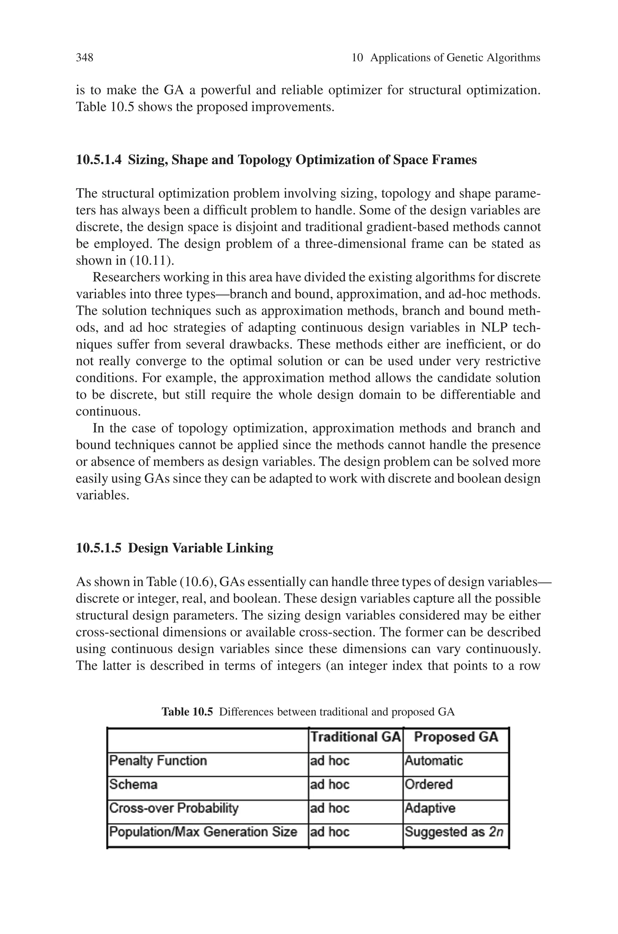

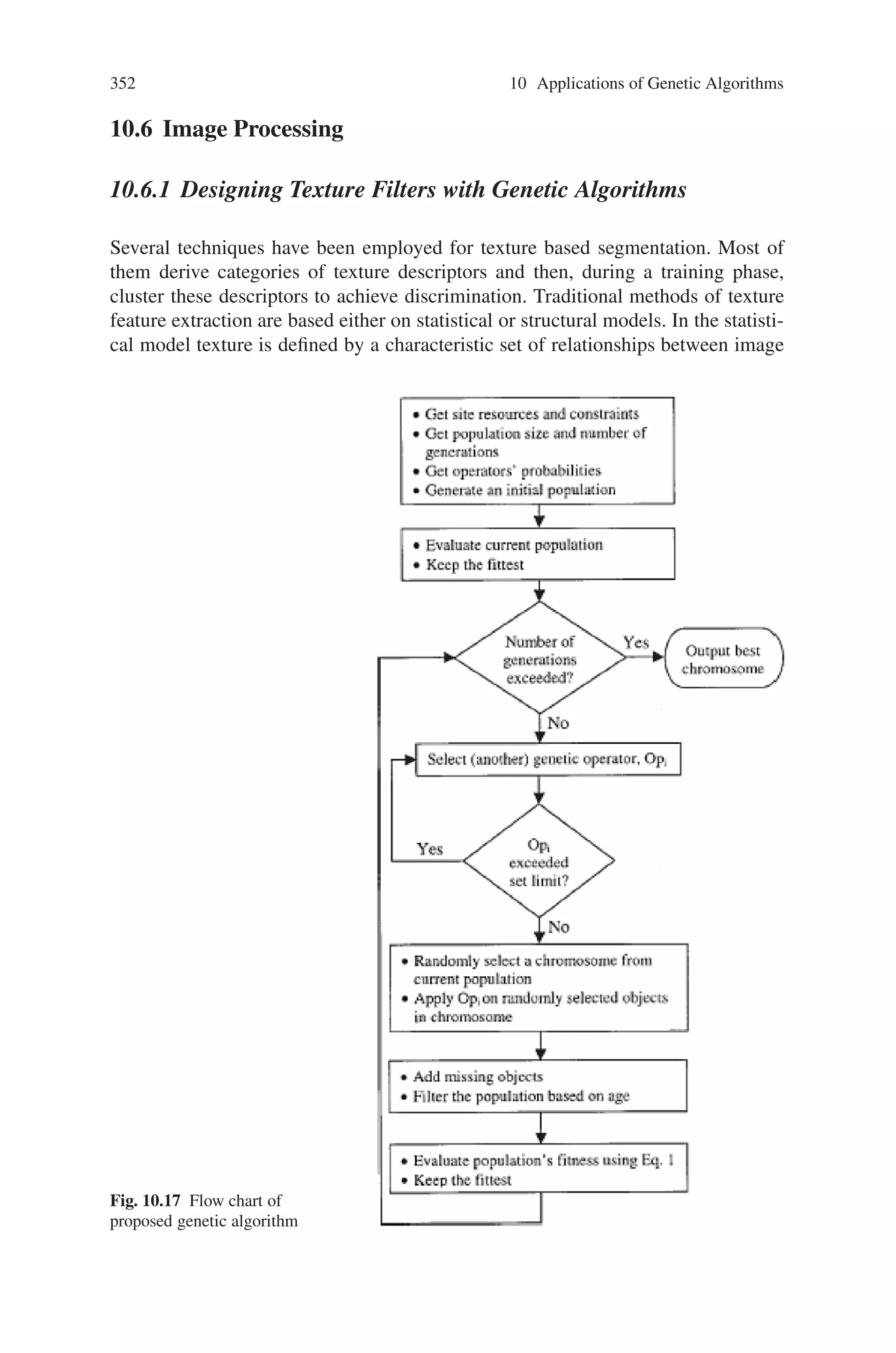
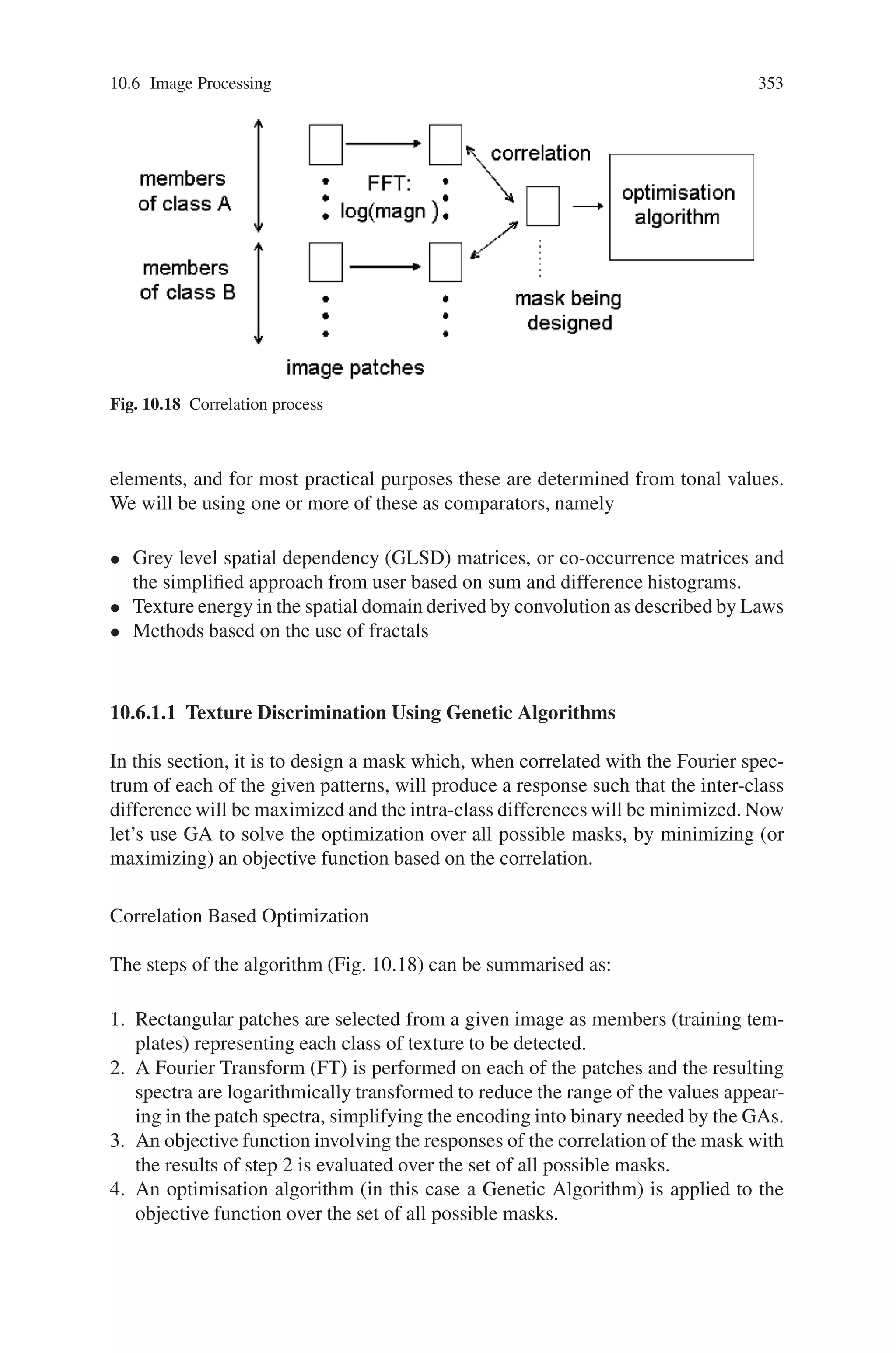

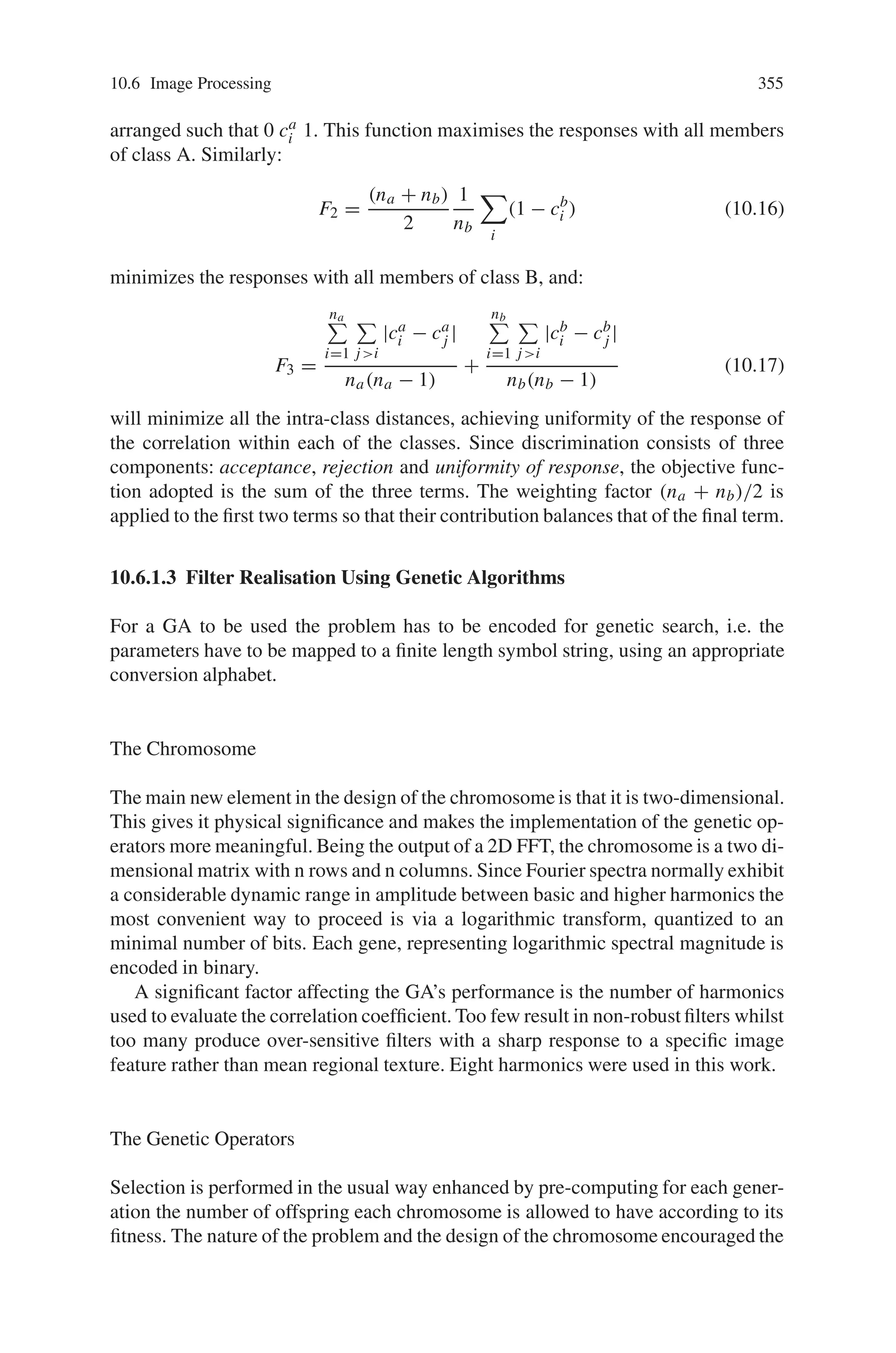
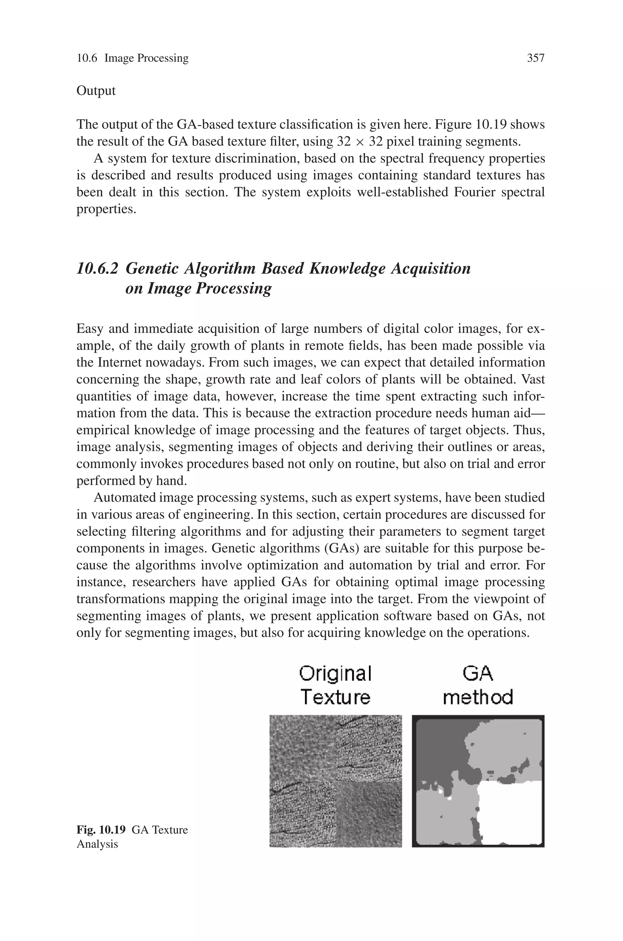
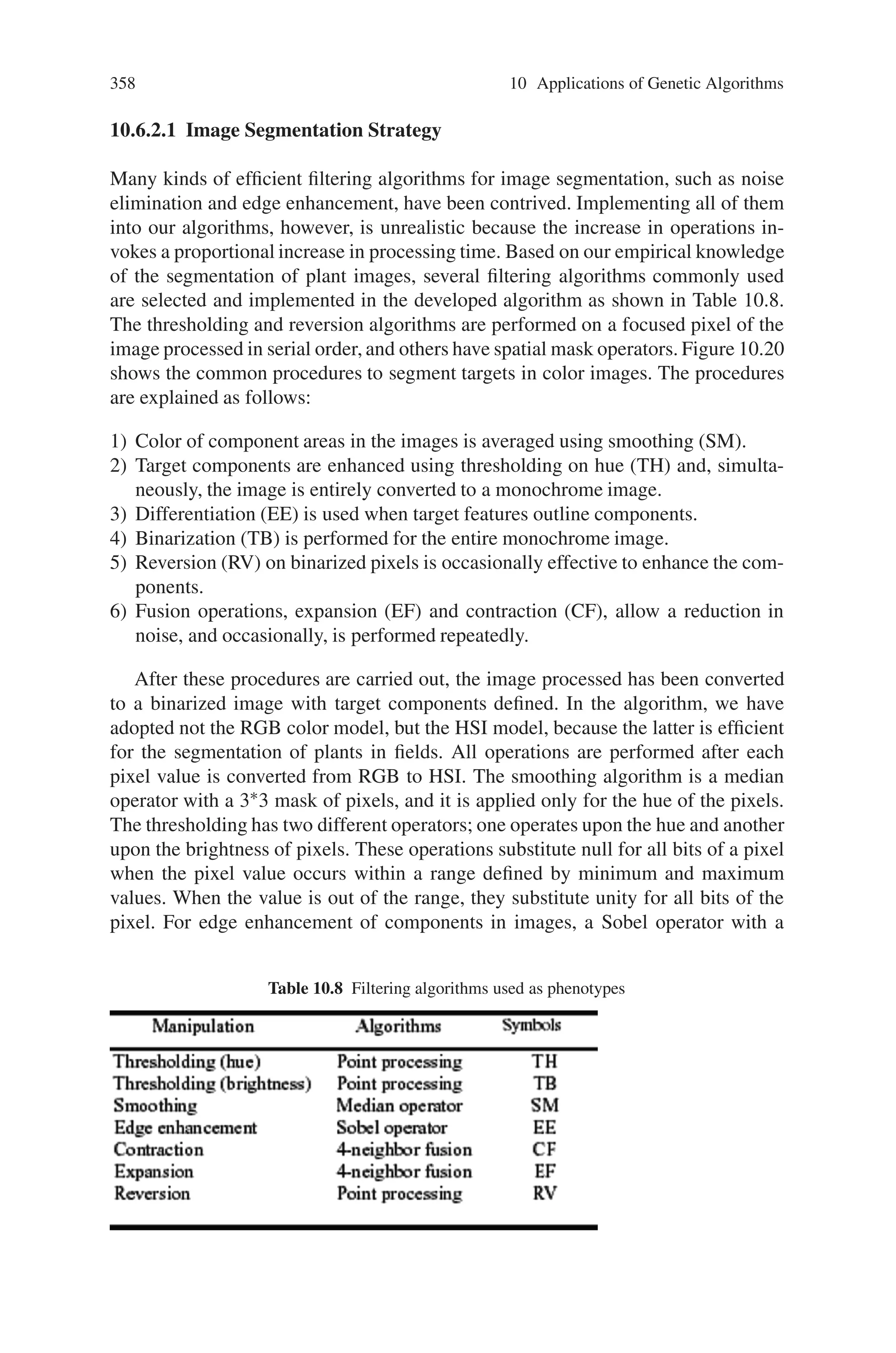
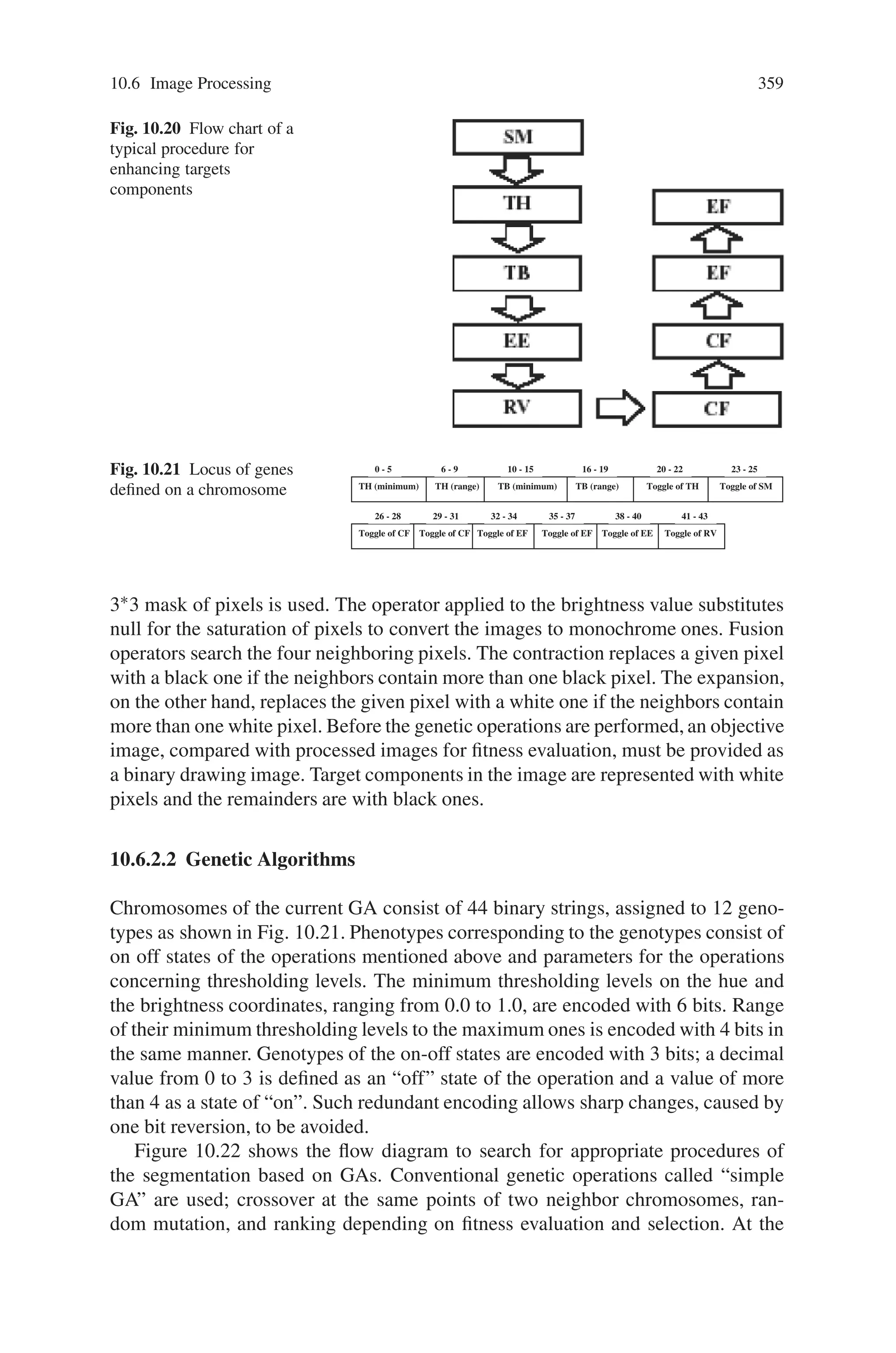
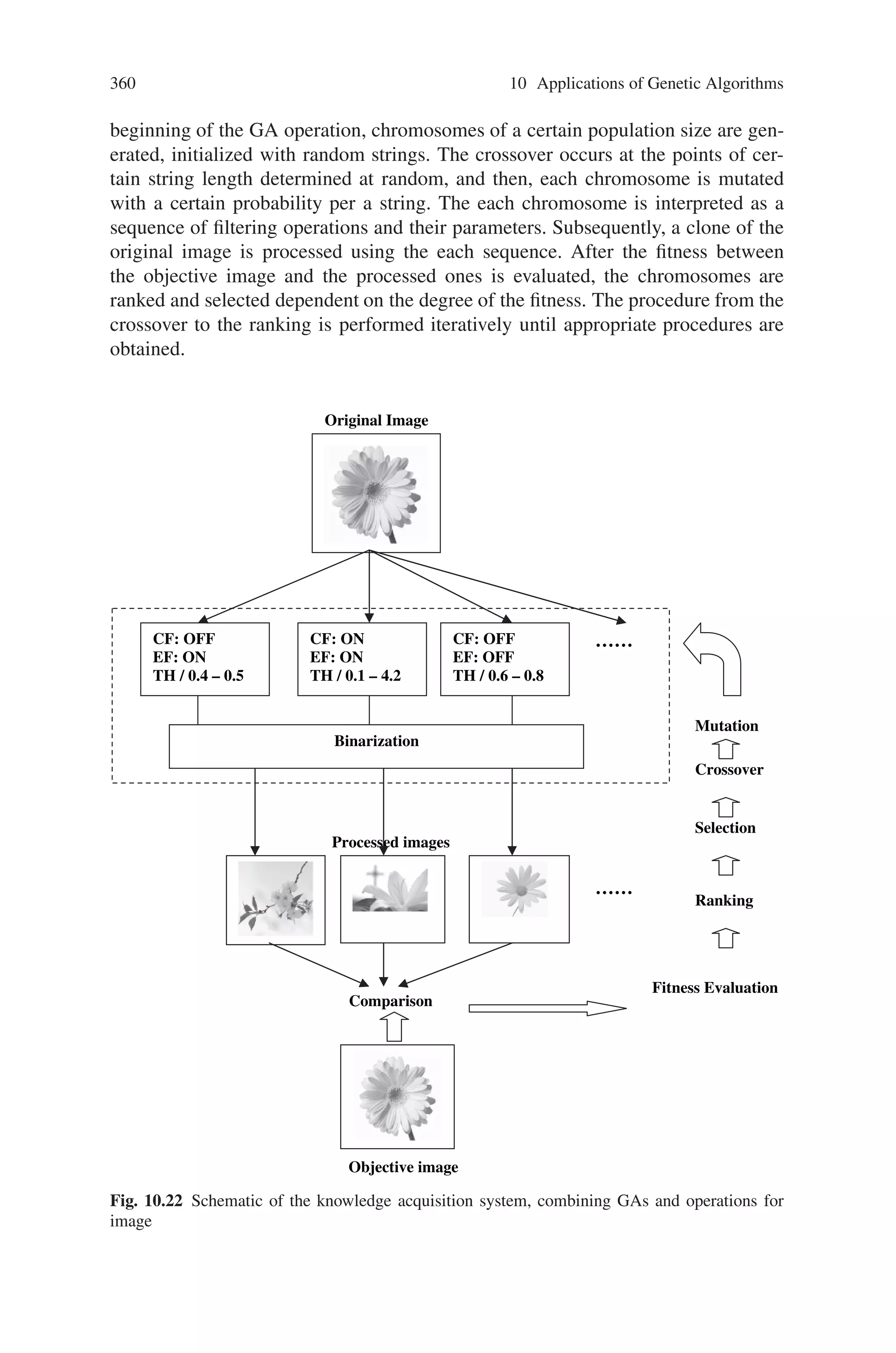
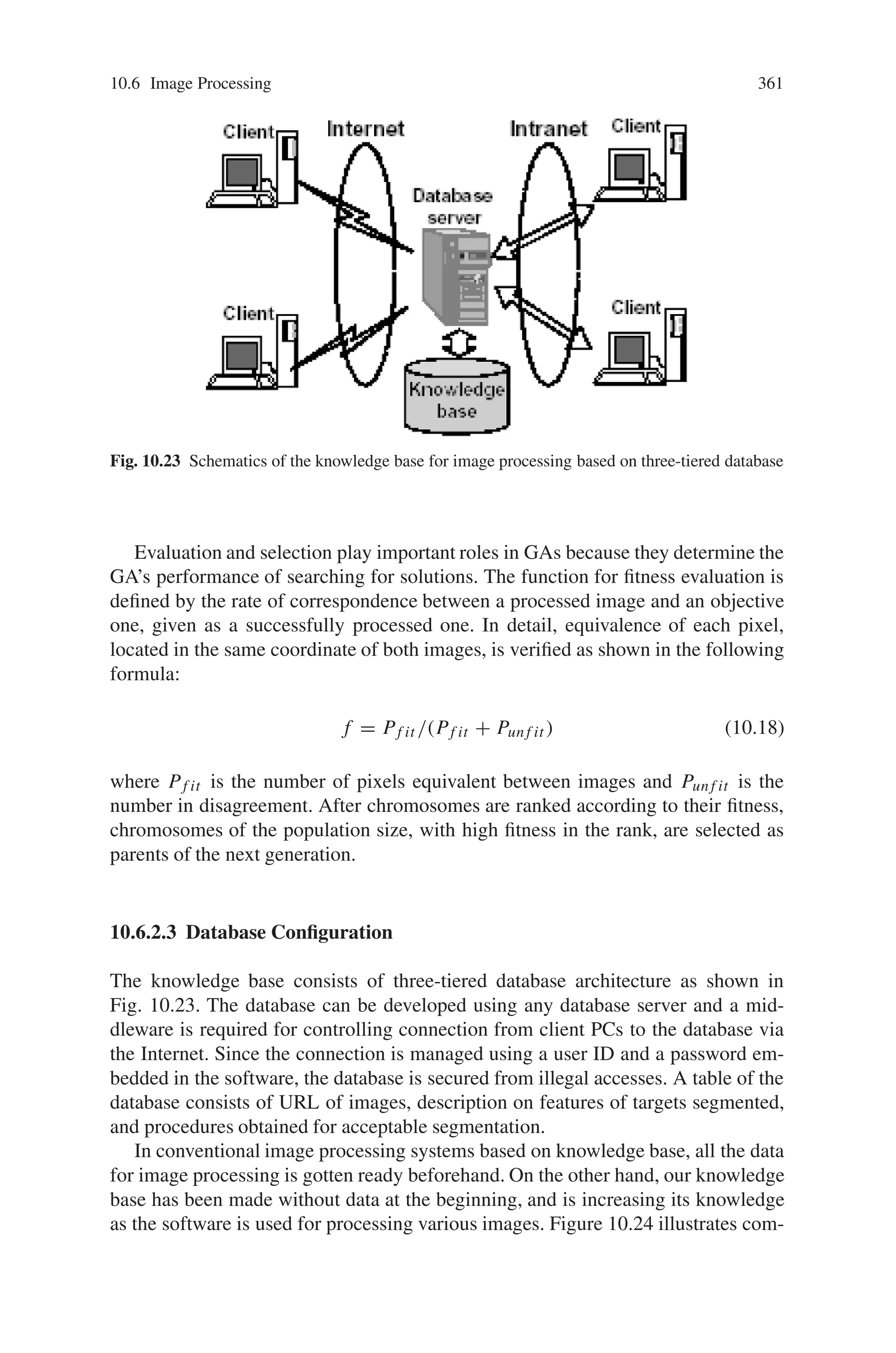
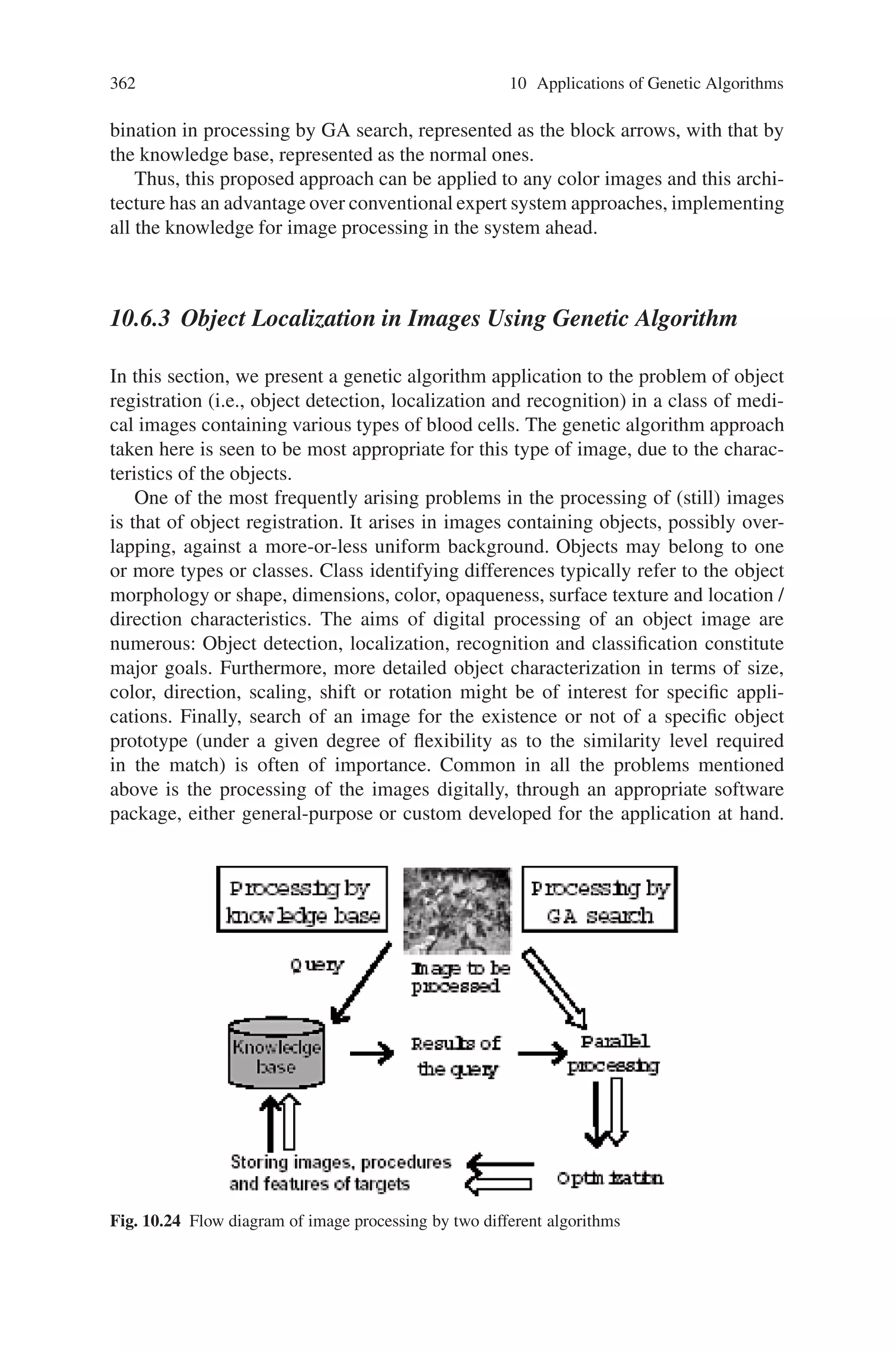
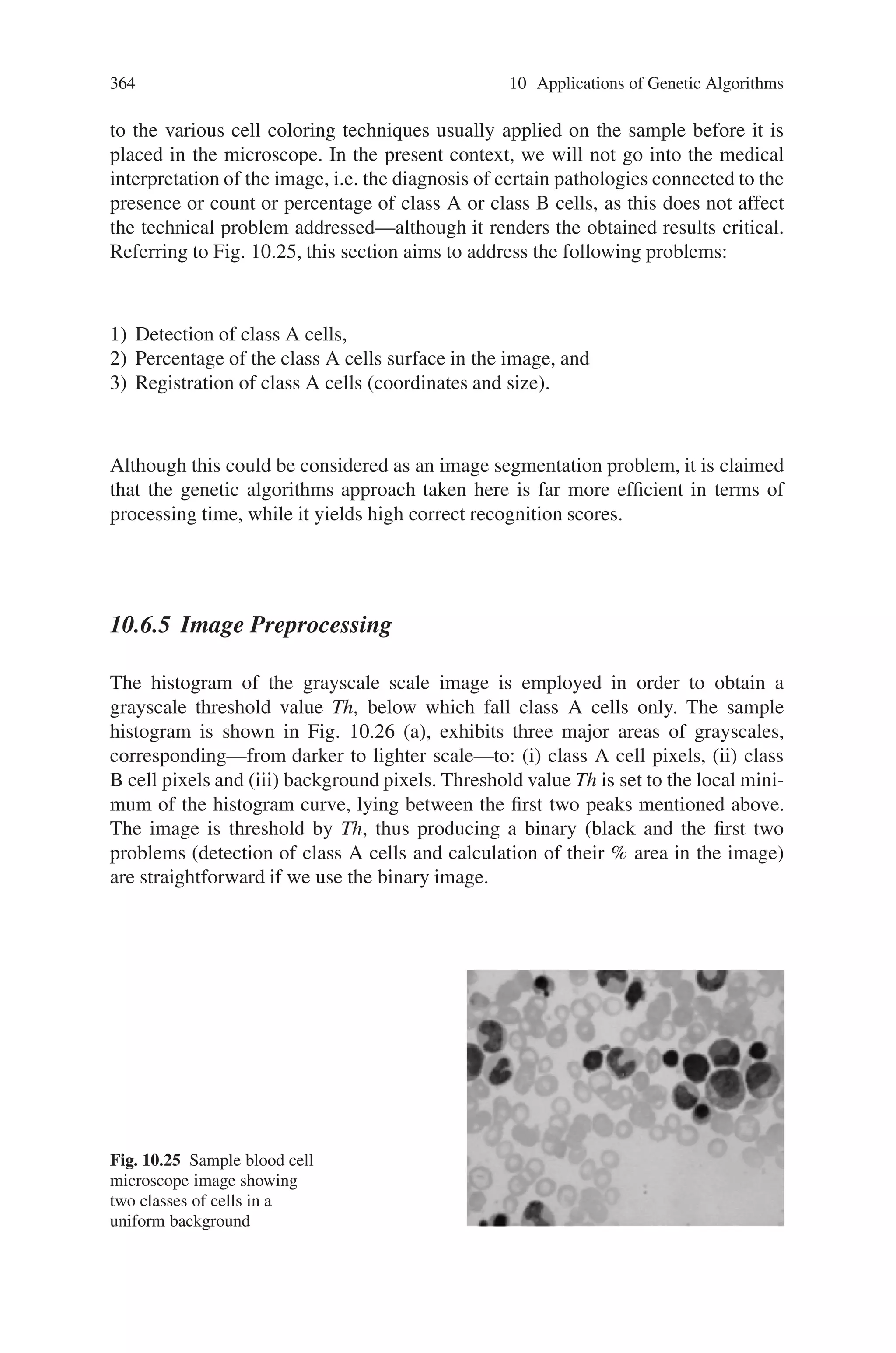
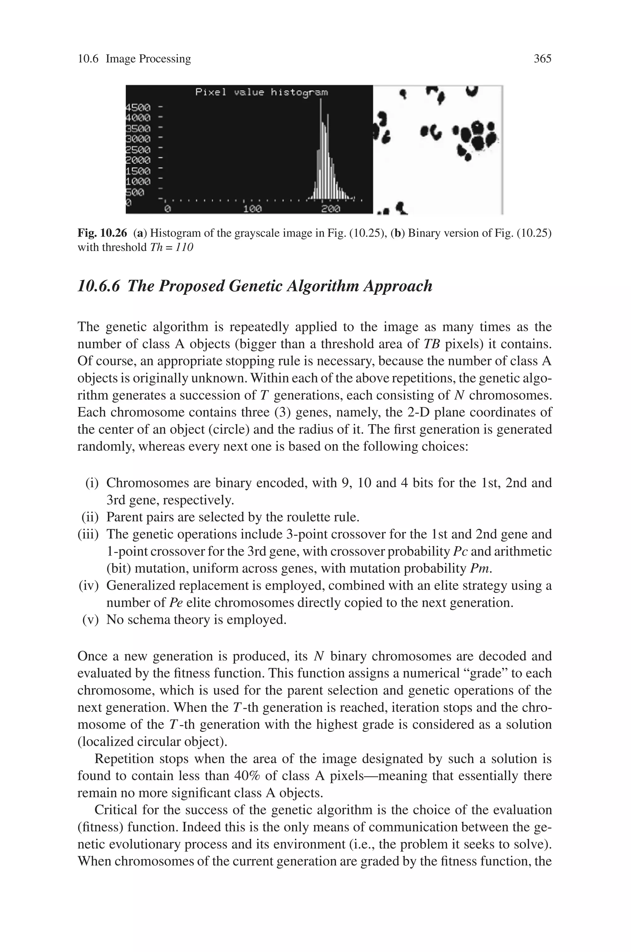
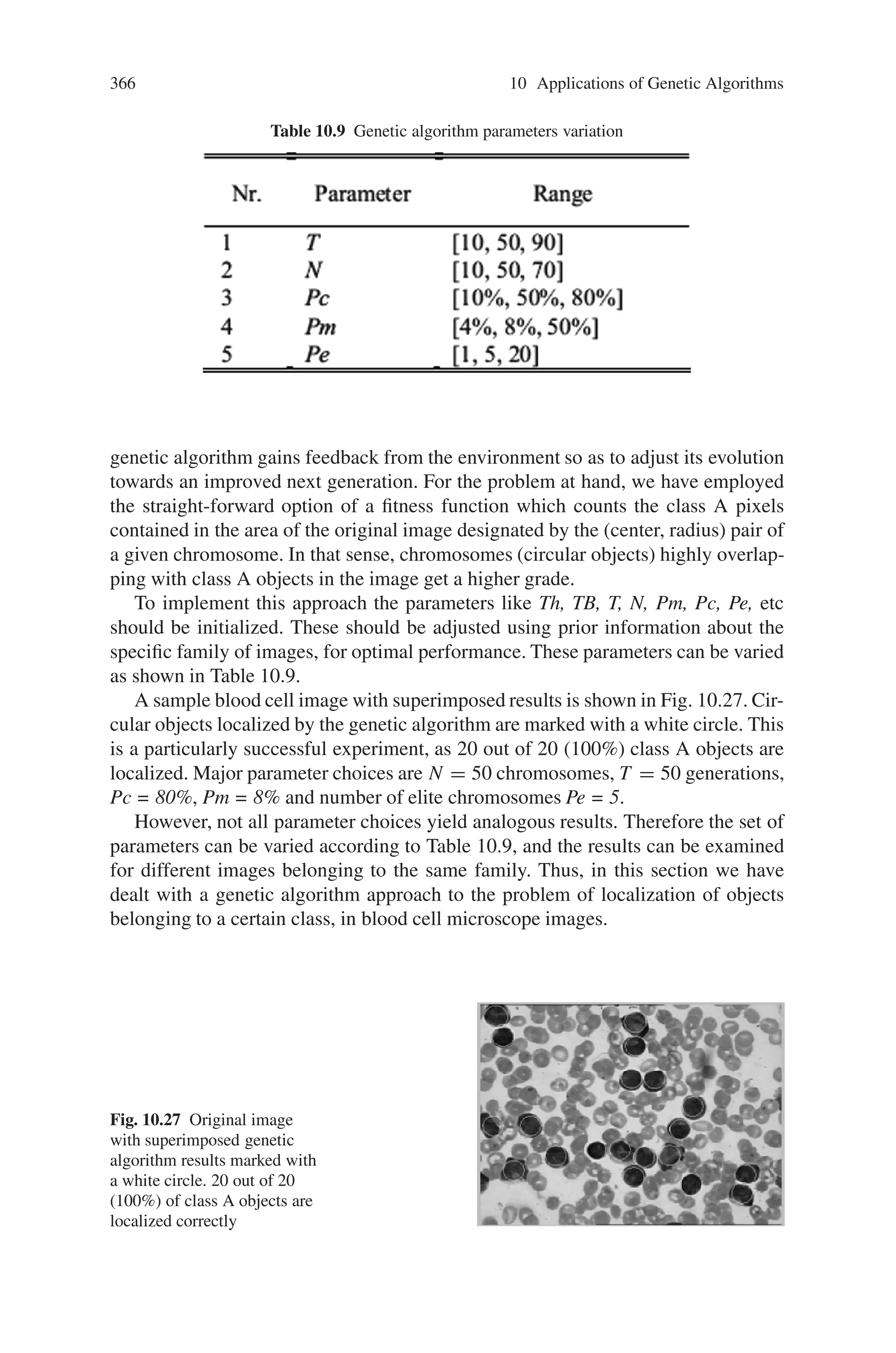
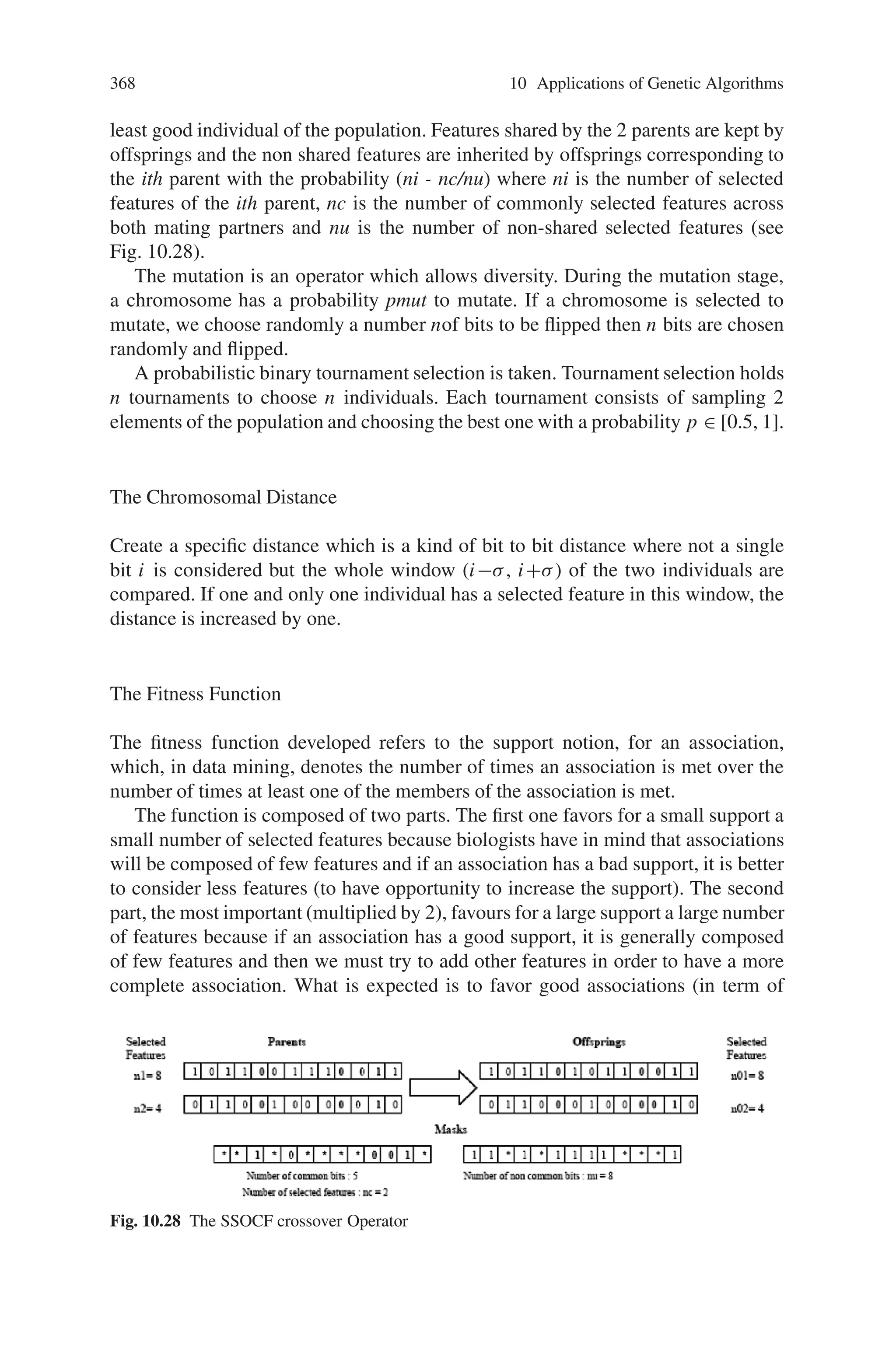
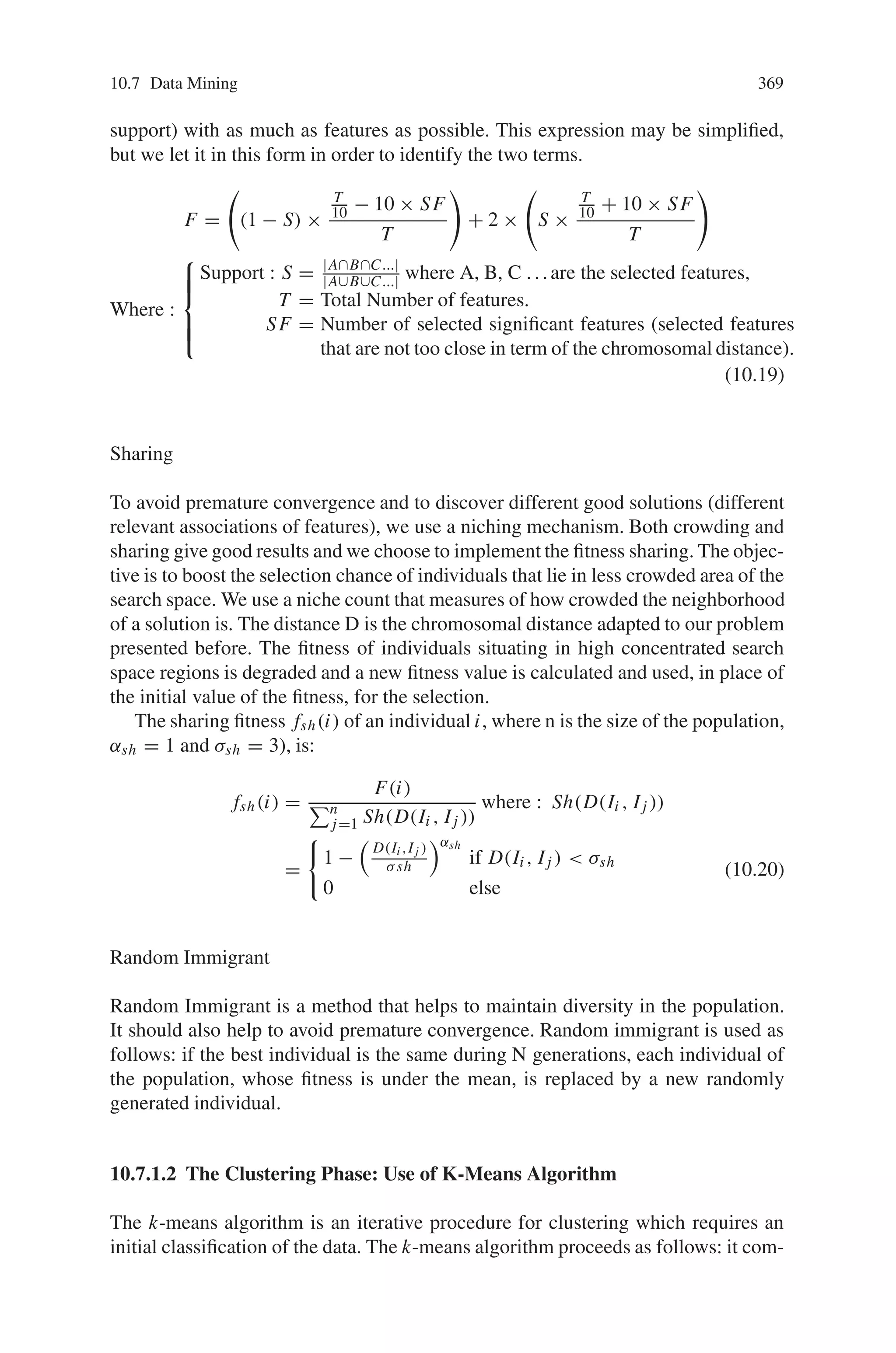
![368 10 Applications of Genetic Algorithms
least good individual of the population. Features shared by the 2 parents are kept by
offsprings and the non shared features are inherited by offsprings corresponding to
the ith parent with the probability (ni - nc/nu) where ni is the number of selected
features of the ith parent, nc is the number of commonly selected features across
both mating partners and nu is the number of non-shared selected features (see
Fig. 10.28).
The mutation is an operator which allows diversity. During the mutation stage,
a chromosome has a probability pmut to mutate. If a chromosome is selected to
mutate, we choose randomly a number nof bits to be flipped then n bits are chosen
randomly and flipped.
A probabilistic binary tournament selection is taken. Tournament selection holds
n tournaments to choose n individuals. Each tournament consists of sampling 2
elements of the population and choosing the best one with a probability p ∈ [0.5, 1].
The Chromosomal Distance
Create a specific distance which is a kind of bit to bit distance where not a single
bit i is considered but the whole window (i−σ, i+σ) of the two individuals are
compared. If one and only one individual has a selected feature in this window, the
distance is increased by one.
The Fitness Function
The fitness function developed refers to the support notion, for an association,
which, in data mining, denotes the number of times an association is met over the
number of times at least one of the members of the association is met.
The function is composed of two parts. The first one favors for a small support a
small number of selected features because biologists have in mind that associations
will be composed of few features and if an association has a bad support, it is better
to consider less features (to have opportunity to increase the support). The second
part, the most important (multiplied by 2), favours for a large support a large number
of features because if an association has a good support, it is generally composed
of few features and then we must try to add other features in order to have a more
complete association. What is expected is to favor good associations (in term of
Fig. 10.28 The SSOCF crossover Operator](https://image.slidesharecdn.com/s-220425101513/75/S-N-Sivanandam-S-N-Deepa-Introduction-to-Genetic-Algorithms-2008-ISBN-3540731894-pdf-381-2048.jpg)
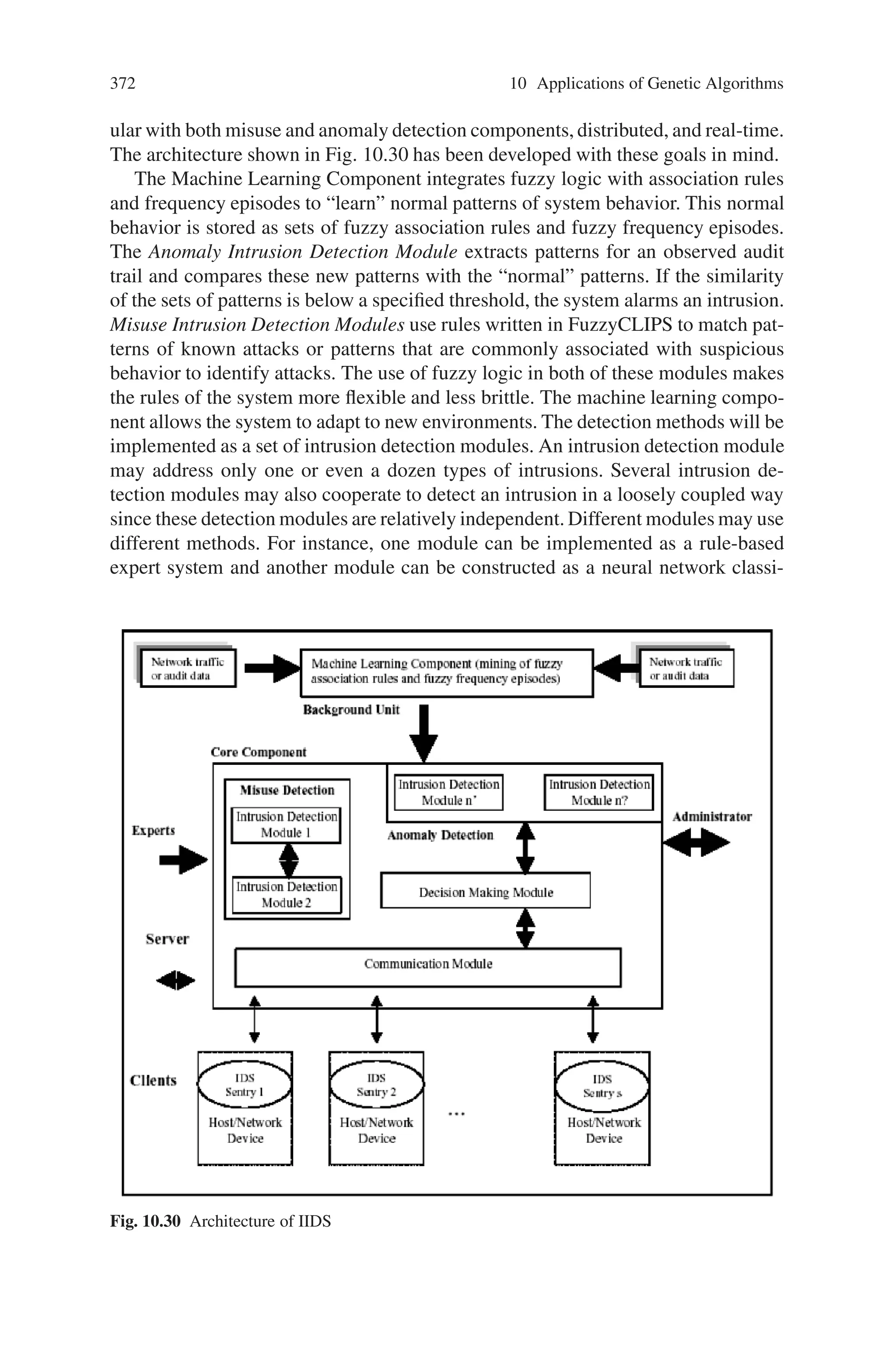
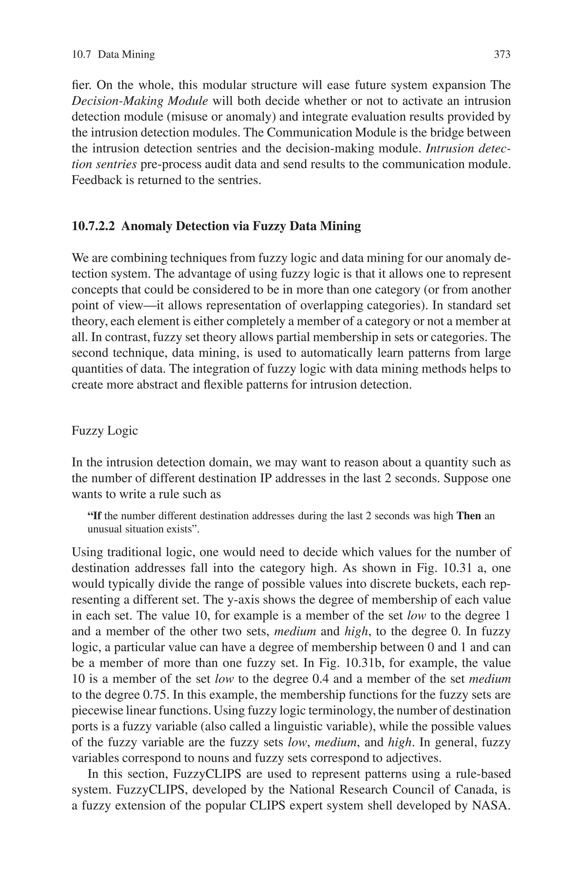
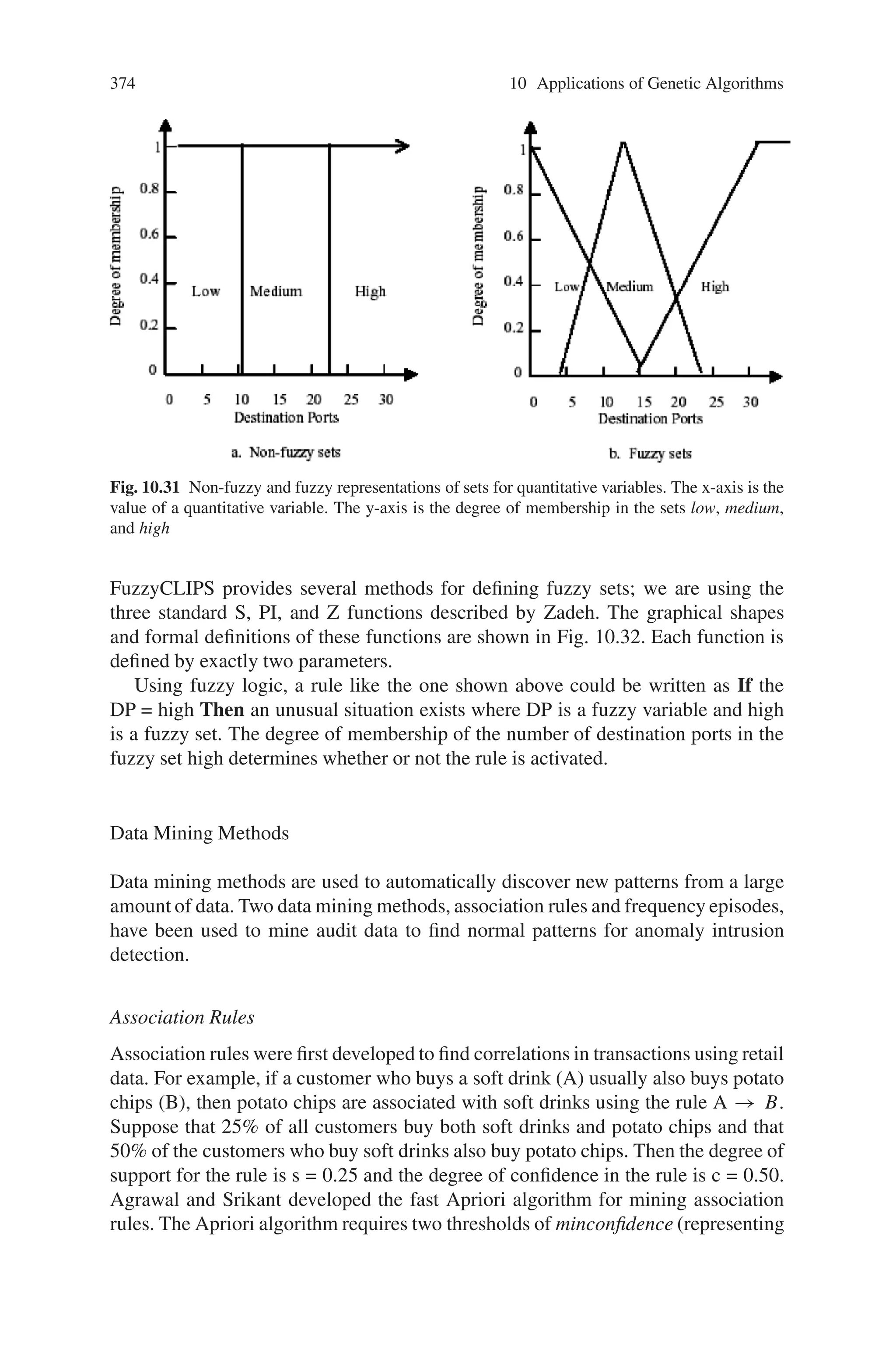
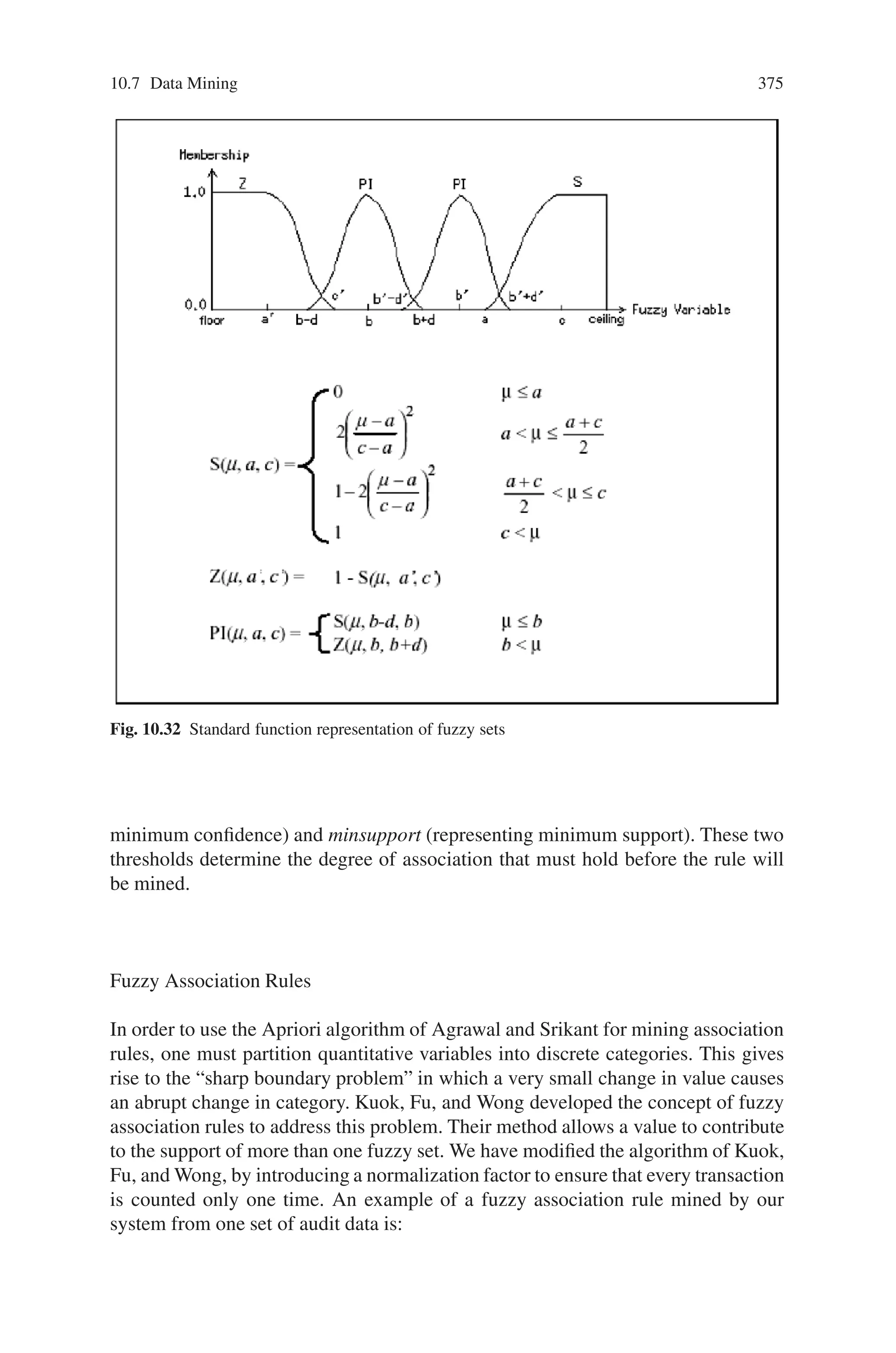
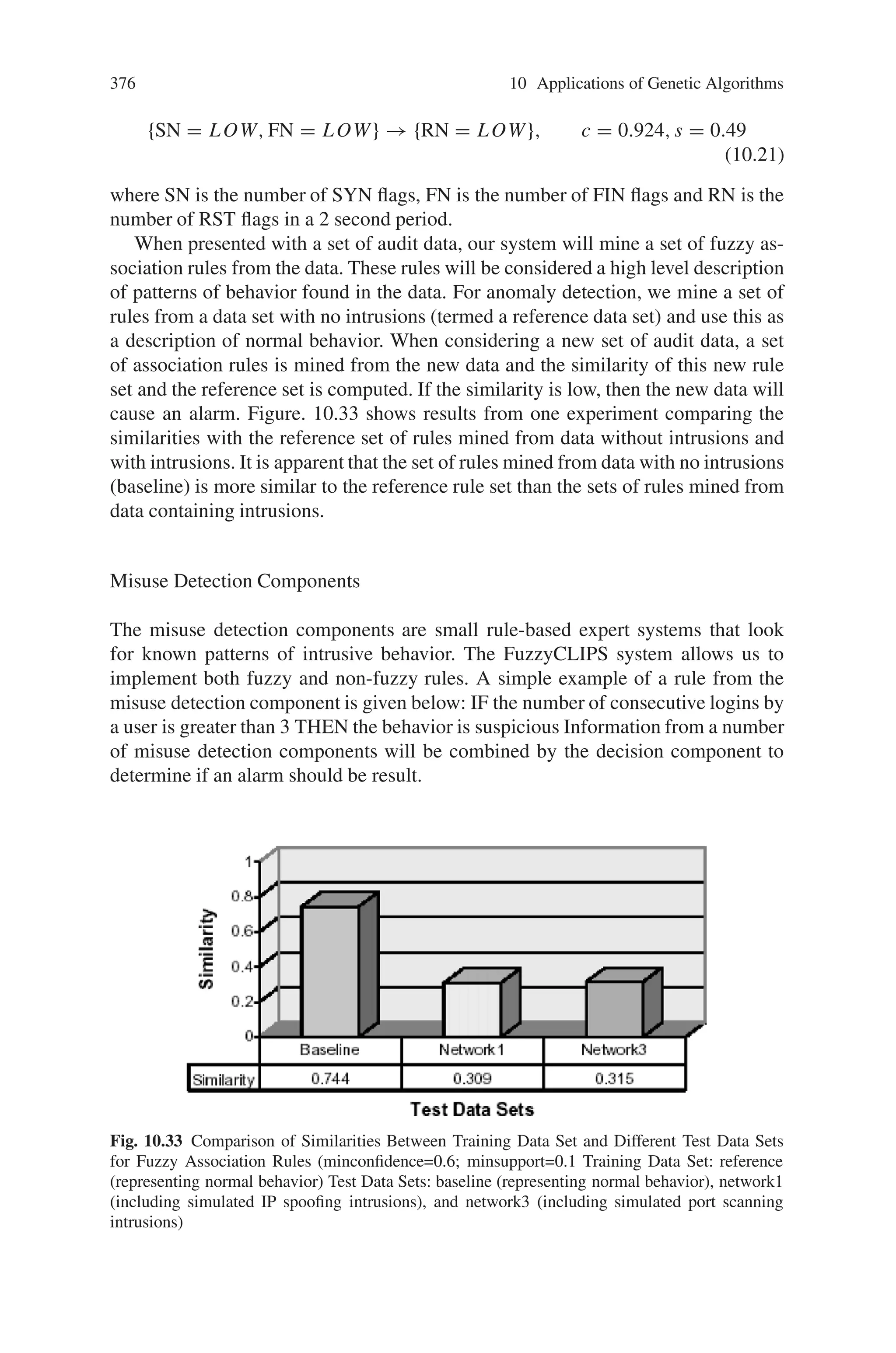
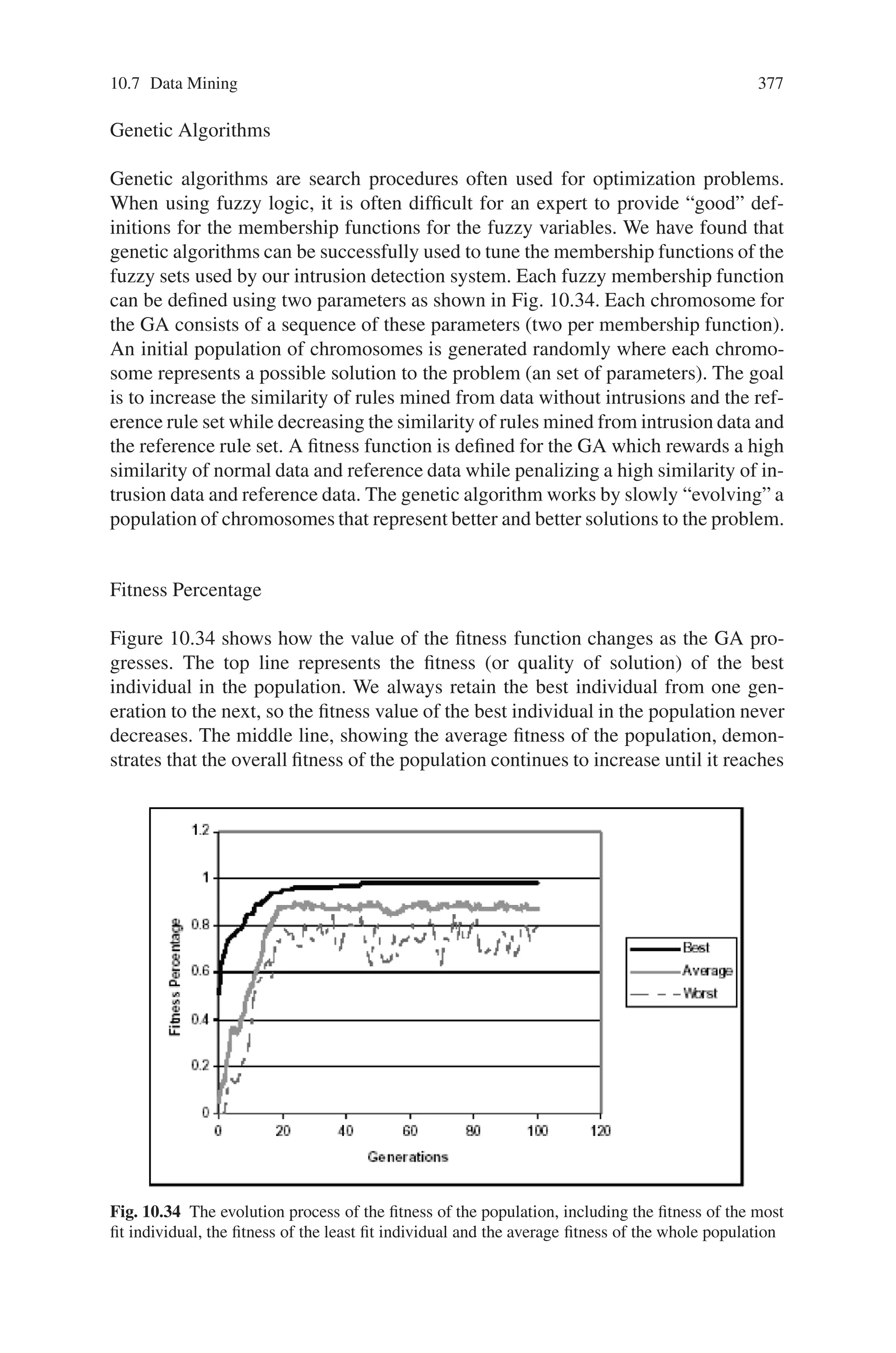
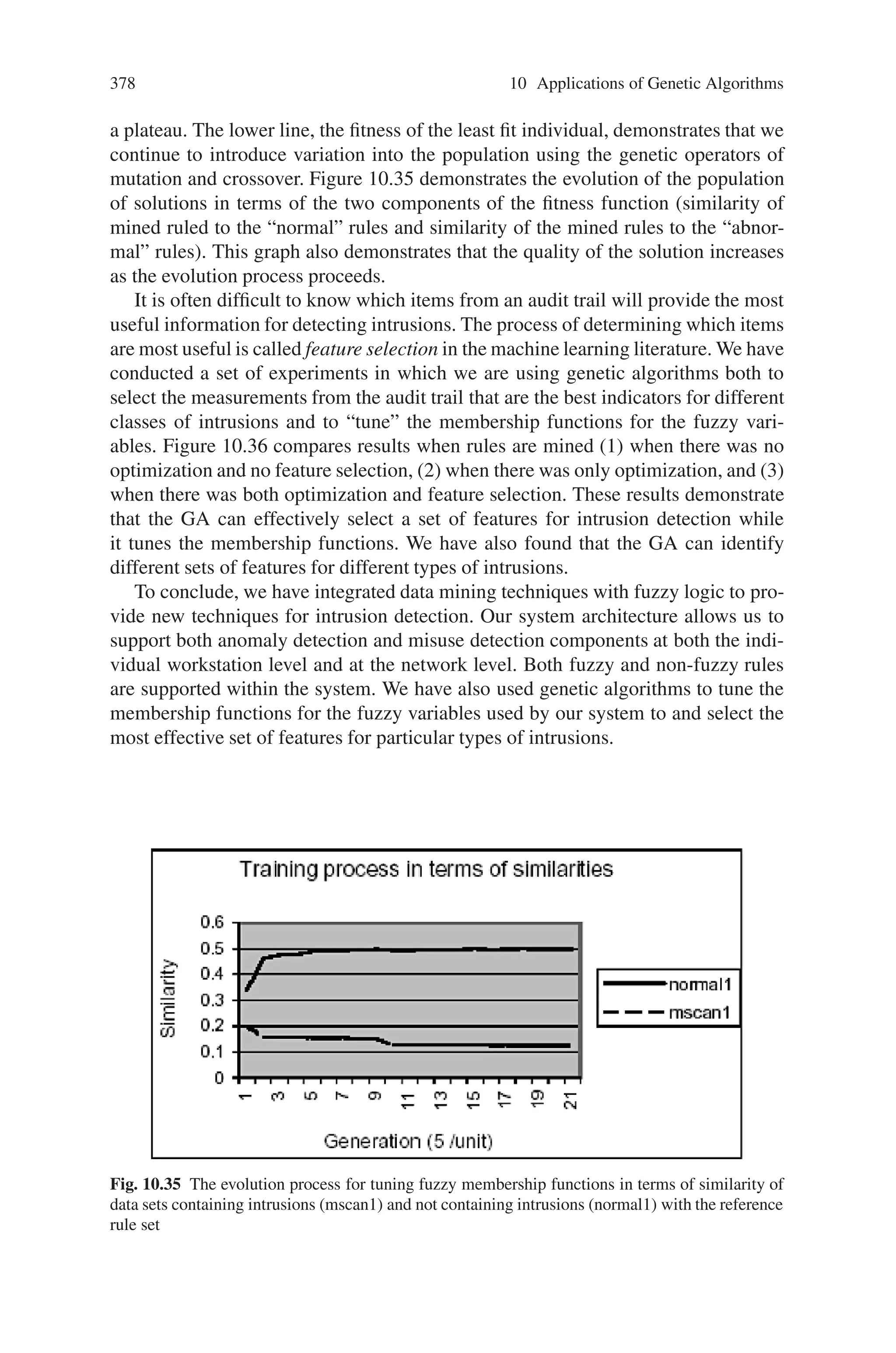
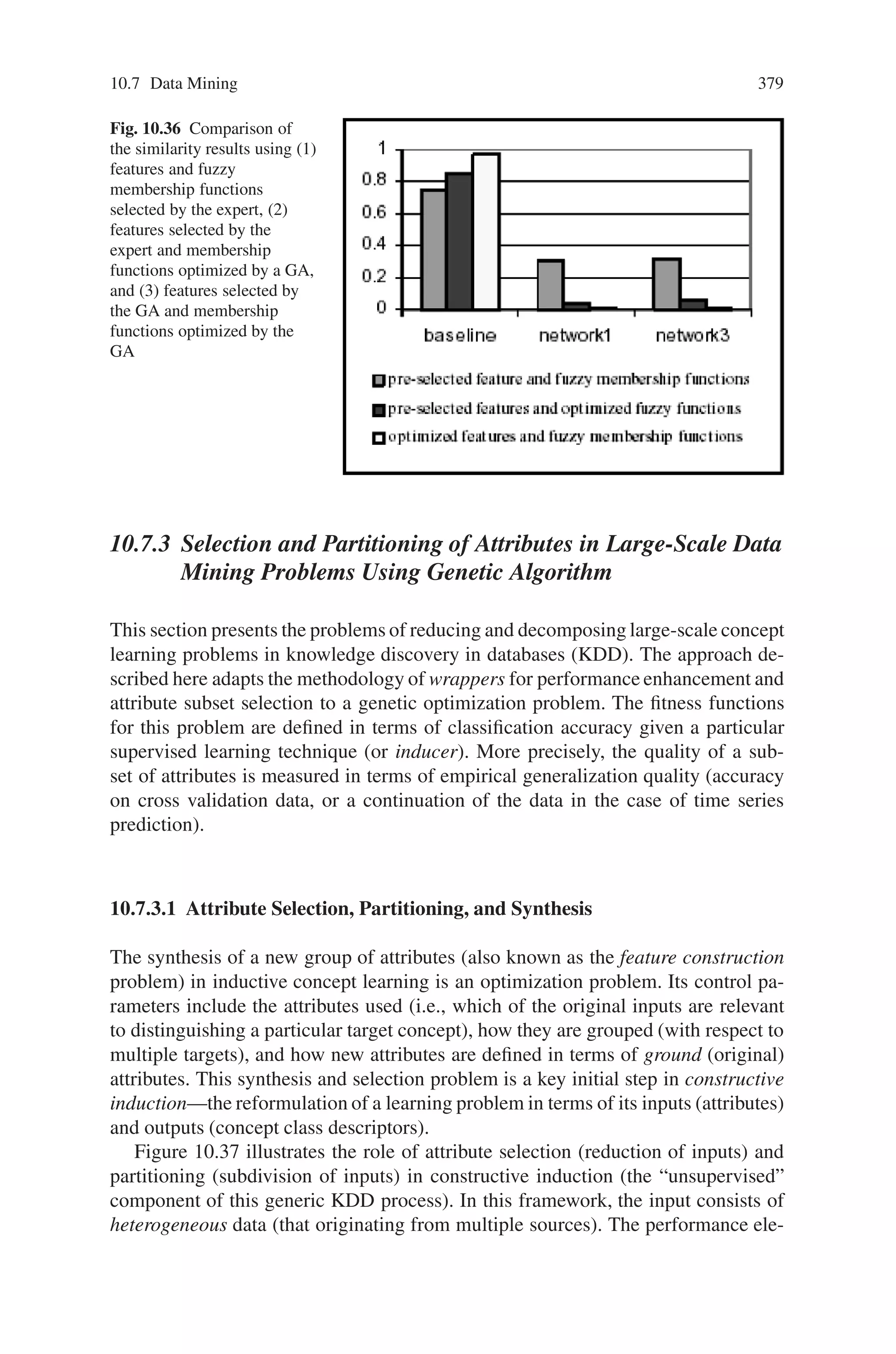
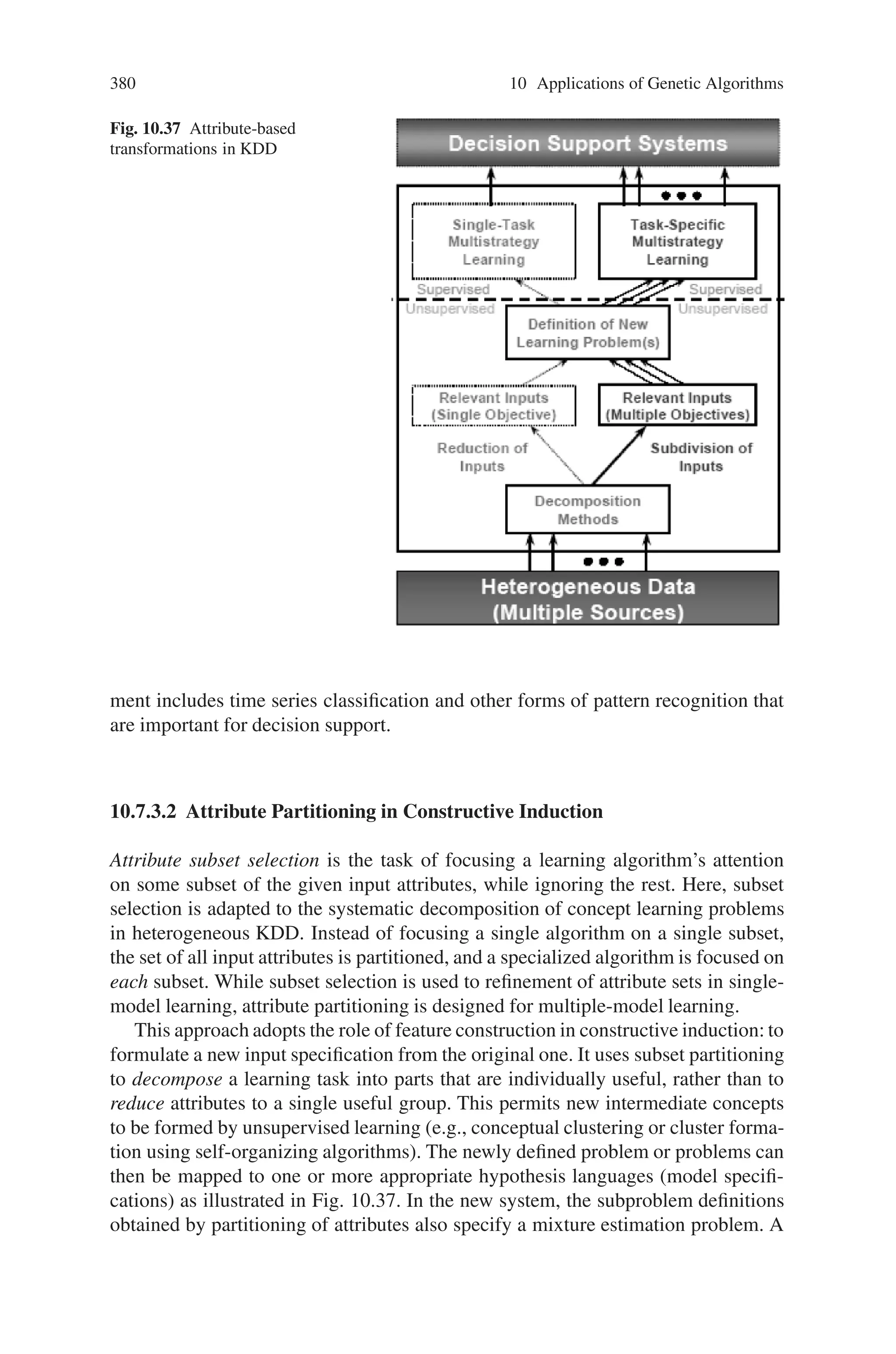
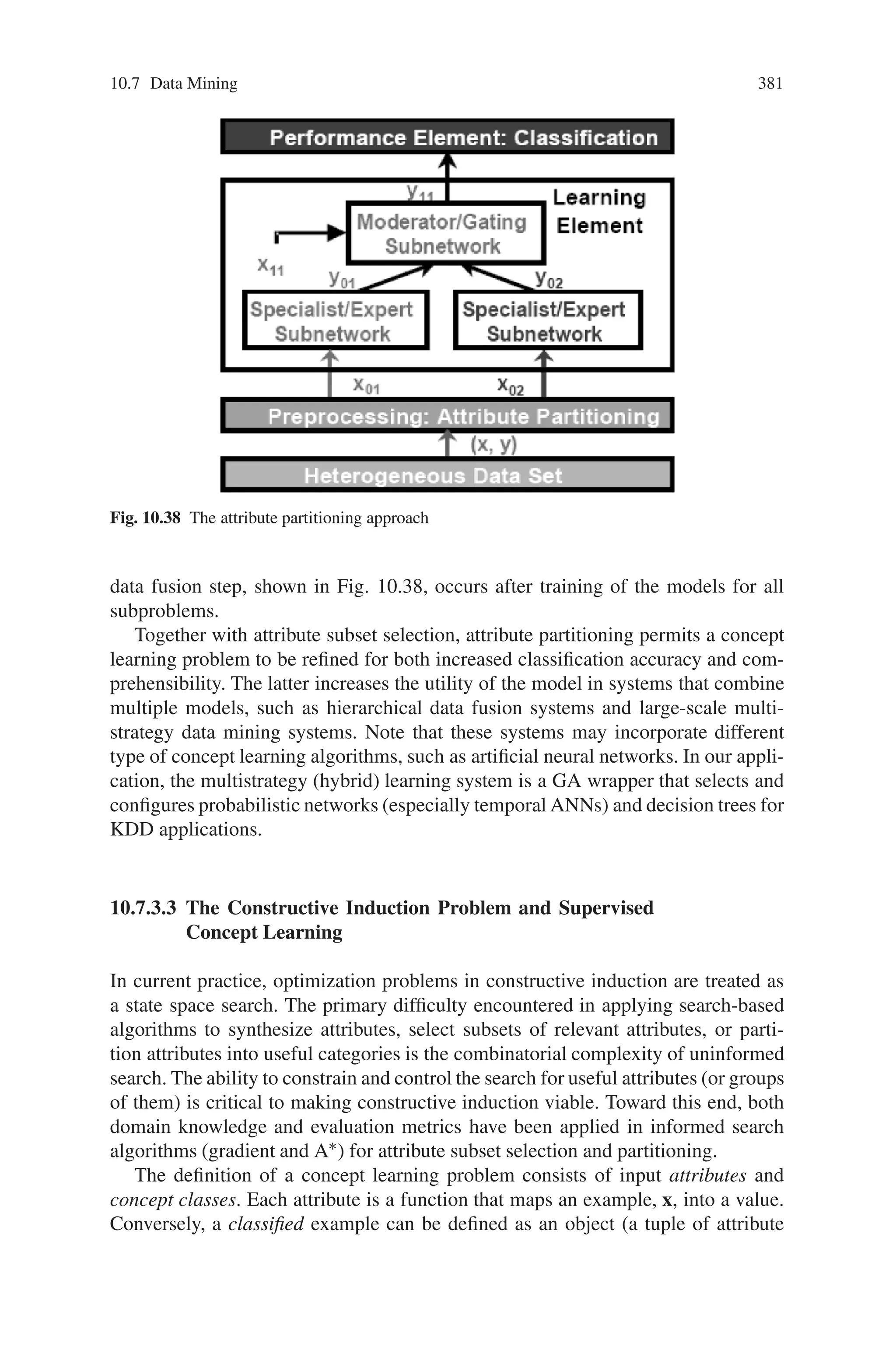
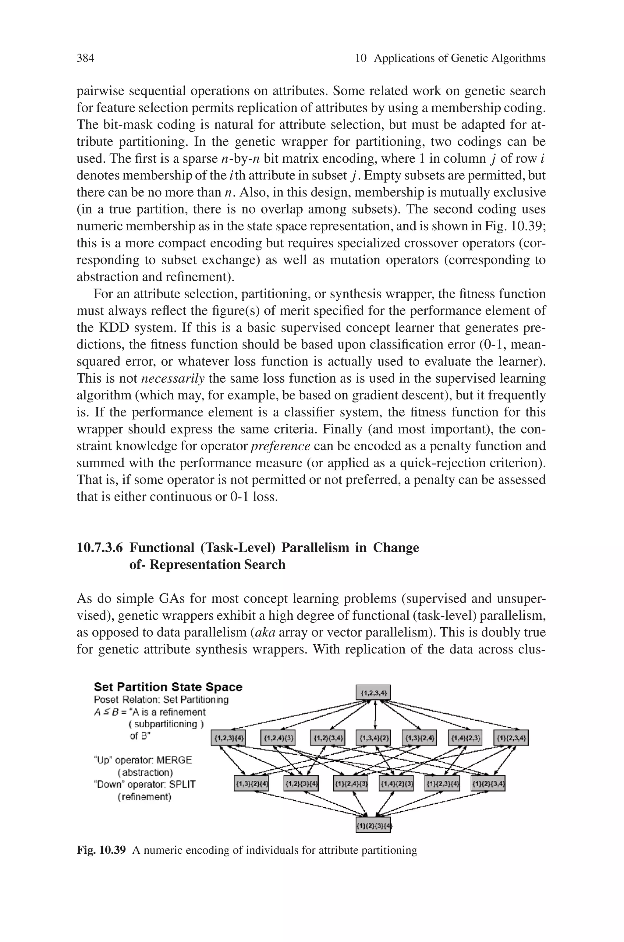
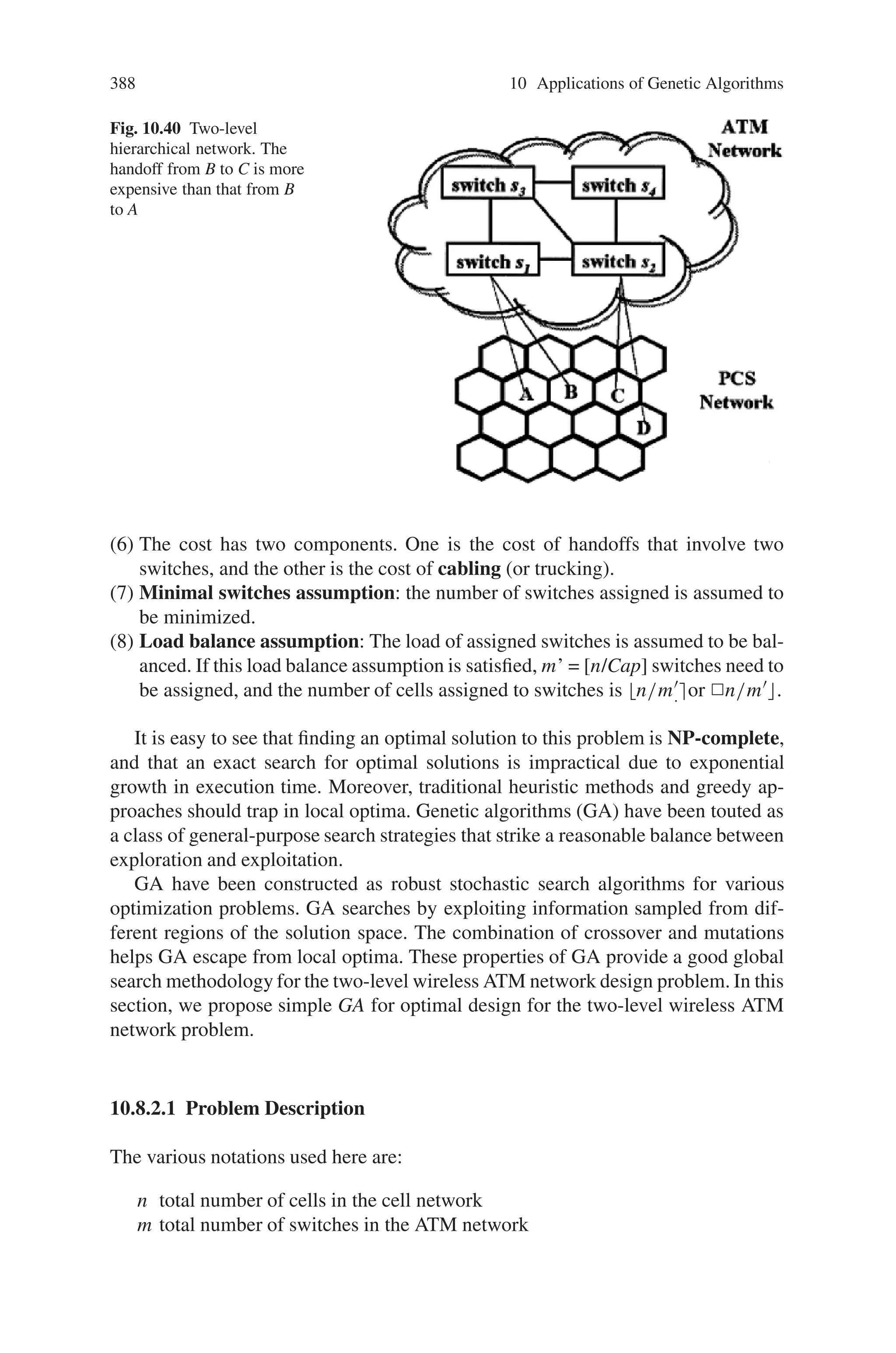
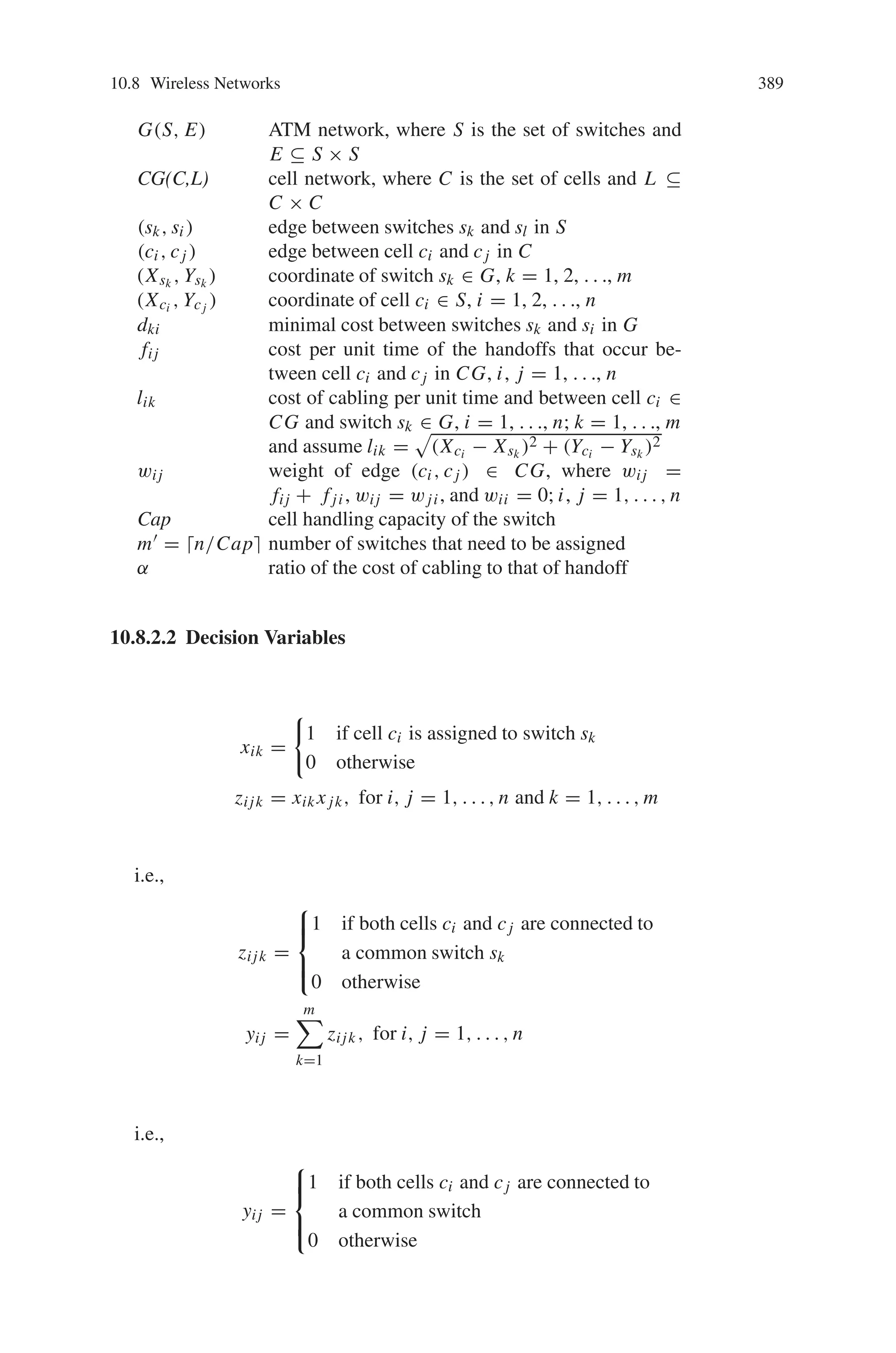
![388 10 Applications of Genetic Algorithms
Fig. 10.40 Two-level
hierarchical network. The
handoff from B to C is more
expensive than that from B
to A
(6) The cost has two components. One is the cost of handoffs that involve two
switches, and the other is the cost of cabling (or trucking).
(7) Minimal switches assumption: the number of switches assigned is assumed to
be minimized.
(8) Load balance assumption: The load of assigned switches is assumed to be bal-
anced. If this load balance assumption is satisfied, m’ = [n/Cap] switches need to
be assigned, and the number of cells assigned to switches is n/m
.or 2n/m.
It is easy to see that finding an optimal solution to this problem is NP-complete,
and that an exact search for optimal solutions is impractical due to exponential
growth in execution time. Moreover, traditional heuristic methods and greedy ap-
proaches should trap in local optima. Genetic algorithms (GA) have been touted as
a class of general-purpose search strategies that strike a reasonable balance between
exploration and exploitation.
GA have been constructed as robust stochastic search algorithms for various
optimization problems. GA searches by exploiting information sampled from dif-
ferent regions of the solution space. The combination of crossover and mutations
helps GA escape from local optima. These properties of GA provide a good global
search methodology for the two-level wireless ATM network design problem. In this
section, we propose simple GA for optimal design for the two-level wireless ATM
network problem.
10.8.2.1 Problem Description
The various notations used here are:
n total number of cells in the cell network
m total number of switches in the ATM network](https://image.slidesharecdn.com/s-220425101513/75/S-N-Sivanandam-S-N-Deepa-Introduction-to-Genetic-Algorithms-2008-ISBN-3540731894-pdf-401-2048.jpg)
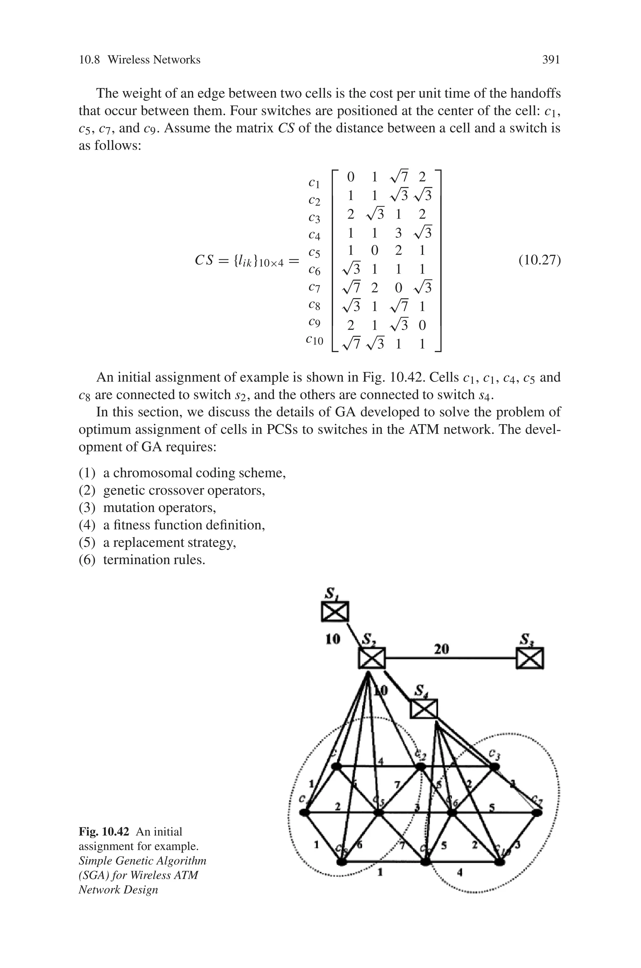
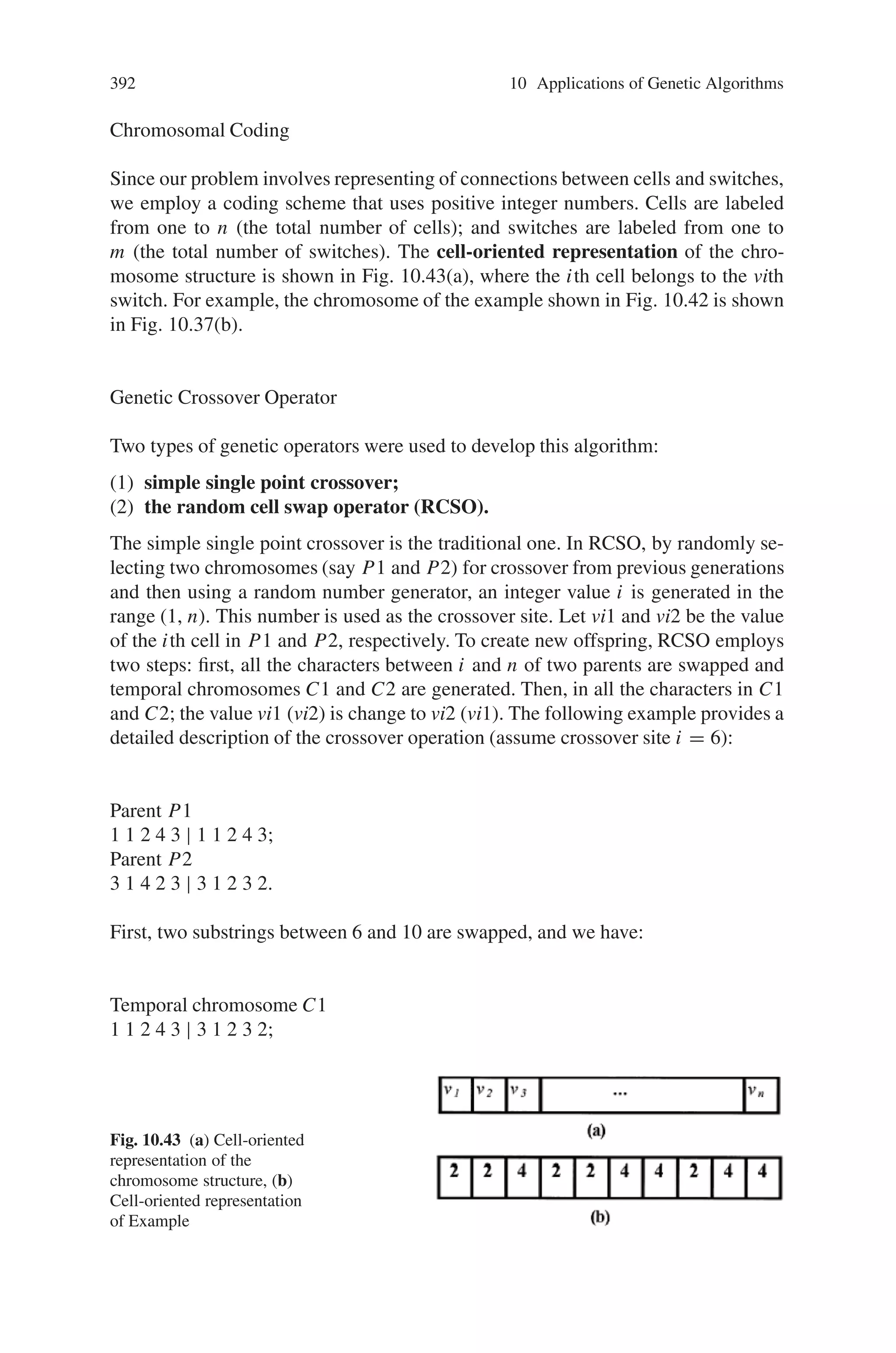
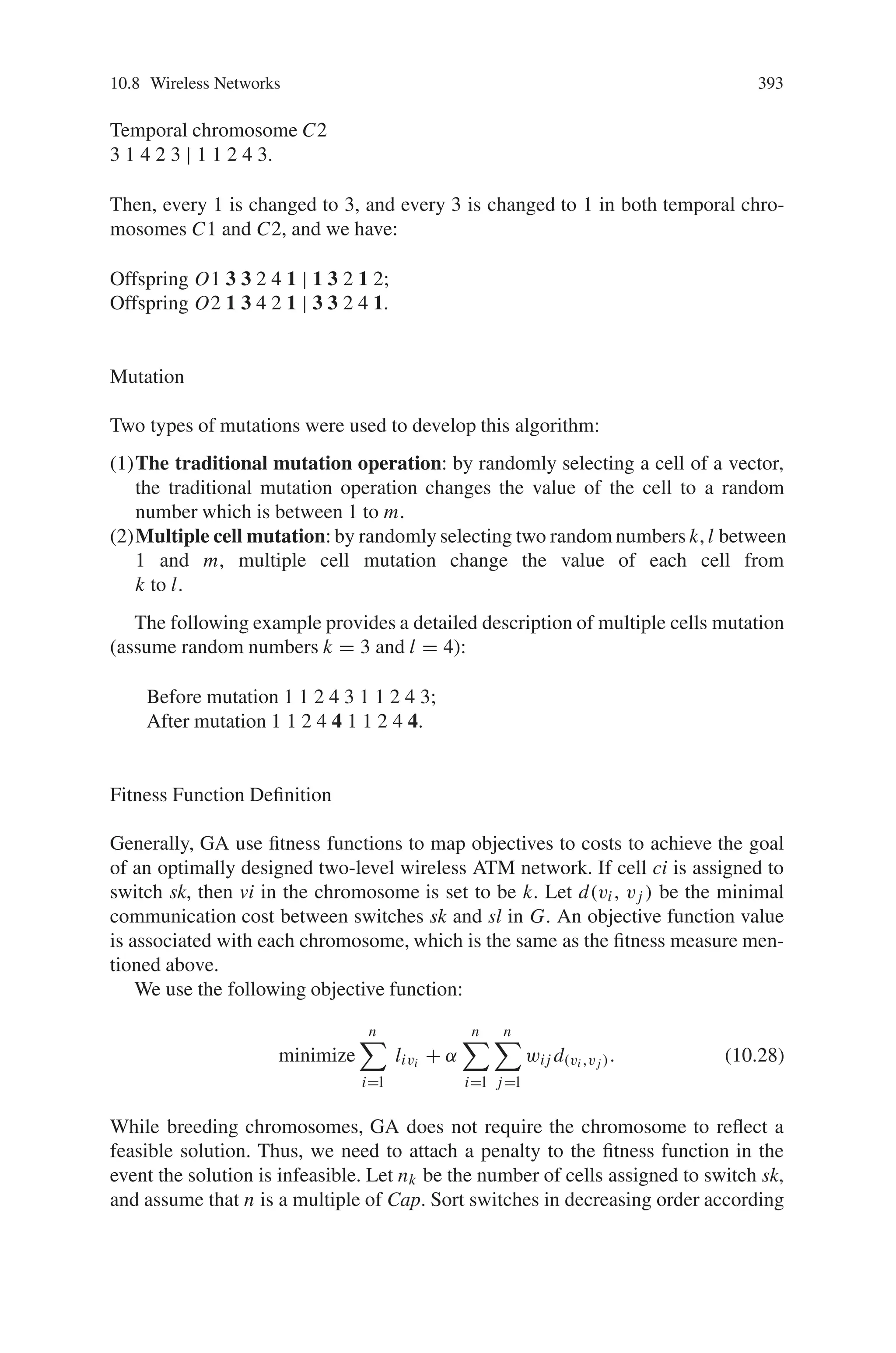
![394 10 Applications of Genetic Algorithms
to the number of cells to be assigned. We rewrite the formulation above in an
unconstrained form:
minimize cost =
n
i=l
livi + α
n
i=l
n
j=l
wij d(vi,vj ) + Π,
where
Π = β(
m
k=1
|nk − Cap| +
m
k=m+1
|nk|). (10.29)
%
is the penalty measure associated with a chromosome, and β is the penalty
weight.
Since the best-fit chromosomes should have a probability of being selected as
parents that is proportional to their fitness, they need to be expressed in a maxi-
mization form. This is done by subtracting the objective from a large number Cmax.
Hence, the fitness function becomes:
maximize Cmax − [
n
i=l
livi + α
n
i=l
n
j=l
wij d(vi,vj )
+ β(
m
k=1
|nk − Cap| +
m
k=m+1
|nk|)],
(10.30)
where Cmax denotes the maximum value observed, so far, of the cost function in the
population. Let cost be the value of the cost function for the chromosome; Cmax can
be calculated by the following iterative equation:
Cmax = max {Cmax, cost}, (10.31)
where Cmax is initialized to zero.
Replacement Strategy
This subsection discusses a method used to create a new generation after crossover
and mutation is carried out on the chromosomes of the previous generation. The
most common strategies probabilistically replace the poorest performing chromo-
somes in the previous generation. The elitist strategy appends the best performing
chromosome of a previous generation to the current population and thereby ensures
that the chromosome with the best objective function value always survives to the
next generation. The algorithm developed here combines both the concepts main-
tained above.](https://image.slidesharecdn.com/s-220425101513/75/S-N-Sivanandam-S-N-Deepa-Introduction-to-Genetic-Algorithms-2008-ISBN-3540731894-pdf-407-2048.jpg)
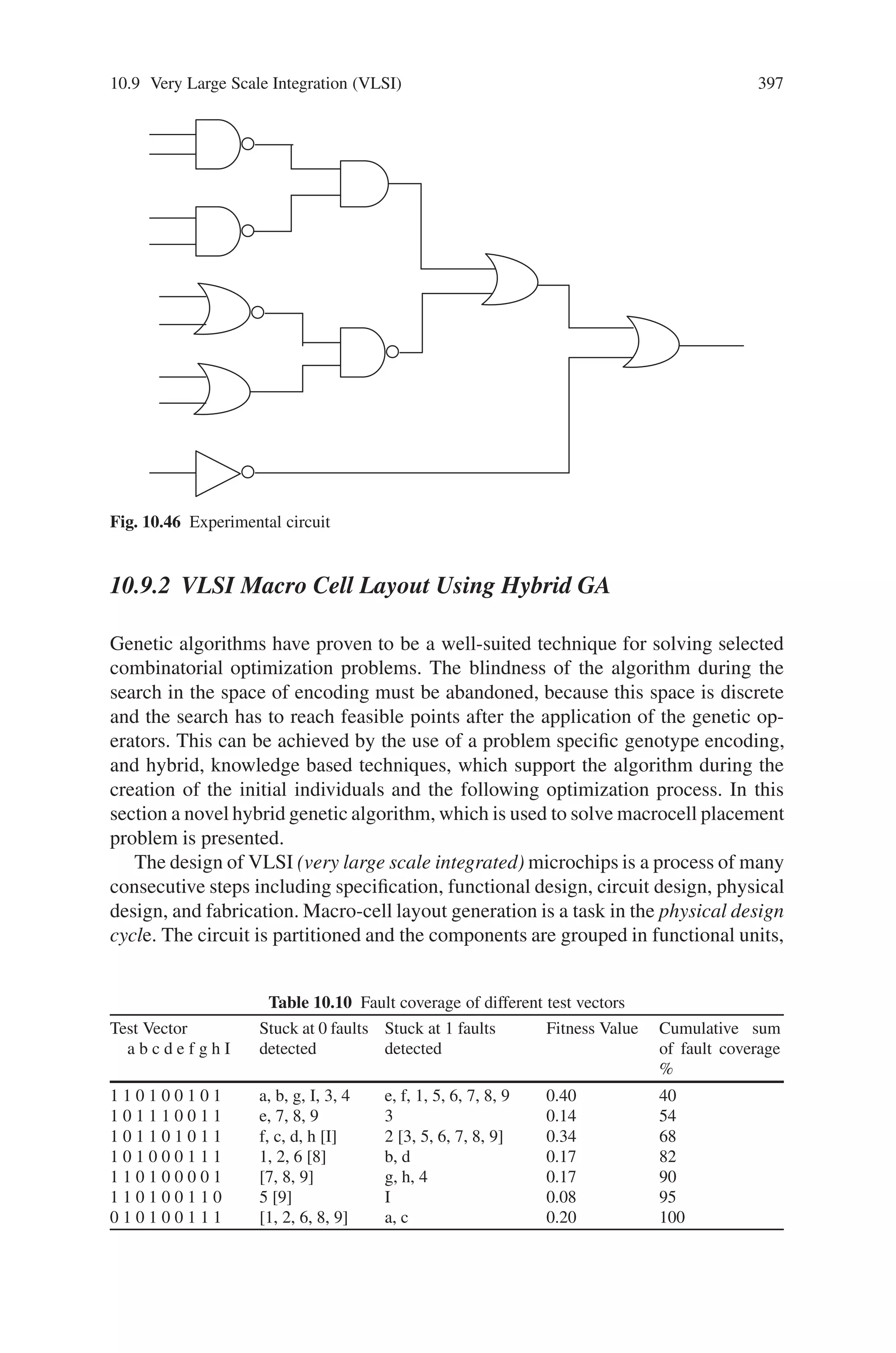
![396 10 Applications of Genetic Algorithms
Digital Circuit
Comparator
Input Test Patterns
Stored Correct response
Fig. 10.44 Digital circuit
• Test vectors are encoded as Binary bit stream.
• Fitness function gives the number of faults covered by each test vector.
Consider the XOR circuit shown in the Fig. 10.45 below.
The description of given XOR Circuit is as follows:
• Number of primary inputs is “2” and primary output is “1”.
• Each parent width is 2 bits.
• In this example, XOR circuit has 12 fault sites and 24 stuck at faults.
• For a fault free circuit, the output is “1” for a input vector [1,0].
• If the circuit has a stuck at “0” at “a”, the output response is “0”. So input vector
[1,0] detects stuck at 0 [SA0] fault at “a”.
• Like wise [1,0] can also detect SA0 fault at [a, c, d, g, h, z] and SA1 at [b, e, j].
• Thus [1,0] can detect 9 out of a total of 24 faults and it’s fitness is 0.375
[i.e. 9/24].
The experimental circuit is as given below in Fig. 10.46. Table 10.10 shows the
fault coverage of different test vectors.
The advantages of GA in VLSI Testing is as follows:
• Concept is easy to understand and separate from the application.
• Easy to exploit previous or alternate solutions.
• They are adaptive and learn from experience.
• They are efficient for complex programs.
• They are easy to parallelize as they have intrinsic parallelism.
• As they are inherently parallel, the computation can be easily distributed.
a h j
g
i
k
b
1
0 z
Fig. 10.45 XOR circuit](https://image.slidesharecdn.com/s-220425101513/75/S-N-Sivanandam-S-N-Deepa-Introduction-to-Genetic-Algorithms-2008-ISBN-3540731894-pdf-409-2048.jpg)
![10.9 Very Large Scale Integration (VLSI) 397
Fig. 10.46 Experimental circuit
10.9.2 VLSI Macro Cell Layout Using Hybrid GA
Genetic algorithms have proven to be a well-suited technique for solving selected
combinatorial optimization problems. The blindness of the algorithm during the
search in the space of encoding must be abandoned, because this space is discrete
and the search has to reach feasible points after the application of the genetic op-
erators. This can be achieved by the use of a problem specific genotype encoding,
and hybrid, knowledge based techniques, which support the algorithm during the
creation of the initial individuals and the following optimization process. In this
section a novel hybrid genetic algorithm, which is used to solve macrocell placement
problem is presented.
The design of VLSI (very large scale integrated) microchips is a process of many
consecutive steps including specification, functional design, circuit design, physical
design, and fabrication. Macro-cell layout generation is a task in the physical design
cycle. The circuit is partitioned and the components are grouped in functional units,
Table 10.10 Fault coverage of different test vectors
Test Vector
a b c d e f g h I
Stuck at 0 faults
detected
Stuck at 1 faults
detected
Fitness Value Cumulative sum
of fault coverage
%
1 1 0 1 0 0 1 0 1 a, b, g, I, 3, 4 e, f, 1, 5, 6, 7, 8, 9 0.40 40
1 0 1 1 1 0 0 1 1 e, 7, 8, 9 3 0.14 54
1 0 1 1 0 1 0 1 1 f, c, d, h [I] 2 [3, 5, 6, 7, 8, 9] 0.34 68
1 0 1 0 0 0 1 1 1 1, 2, 6 [8] b, d 0.17 82
1 1 0 1 0 0 0 0 1 [7, 8, 9] g, h, 4 0.17 90
1 1 0 1 0 0 1 1 0 5 [9] I 0.08 95
0 1 0 1 0 0 1 1 1 [1, 2, 6, 8, 9] a, c 0.20 100](https://image.slidesharecdn.com/s-220425101513/75/S-N-Sivanandam-S-N-Deepa-Introduction-to-Genetic-Algorithms-2008-ISBN-3540731894-pdf-410-2048.jpg)

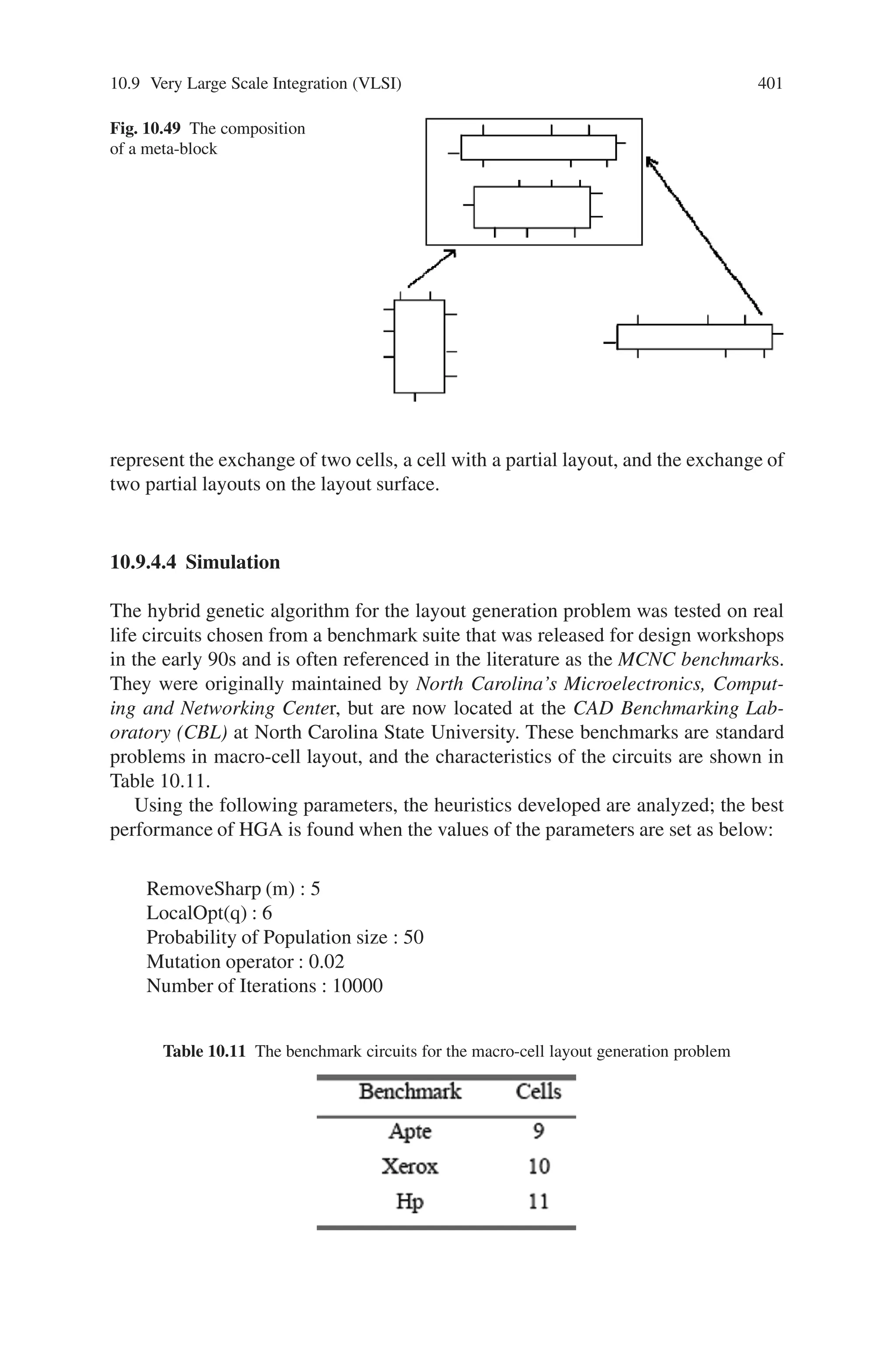
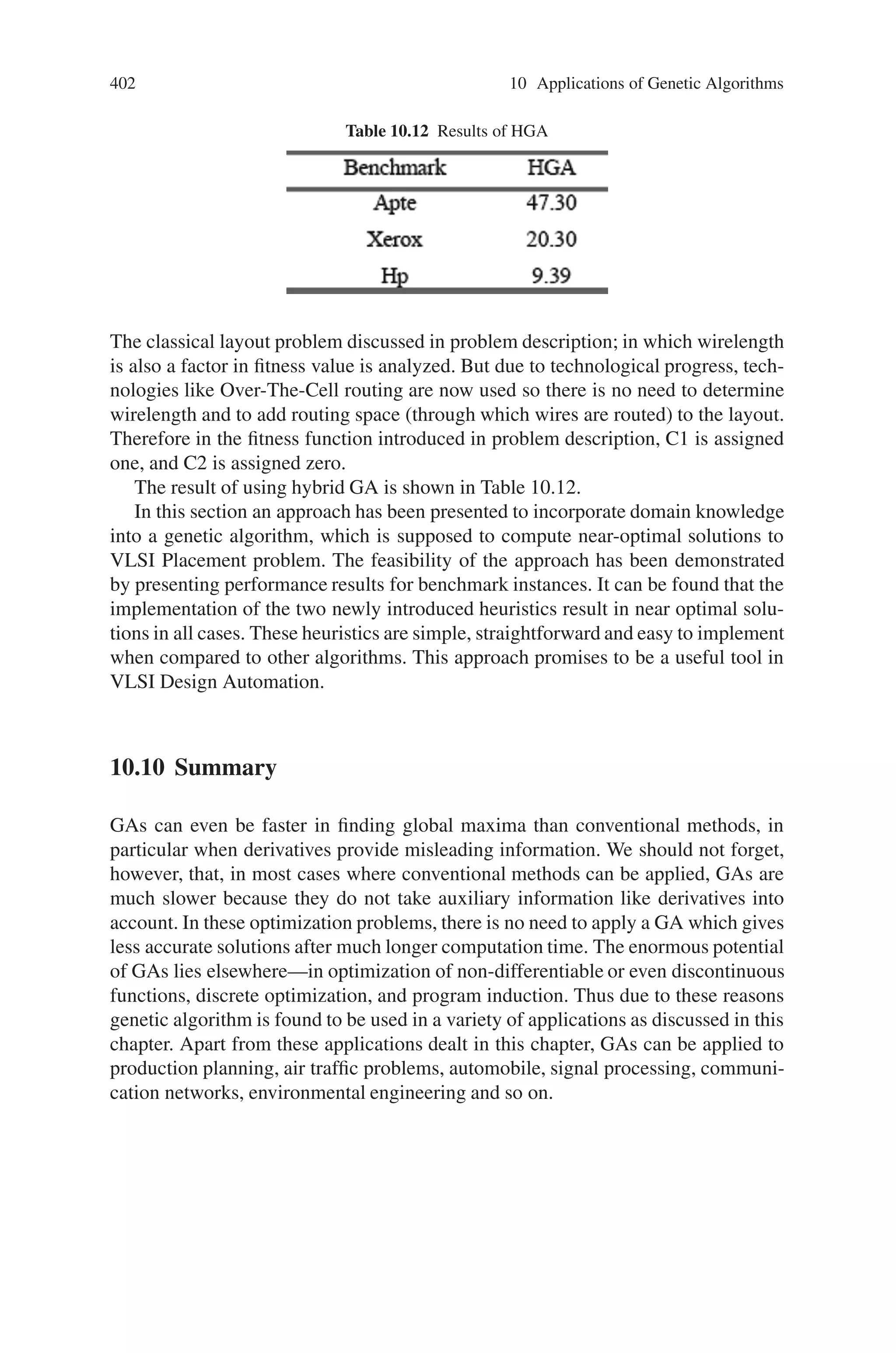
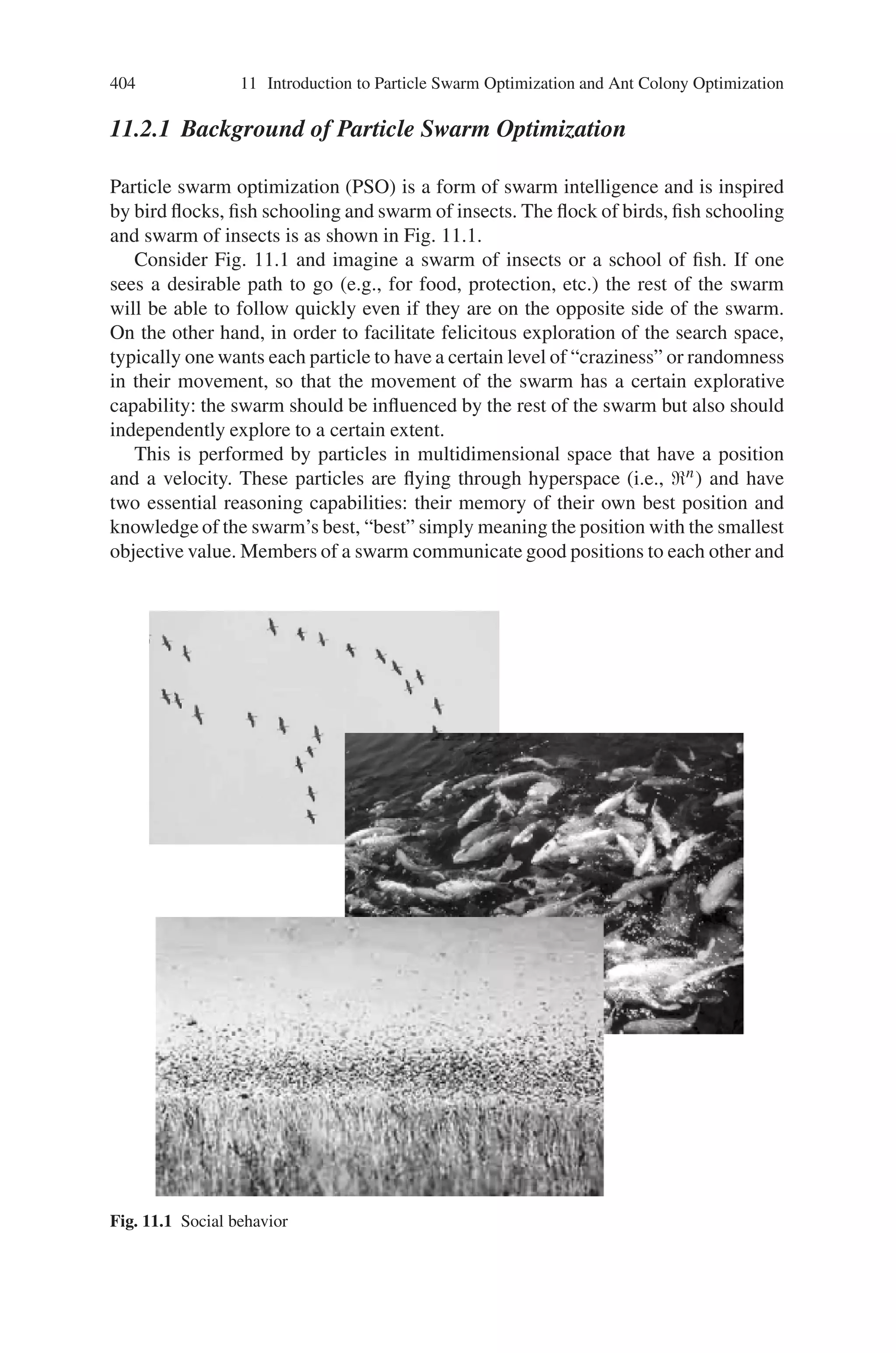
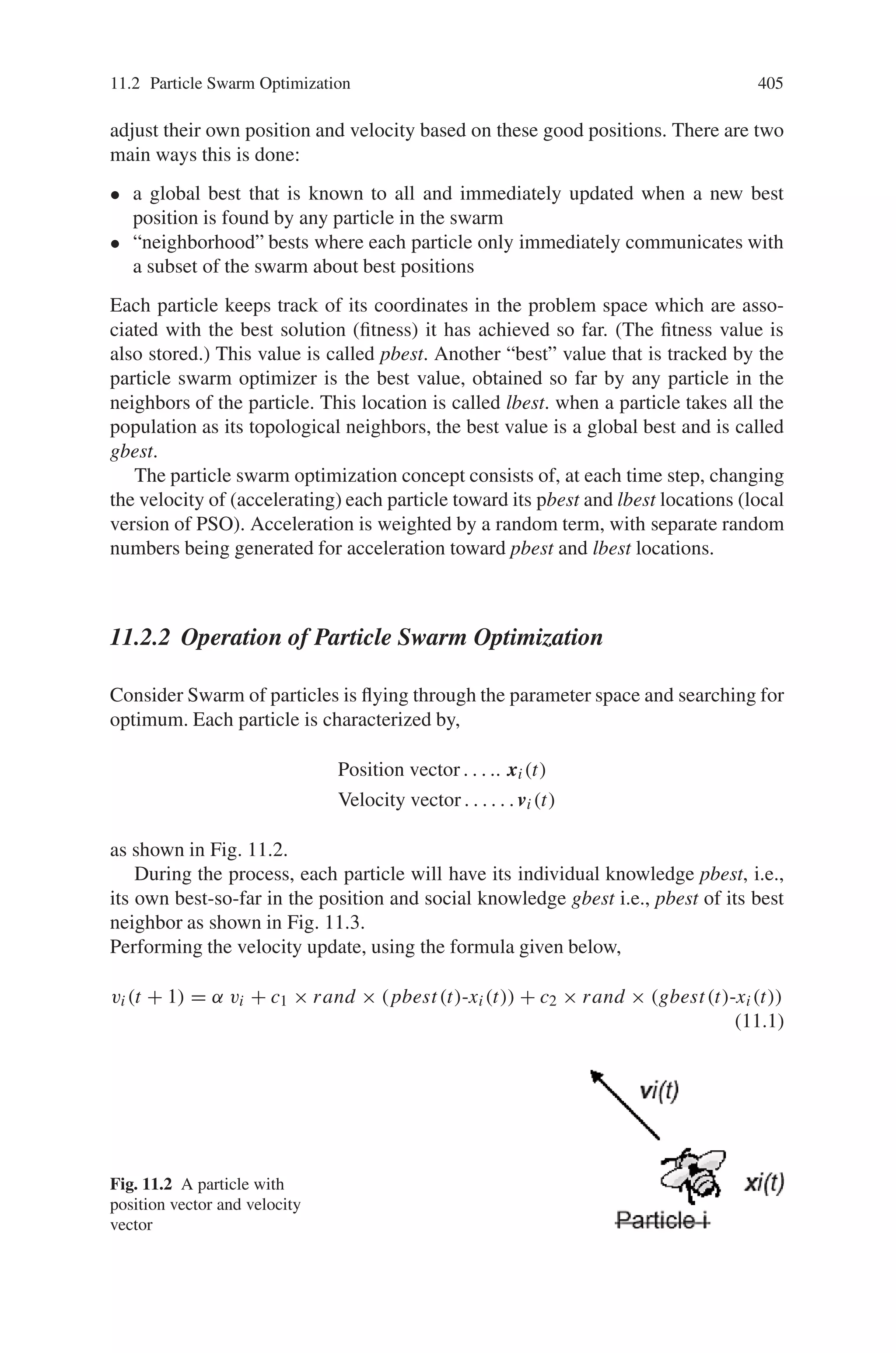
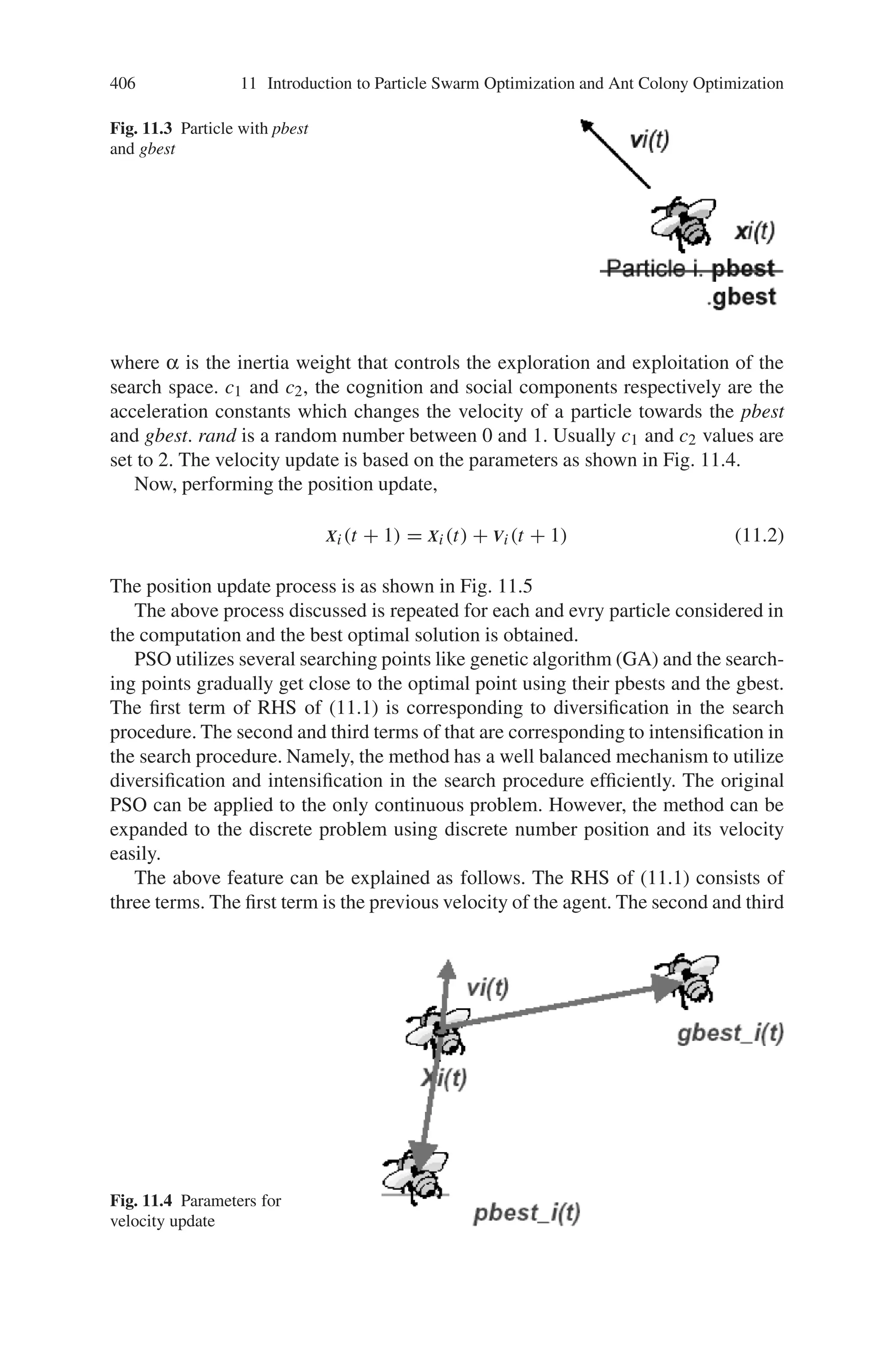
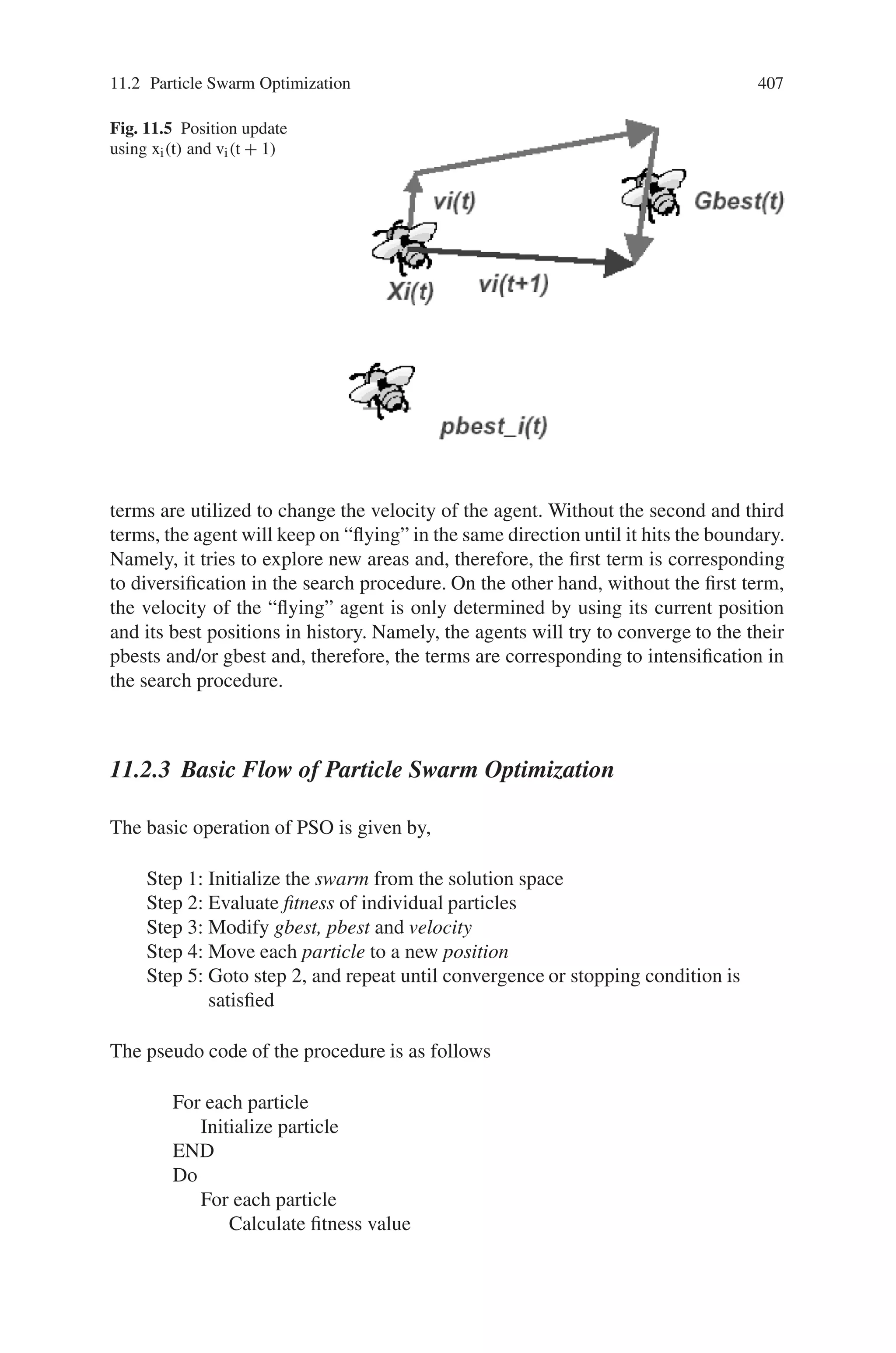
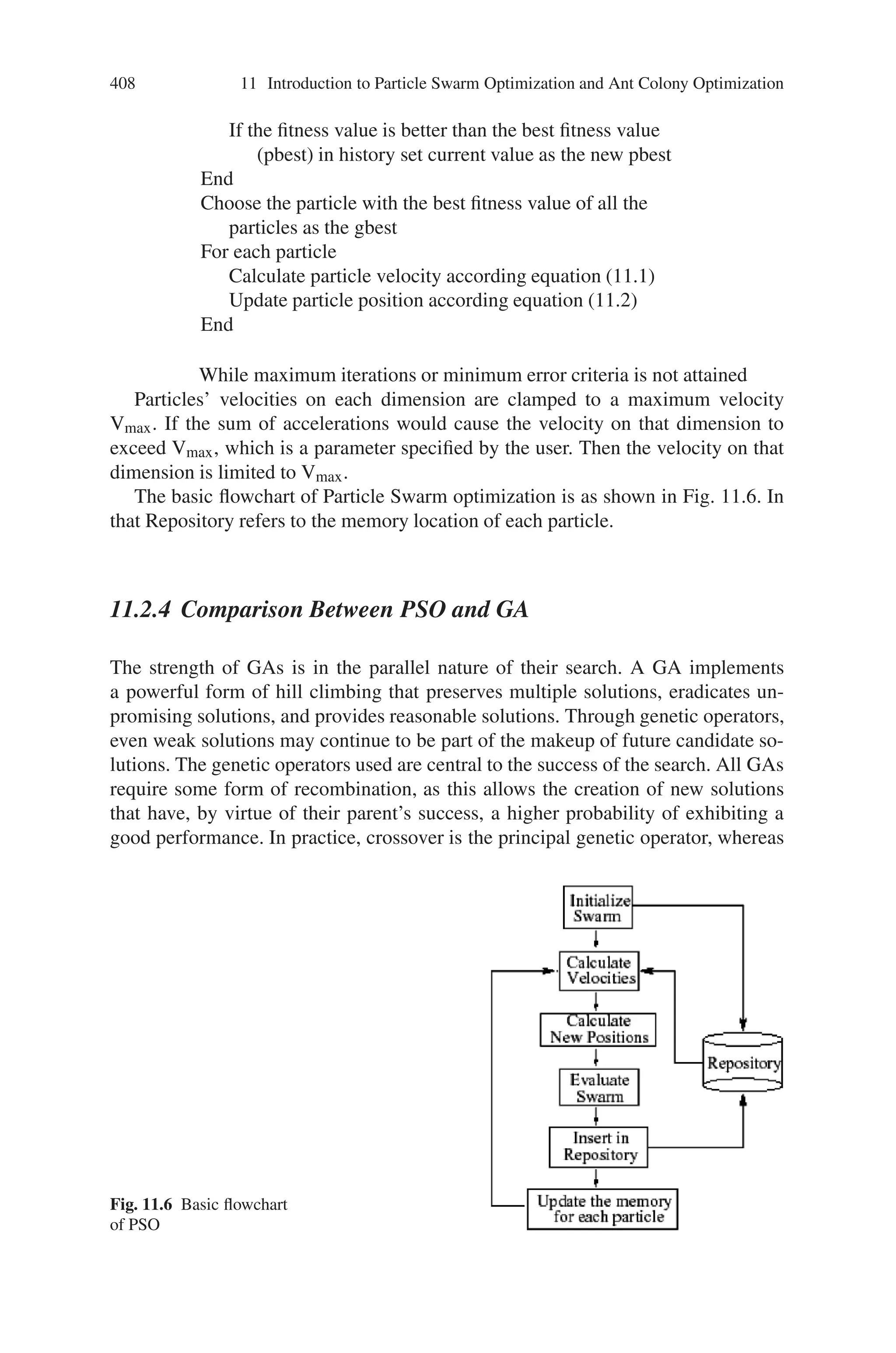
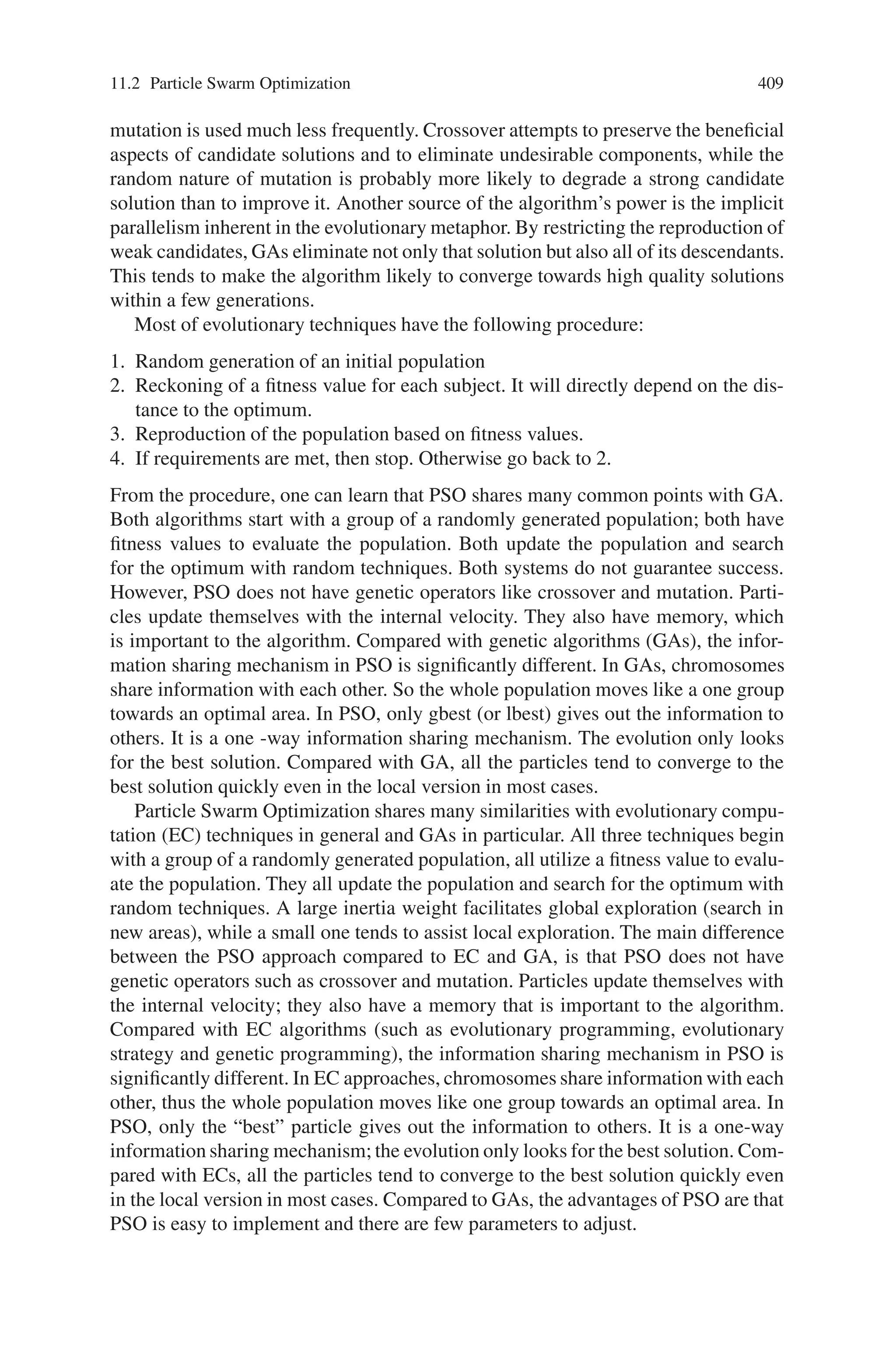
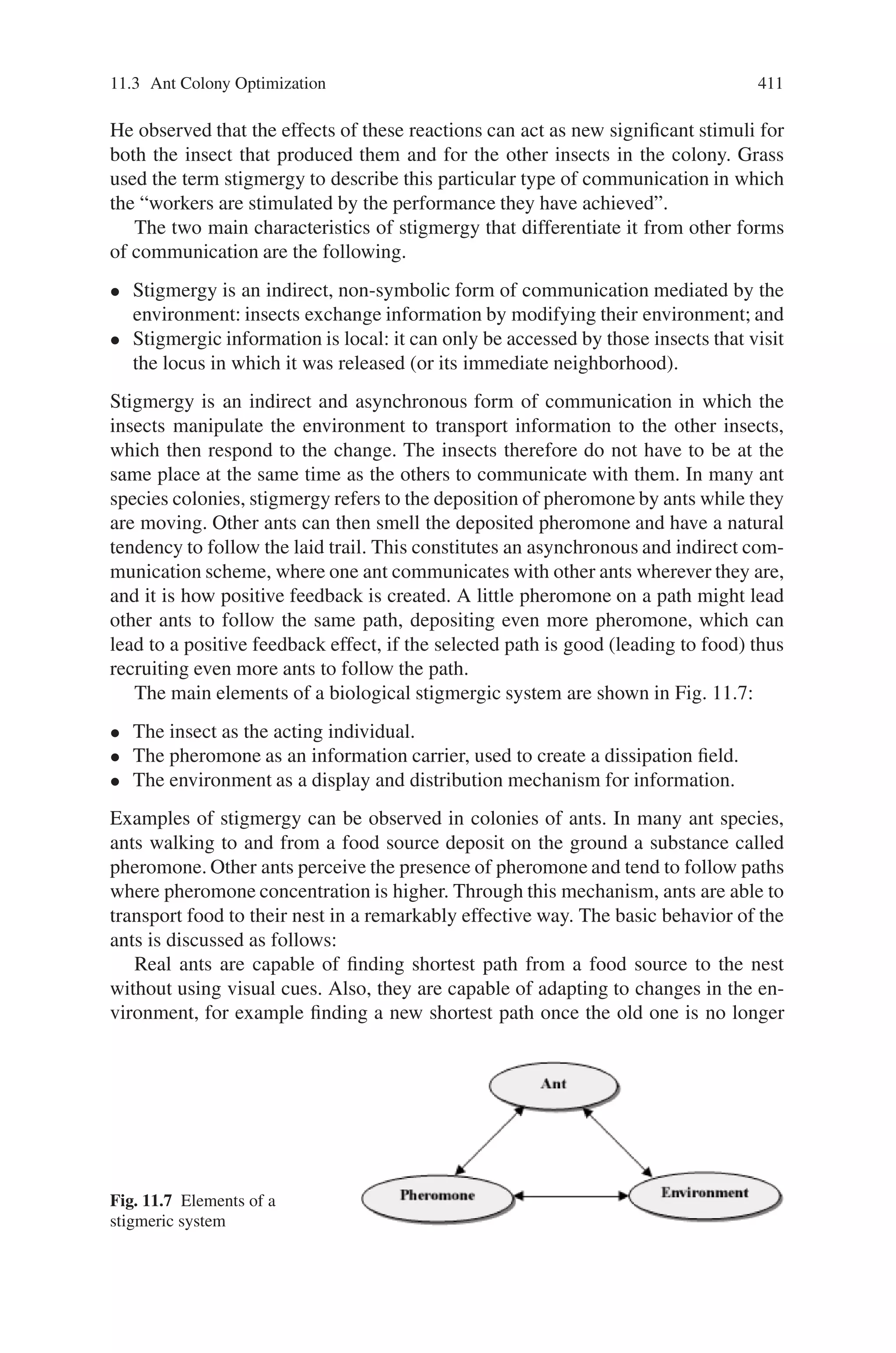
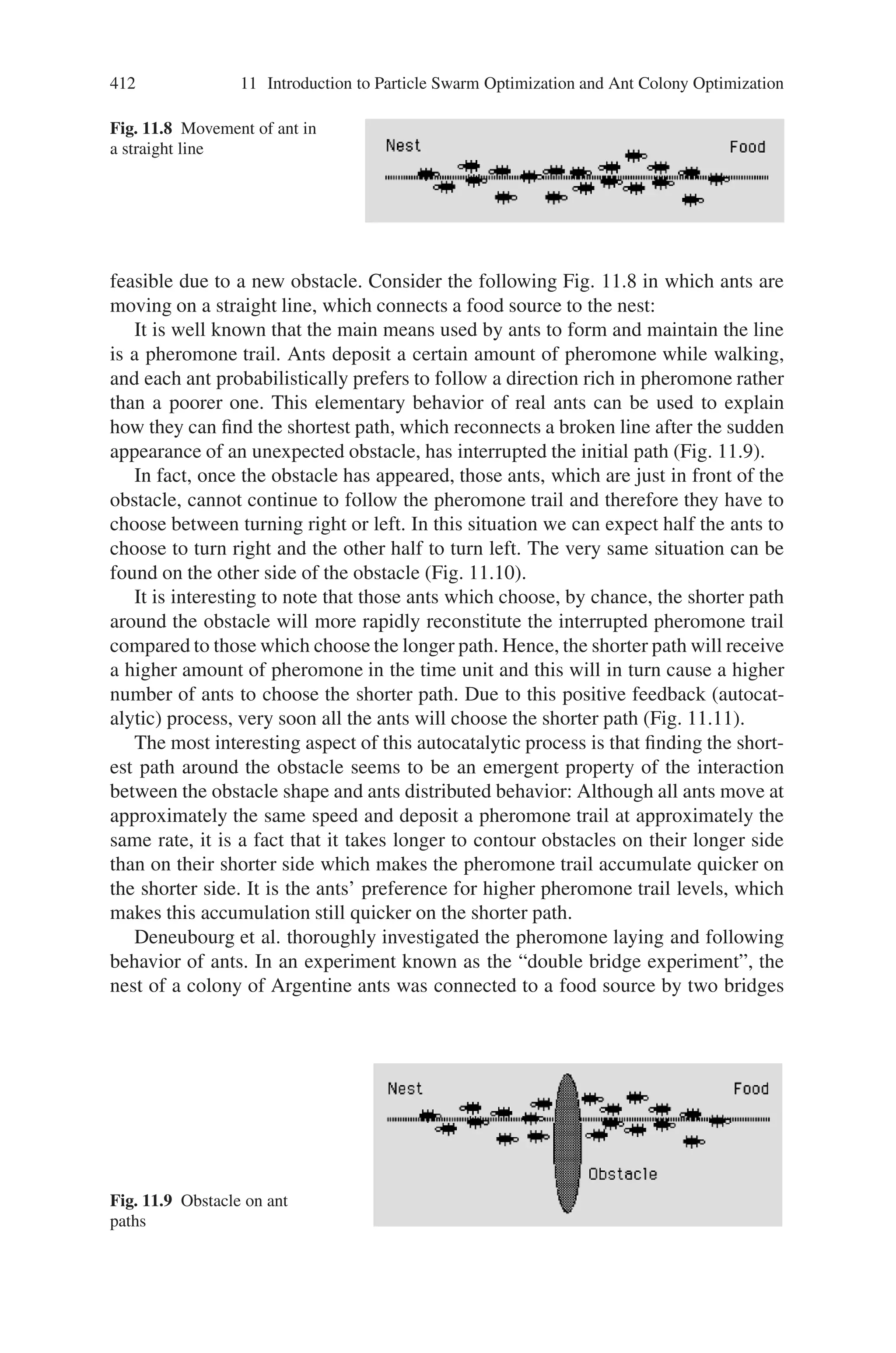
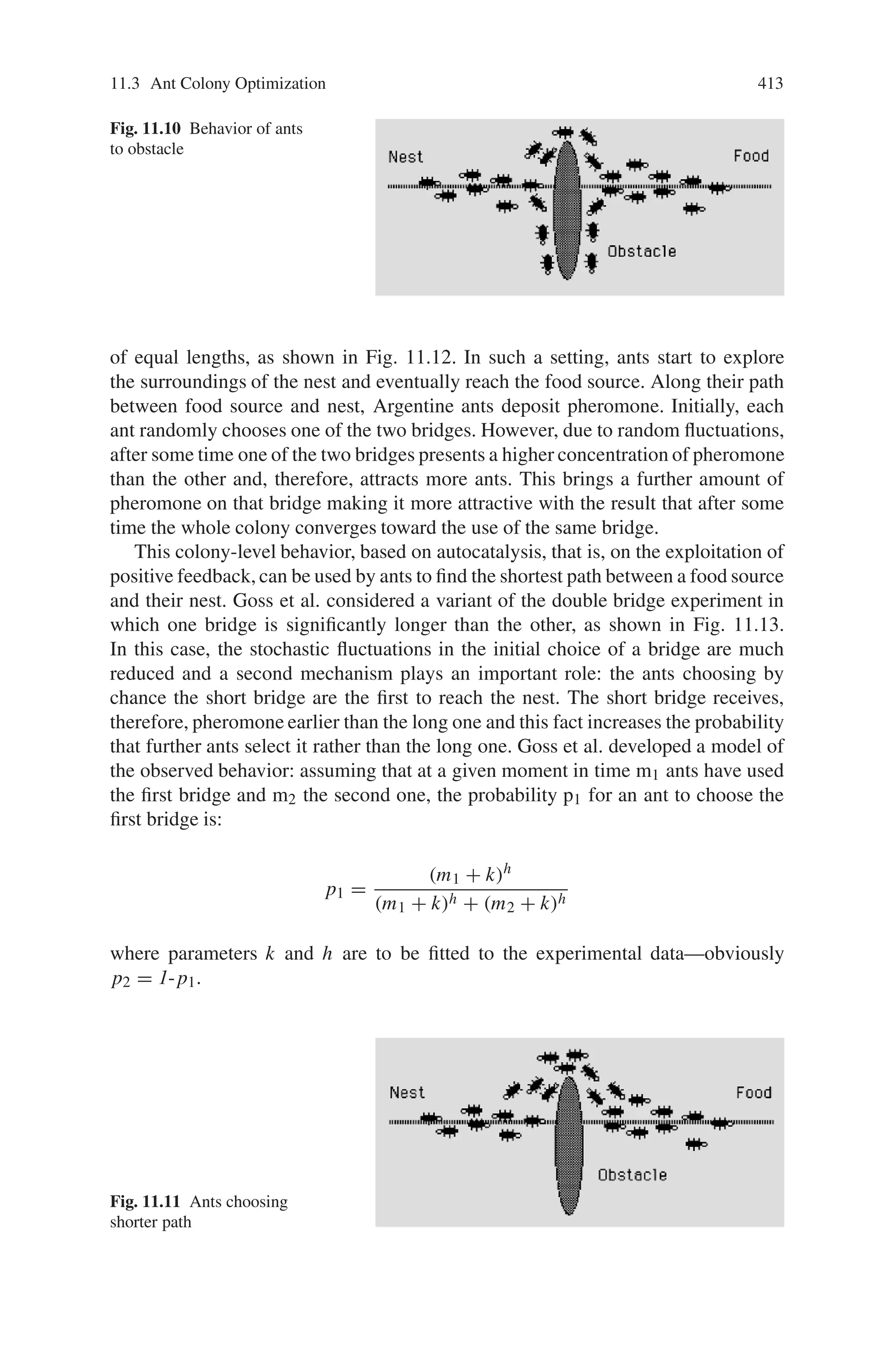
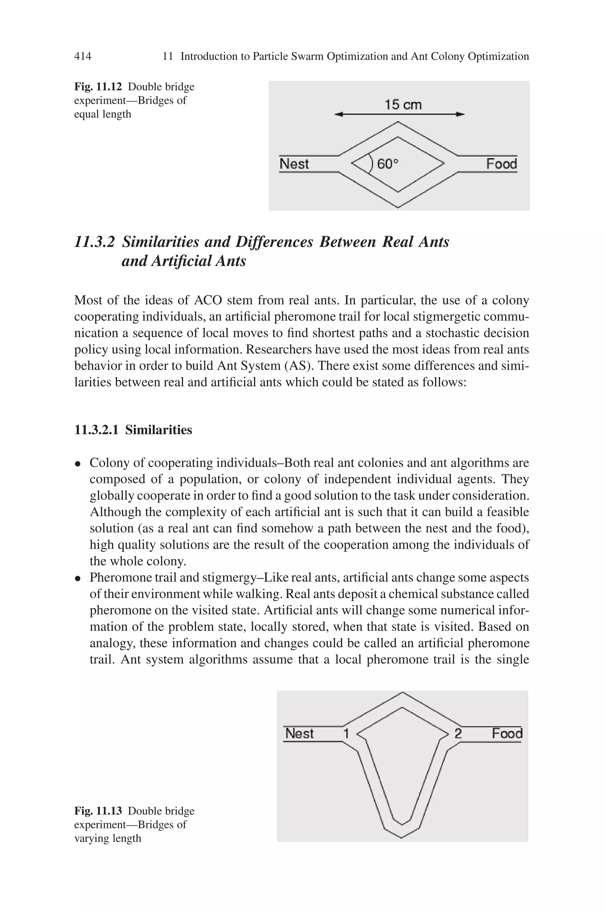

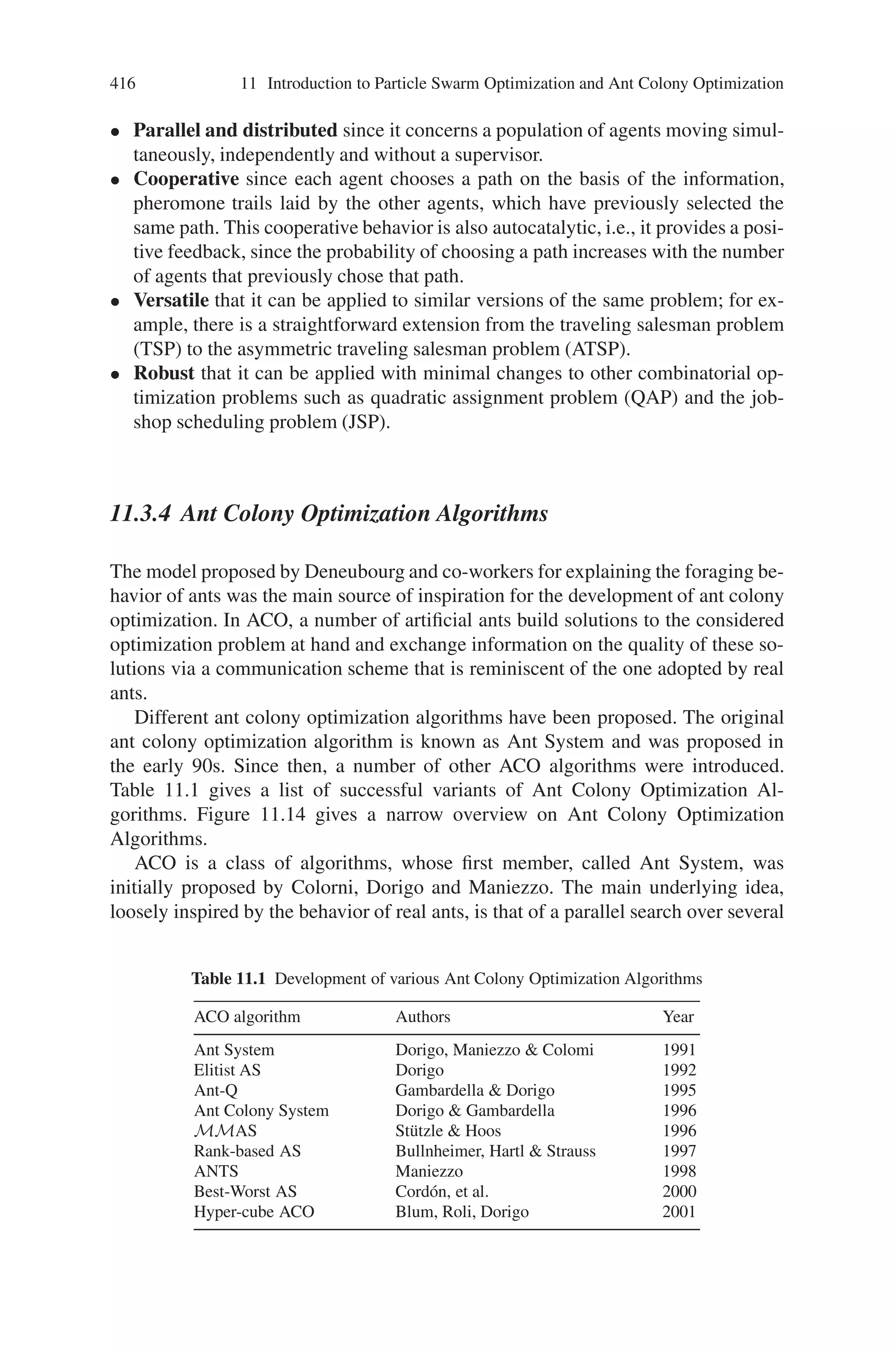
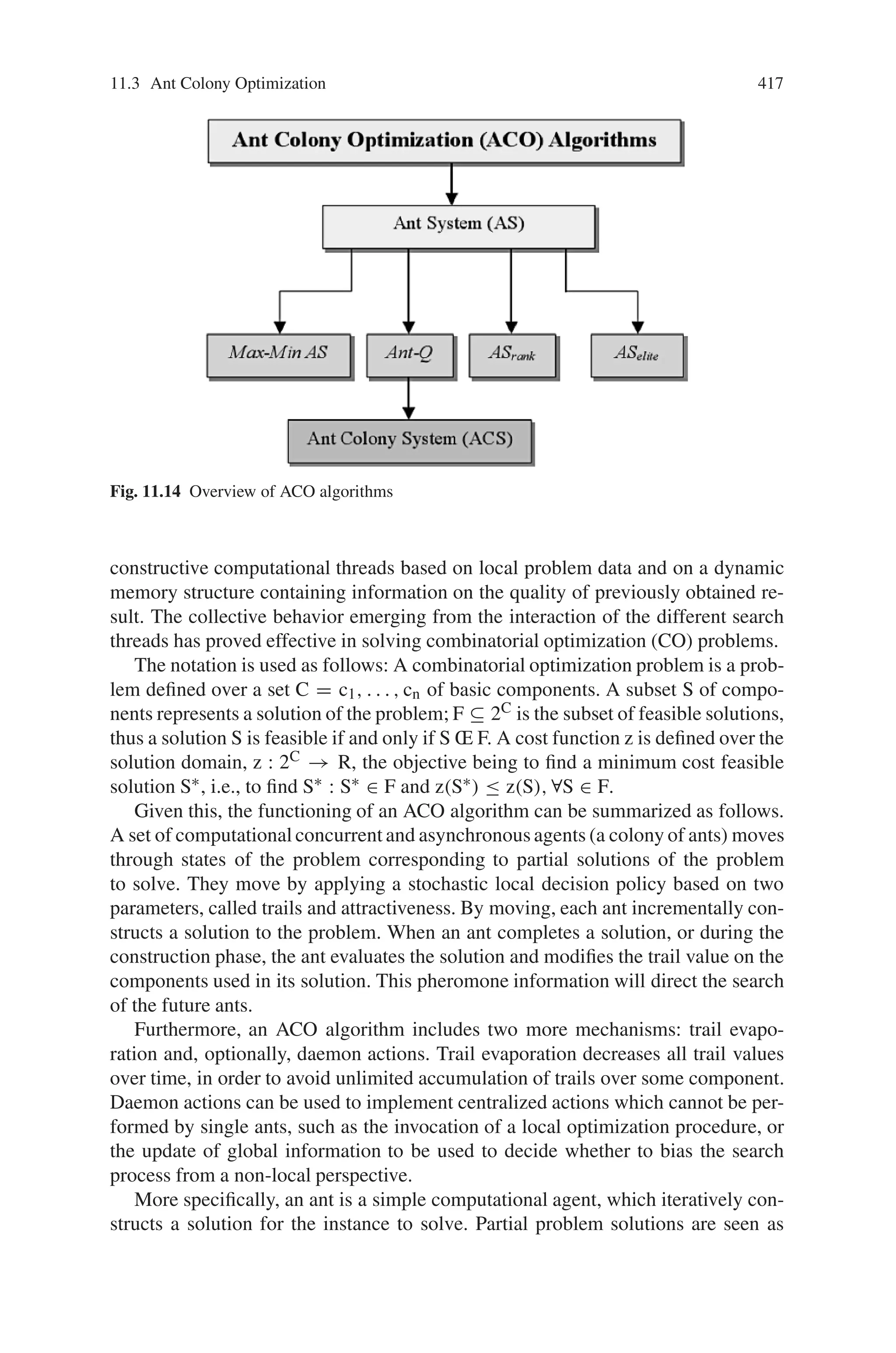
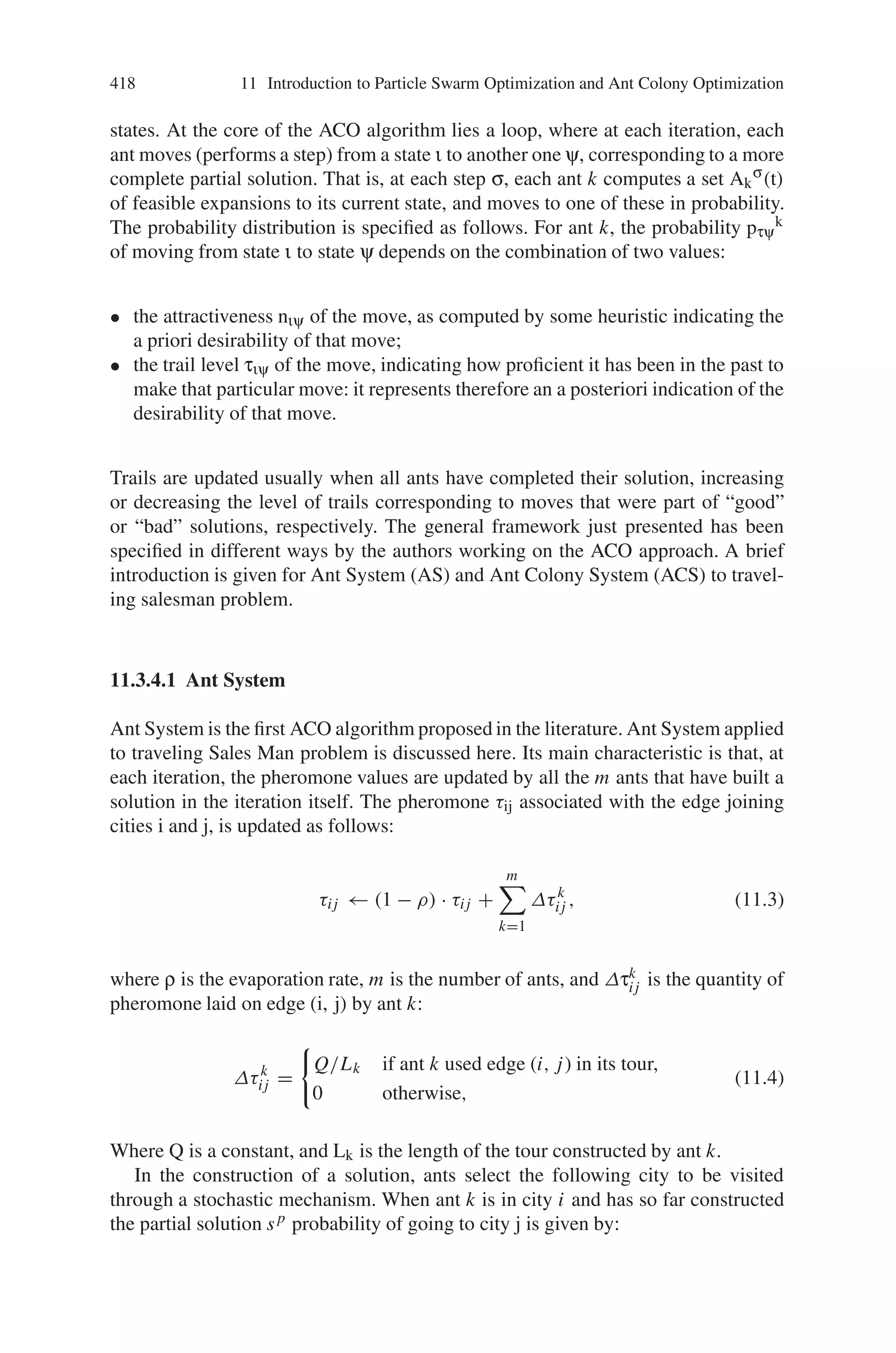
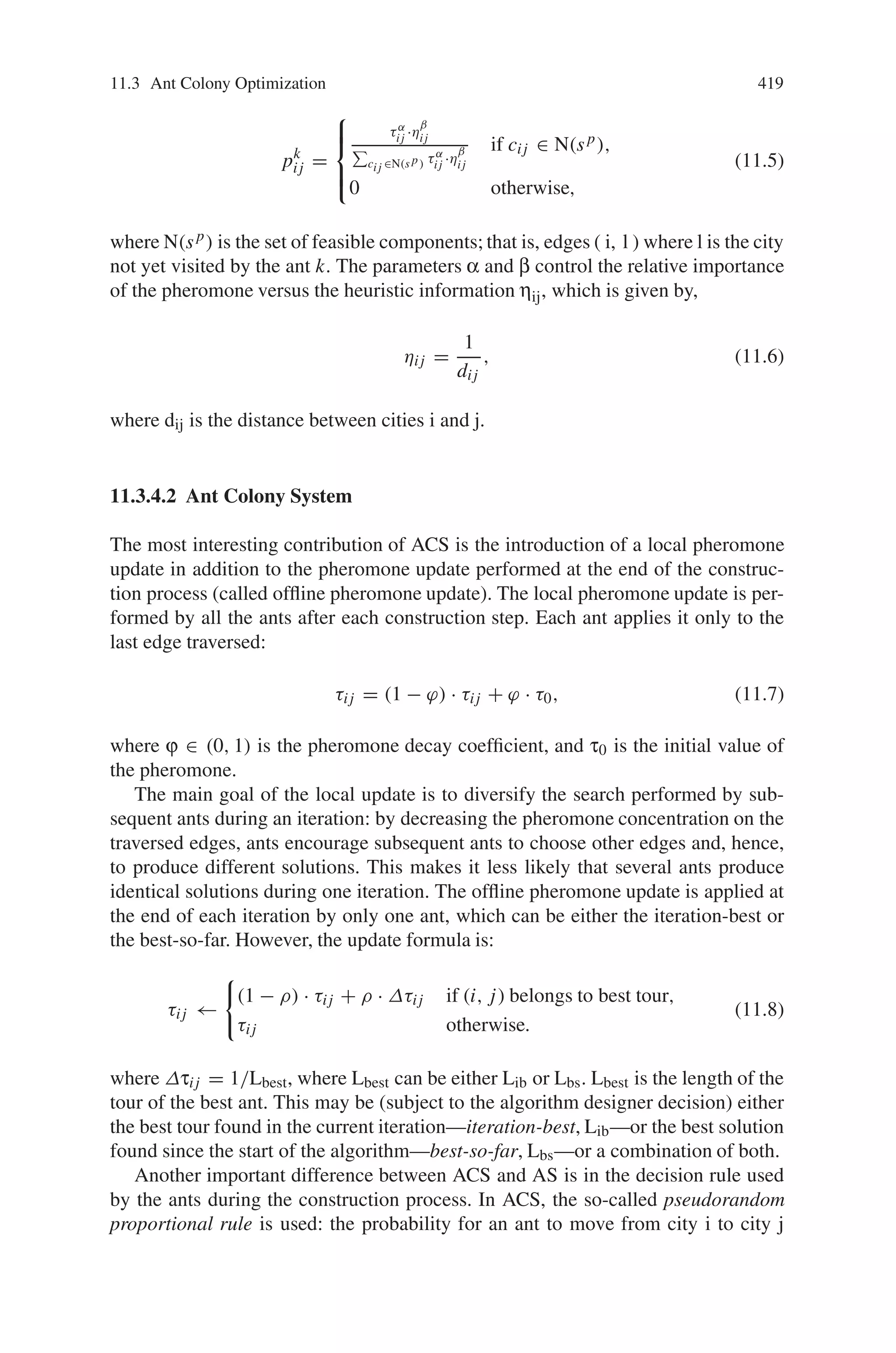
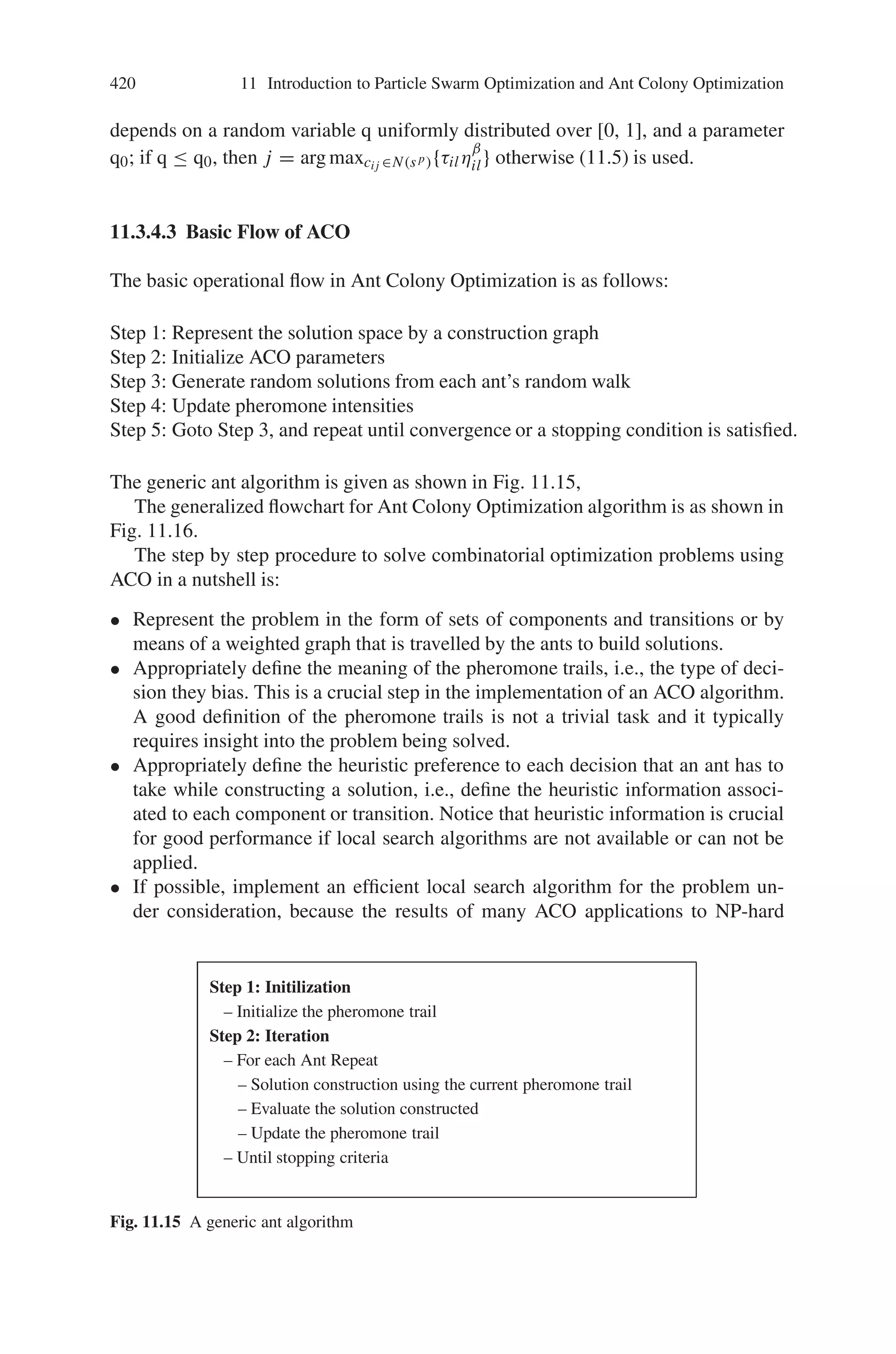
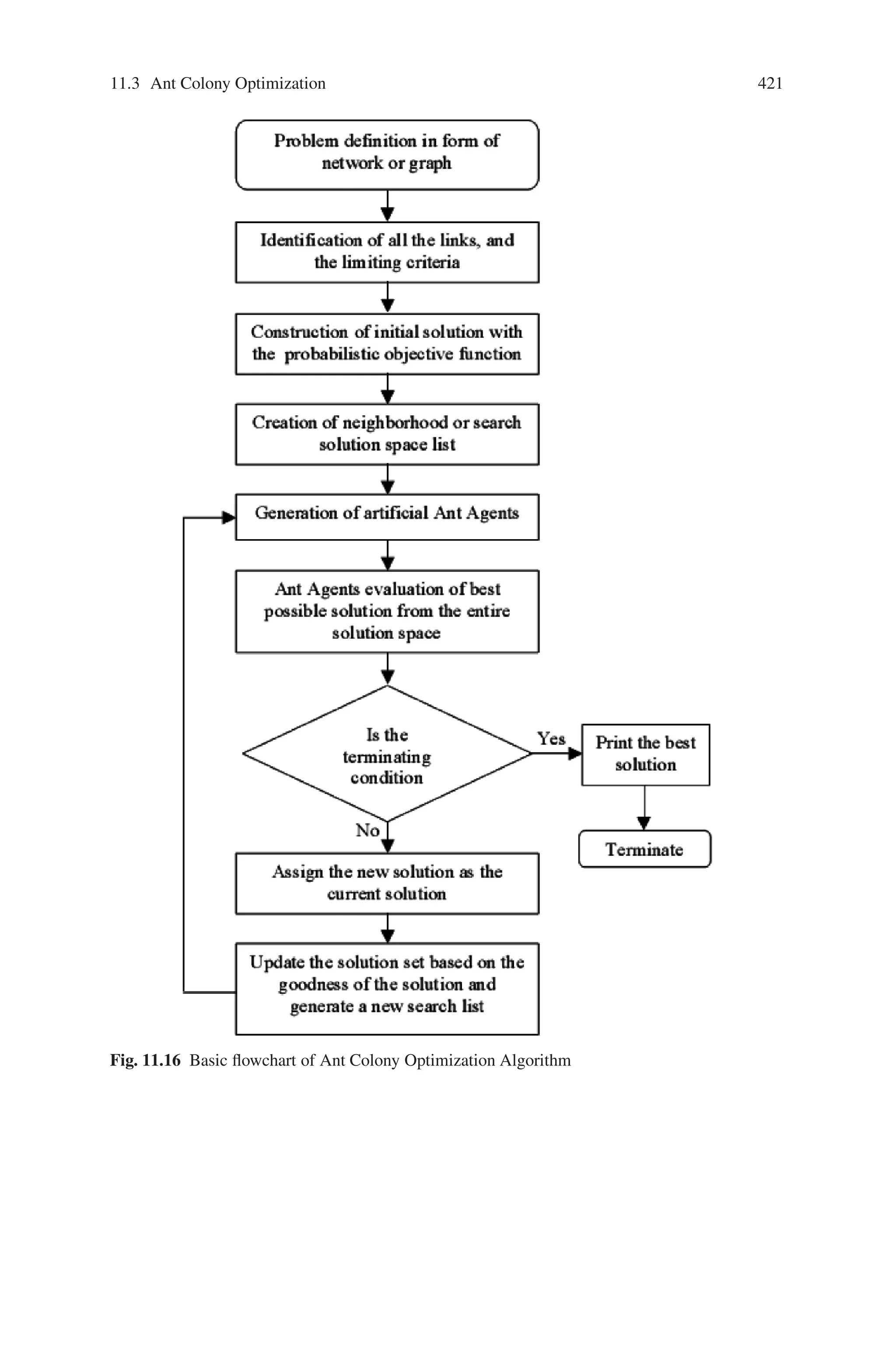
![420 11 Introduction to Particle Swarm Optimization and Ant Colony Optimization
depends on a random variable q uniformly distributed over [0, 1], and a parameter
q0; if q ≤ q0, then j = arg maxcij ∈N(s p){τilη
β
il} otherwise (11.5) is used.
11.3.4.3 Basic Flow of ACO
The basic operational flow in Ant Colony Optimization is as follows:
Step 1: Represent the solution space by a construction graph
Step 2: Initialize ACO parameters
Step 3: Generate random solutions from each ant’s random walk
Step 4: Update pheromone intensities
Step 5: Goto Step 3, and repeat until convergence or a stopping condition is satisfied.
The generic ant algorithm is given as shown in Fig. 11.15,
The generalized flowchart for Ant Colony Optimization algorithm is as shown in
Fig. 11.16.
The step by step procedure to solve combinatorial optimization problems using
ACO in a nutshell is:
• Represent the problem in the form of sets of components and transitions or by
means of a weighted graph that is travelled by the ants to build solutions.
• Appropriately define the meaning of the pheromone trails, i.e., the type of deci-
sion they bias. This is a crucial step in the implementation of an ACO algorithm.
A good definition of the pheromone trails is not a trivial task and it typically
requires insight into the problem being solved.
• Appropriately define the heuristic preference to each decision that an ant has to
take while constructing a solution, i.e., define the heuristic information associ-
ated to each component or transition. Notice that heuristic information is crucial
for good performance if local search algorithms are not available or can not be
applied.
• If possible, implement an efficient local search algorithm for the problem un-
der consideration, because the results of many ACO applications to NP-hard
Step 1: Initilization
– Initialize the pheromone trail
Step 2: Iteration
– For each Ant Repeat
– Solution construction using the current pheromone trail
– Evaluate the solution constructed
– Update the pheromone trail
– Until stopping criteria
Fig. 11.15 A generic ant algorithm](https://image.slidesharecdn.com/s-220425101513/75/S-N-Sivanandam-S-N-Deepa-Introduction-to-Genetic-Algorithms-2008-ISBN-3540731894-pdf-433-2048.jpg)