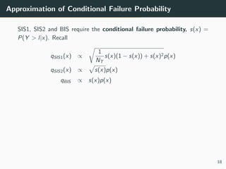
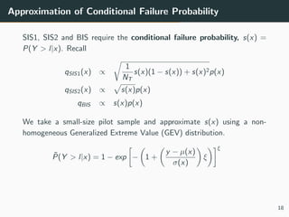
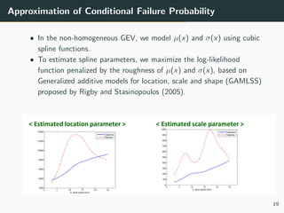
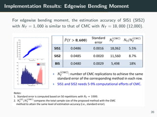
Download to read offline


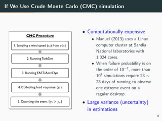
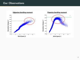
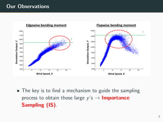
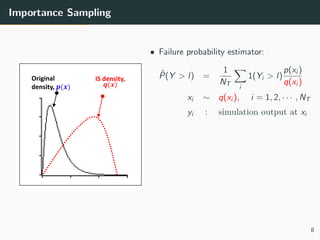


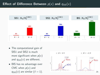
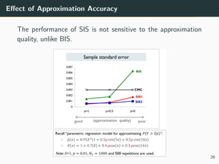
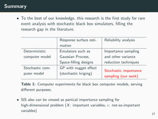

This document discusses the use of variance reduction techniques, specifically importance sampling, for reliability assessment in wind turbine design utilizing stochastic computer models. The research highlights the limitations of conventional Monte Carlo simulations and introduces a novel approach that optimally allocates computational resources to estimate failure probabilities more accurately and efficiently. Future plans include exploring new modeling techniques and extending the approach to address multiple outputs and high-dimensional inputs.