Recommended
PDF
PPTX
05 classification 1 decision tree and rule based classification
PDF
วิทยาการคำนวณ ม.5 - บทที่ 1 ข้อมูลมีคุณค่า
PDF
บทที่ 7 การสร้างเว็บไซต์อีคอมเมิร์ซ
PPTX
01 introduction to data mining
PPTX
PPTX
07 classification 3 neural network
PPTX
บทที่ 3 แรง และ กฎการเคลื่อนที่ของนิวตัน
PPT
PDF
PDF
PDF
โจทย์ปัญหาค่าเฉลี่ยเลขคณิต
PDF
2.1การวิเคราะห์และนำเสนอข้อมูลเชิงคุณภาพด้วยตารางความถี่
PDF
PDF
วิทยาการคำนวณ ม.5 - บทที่ 2 การเก็บรวบรวมและสำรวจข้อมูล
PDF
สื่อประกอบการสอน_เรื่อง_สิ่งมีชีวิตดัดแปรพันธุกรรม_(1)-07171442.pdf
PPTX
PDF
PDF
PDF
วิทยาการคำนวณ ม.5 - บทที่ 4 การทำข้อมูลให้เป็นภาพ และการสื่อสารด้วยข้อมูล
PDF
PDF
05 entity relationship model
PDF
PDF
PPT
การวิเคราะห์อัลกอริทึม(algorithm analysis)
PDF
ความสัมพันธ์ระหว่าง ความต่างศักย์ไฟฟ้า กระแสไฟฟ้า และ ความต้านทานไฟฟ้า
PDF
PDF
หน่วยที่ 1-เทคโนโลยีรอบตัว
PDF
ติวสรุป เนื้อหาสถิติธุรกิจ Final 1.64.pdf
PPT
More Related Content
PDF
PPTX
05 classification 1 decision tree and rule based classification
PDF
วิทยาการคำนวณ ม.5 - บทที่ 1 ข้อมูลมีคุณค่า
PDF
บทที่ 7 การสร้างเว็บไซต์อีคอมเมิร์ซ
PPTX
01 introduction to data mining
PPTX
PPTX
07 classification 3 neural network
PPTX
บทที่ 3 แรง และ กฎการเคลื่อนที่ของนิวตัน
What's hot
PPT
PDF
PDF
PDF
โจทย์ปัญหาค่าเฉลี่ยเลขคณิต
PDF
2.1การวิเคราะห์และนำเสนอข้อมูลเชิงคุณภาพด้วยตารางความถี่
PDF
PDF
วิทยาการคำนวณ ม.5 - บทที่ 2 การเก็บรวบรวมและสำรวจข้อมูล
PDF
สื่อประกอบการสอน_เรื่อง_สิ่งมีชีวิตดัดแปรพันธุกรรม_(1)-07171442.pdf
PPTX
PDF
PDF
PDF
วิทยาการคำนวณ ม.5 - บทที่ 4 การทำข้อมูลให้เป็นภาพ และการสื่อสารด้วยข้อมูล
PDF
PDF
05 entity relationship model
PDF
PDF
PPT
การวิเคราะห์อัลกอริทึม(algorithm analysis)
PDF
ความสัมพันธ์ระหว่าง ความต่างศักย์ไฟฟ้า กระแสไฟฟ้า และ ความต้านทานไฟฟ้า
PDF
PDF
หน่วยที่ 1-เทคโนโลยีรอบตัว
Similar to 06 classification 2 bayesian and instance based classification
PDF
ติวสรุป เนื้อหาสถิติธุรกิจ Final 1.64.pdf
PPT
PPT
การสร้างและหาคุณภาพศูนย์วิทย์(ดร.จันทิมา)
PPT
การสร้างและหาคุณภาพศูนย์วิทย์(ดร.จันทิมา)
PDF
Statistics for research by spss program
PPTX
03-Data-Exploration.en.th.pptx
PDF
PDF
PPT
PPT
PDF
PPT
PDF
สถิติเบื้องต้นกลุ่ม 2 สำรอง
PDF
สถิติเบื้องต้นกลุ่ม 2 สำรอง
PDF
%Ca%c3%d8%bb%ca%b6%d4%b5%d4%5 b1%5d
PPT
DOCX
DOC
PDF
12 งานนำสนอ cluster analysis
PPT
ความรู้เบื้องต้นเกี่ยวกับสถิติ อภิเทพ
More from นนทวัฒน์ บุญบา
PPTX
TXT
PPTX
PPT
PPTX
PPTX
PPTX
PPTX
06 classification 2 bayesian and instance based classification 1. 2. 3. 4. ทฤษฎีของเบย์ (Bayesian theorem)
ให้ D แทนข้อมูลที่นามาใช้ในการคานวณการแจกแจงความน่าจะเป็น
posteriori probability ของสมมติฐาน h คือ P(h|D) ตามทฤษฎี
P(h) คือ ความน่าจะเป็นก่อนหน้าของสมมติฐาน h
P(D) คือ ความน่าจะเป็นก่อนหน้าของชุดข้อมูลตัวอย่าง D
P(h|D) คือ ความน่าจะเป็นของ h เมื่อรู้ D
P(D|h) คือ ความน่าจะเป็นของ D เมื่อรู้ h
4
5. ตัวอย่าง:: การพยากรณ์อากาศ
การพยากรณ์อากาศ (Weatherforecast)
ความน่าจะเป็นที่เกิดเฮอร์ริเคนในชิคาโก้คือ 0.008
ทอมมีทักษะในการพยากรณ์ถูกต้องประมาณ 98% ของการทานายทั้งหมด (Predict-hur)
แต่ทอมก็มีการทานายถูกว่าไม่เกิดเฮอร์ริเคนถูกต้อง 97% เช่นกัน (Predict-nohur)
P(hurricane) = 0.008
P(~hurricane) = 1 – P(hurricane)
= 0.992
P(~h)
P(h)
P(~h) = 1- P(h)
P(h) + P(~h) = 1
5
6. ตัวอย่าง:: การพยากรณ์อากาศ
การพยากรณ์อากาศ (Weather forecast)
ความน่าจะเป็นที่เกิดเฮอร์ริเคนในชิคาโก้คือ 0.008
ทอมมีทักษะในการพยากรณ์ถูกต้องประมาณ 98% ของการทานายทั้งหมด (Predict-hur)
แต่ทอมก็มีการทานายถูกว่าไม่เกิดเฮอร์ริเคนถูกต้อง 97% เช่นกัน (Predict-nh)
P(hurricane) = 0.008
P(predict-hur | hurricane) = 0.98
P(predict-nohur | hurricane) = 0.02
P(~hurricane) = 0.992
P(hurricane)
P(predict-h)
= 0.98
P(predict-nh)= 0.02
6
7. ตัวอย่าง:: การพยากรณ์อากาศ
การพยากรณ์อากาศ (Weatherforecast)
ความน่าจะเป็นที่เกิดเฮอร์ริเคนในชิคาโก้คือ 0.008
ทอมมีทักษะในการพยากรณ์ถูกต้องประมาณ 98% ของการทานายทั้งหมด (Predict-hur)
แต่ทอมก็มีการทานายถูกว่าไม่เกิดเฮอร์ริเคนถูกต้อง 97%
(Predict-nohur)
P(hurricane) = 0.008
P(predict-h|hurricane) = 0.98
P(predict-nh|hurricane) = 0.02
P(~hurricane) = 0.992
P(predict-h|~hurricane) = 0.03
P(predict-nh| ~hurricane) = 0.97
P(~hurricane)
P(predict-h)
= 0.03
P(predict-nh) = 0.97
7
8. ตัวอย่าง:: การพยากรณ์อากาศ
ถ้าสุ่มวันขึ้นมา จากทักษะที่ทอมทานายการเกิดเฮอร์ริเคน จะเชื่อเขาหรือไม่??
ความน่าจะเป็นที่เขาทานายถูกต้อง?
ความน่าจะเป็นที่เขาทานายผิด?
P(p-h|h)P(h)
P(p-h)
P(h|p-h) = 0.98*0.008 0.0078==
P(hurricane) = 0.008
P(predict-h|hurricane) = 0.98
P(predict-nh|hurricane) = 0.02
P(~hurricane) = 0.992
P(predict-h|~hurricane) = 0.03
P(predict-nh| ~hurricane) = 0.97
P(p-h|~h)P(~h)
P(p-h)
P(~h|p-h) = 0.03*0.992 0.0298= =
8
9. ตัวอย่าง:: มะเร็ง (Cancer)
คนไข้คนหนึ่งไปตรวจหามะเร็ง ผลการตรวจเป็นบวก(+) อยากทราบว่า เราควร
วินิจฉัยโรคคนไขคนนี้ว่าเป็นมะเร็งจริงหรือไม่? ความเป็นจริง คือ
ผลการตรวจเมื่อเป็นบวกจะให้ความถูกต้อง98% กรณีที่มีโรคนั้นอยู่จริง
ผลการตรวจเมื่อเป็นลบจะให้ความถูกต้อง 97% กรณีที่ไม่มีโรคนั้น
0.008 ของประชากรทั้งหมดเป็นโรคมะเร็ง
จากความน่าจะเป็นข้างต้น เราจะทราบว่าความน่าจะเป็นต่อไปนี้
P(cancer)= P(~cancer) =
P(+ | cancer) = P(- | cancer) =
P(+ |~ cancer) = P(- |~ cancer) =
9
10. ตัวอย่าง:: มะเร็ง (Cancer)
เราสามารถคานวณค่าความน่าจะเป็นของสมมติฐานว่าคนไข้เป็น / ไม่เป็น
โรคมะเร็ง เมื่อทราบผลตรวจเป็นบวก โดยใช้กฎของเบย์ ดังนี้
ความน่าจะเป็นที่คนไข้คนนี้จะเป็นโรคมะเร็งเมื่อผลตรวจเป็นบวก เท่ากับ
P(cancer |+) =
ความน่าจะเป็นที่คนไข้คนนี้จะไม่เป็นโรคมะเร็งเมื่อผลตรวจเป็นบวก เท่ากับ
P(~cancer |+) =
P(+|cancer)P(cancer) =
P(+|~cancer)P(~cancer) =
10
11. วิธีการเรียนรู้เบย์อย่างง่าย (Naïve Bayesian Learning)
วิธีการของ Naïve Bayesian คือการใช้วิธีการของเบย์พร้อมสมมติฐานของการ
เป็นอิสระต่อกันของตัวแปรอิสระทุกตัว
โดยแต่ละ instance x มี n แอททริบิวต์ หรือ x= {A1, …, An} และมี Ci เป็น
class label
Naïve Bayes Classifier = Max (P(Ci) P(Aj |Ci) )
P(A1,…, An)
C = Max P’(Ci) P’(Aj |Ci)
n
i=1
m
j=1
11
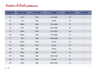
12. ตัวอย่าง: ผิวไหม้ (subburn)
Sample ID Hair color Eye Color Weight Apply lotion Sun burn
S1 black Dark overweight No -
S2 red Dark normal No +
S3 Blonde light Overweight No +
S4 Red light underweight No +
S5 Black Dark Overweight Yes -
S6 Blonde Dark Overweight No +
S7 Red light underweight Yes -
S8 Black Dark Normal No -
S9 Blonde Dark Normal Yes +
S10 Red light Normal Yes +
S11 Black light Normal Yes +
S12 Blonde light Underweight No +
S13 Red Dark Normal Yes -
S14 black light underweight no +
12
13. ตัวอย่าง: ผิวไหม้ (subburn)
Instance x = <hair color=red, eye color = dark, weight= overweight, apply lotion = no>
เพราะฉะนั้น เมื่อ instance ใหม่เข้ามาถามว่าผิวจะไหม้หรือไม่
C1 : sun burn is + :
P(+).P(red|+).P(dark|+).P(overweight|+).P(applylotion|+)
C2 : sun burn is - :
P(-).P(red|-).P(dark|-).P(overweight|-).P(applylotion|-)
01.0
9
6
9
2
9
3
9
3
14
9
018.0
5
2
5
2
5
4
5
2
14
5
X belongs to class (“sunburn = -”)
13
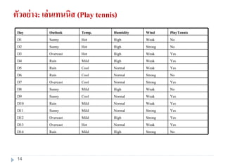
14. ตัวอย่าง: เล่นเทนนิส (Play tennis)
NoStrongHighMildRainD14
YesWeakNormalHotOvercastD13
YesStrongHighMildOvercastD12
YesStrongNormalMildSunnyD11
YesWeakNormalMildRainD10
YesWeakNormalCoolSunnyD9
NoWeakHighMildSunnyD8
YesStrongNormalCoolOvercastD7
NoStrongNormalCoolRainD6
YesWeakNormalCoolRainD5
YesWeakHighMildRainD4
YesWeakHighHotOvercastD3
NoStrongHighHotSunnyD2
NoWeakHighHotSunnyD1
PlayTennisWindHumidityTemp.OutlookDay
14
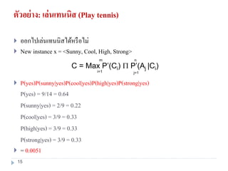
15. ตัวอย่าง: เล่นเทนนิส (Play tennis)
ออกไปเล่นเทนนิสได้หรือไม่
New instance x = <Sunny, Cool, High, Strong>
P(yes)P(sunny|yes)P(cool|yes)P(high|yes)P(strong|yes)
P(yes) = 9/14 = 0.64
P(sunny|yes) = 2/9 = 0.22
P(cool|yes) = 3/9 = 0.33
P(high|yes) = 3/9 = 0.33
P(strong|yes) = 3/9 = 0.33
= 0.0051
C = Max P’(Ci) P’(Aj |Ci)
n
i=1
m
j=1
15
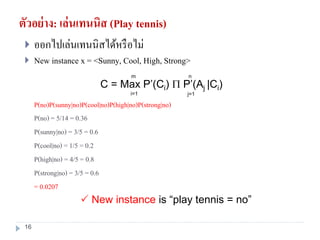
16. ตัวอย่าง: เล่นเทนนิส (Play tennis)
ออกไปเล่นเทนนิสได้หรือไม่
New instance x = <Sunny, Cool, High, Strong>
P(no)P(sunny|no)P(cool|no)P(high|no)P(strong|no)
P(no) = 5/14 = 0.36
P(sunny|no) = 3/5 = 0.6
P(cool|no) = 1/5 = 0.2
P(high|no) = 4/5 = 0.8
P(strong|no) = 3/5 = 0.6
= 0.0207
C = Max P’(Ci) P’(Aj |Ci)
n
i=1
m
j=1
New instance is “play tennis = no”
16
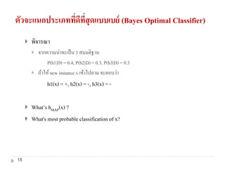
17. 18. ตัวจะแนกประเภทที่ดีที่สุดแบบเบย์ (Bayes Optimal Classifier)
พิจารณา
จากความน่าจะเป็น 3 สมมติฐาน
P(h1|D) = 0.4, P(h2|D) = 0.3, P(h3|D) = 0.3
ถ้าให้new instance x เข้าไปถาม จะตอบว่า
h1(x) = +, h2(x) = -, h3(x) = -
What’s hMAP(x) ?
What's most probable classification of x?
18
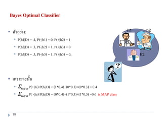
19. Bayes Optimal Classifier
ตัวอย่าง:
P(h1|D) = .4, P(-|h1) = 0, P(+|h2) = 1
P(h2|D) = .3, P(-|h2) = 1, P(+|h3) = 0
P(h3|D) = .3, P(-|h3) = 1, P(+|h3) = 0,
เพราะฉะนั้น
hi H P(+|hi) P(hi|D) = (1*0.4)+(0*0.3)+(0*0.3) = 0.4
hi H P( -|hi) P(hi|D) = (0*0.4)+(1*0.3)+(1*0.3) =0.6 is MAP class
h1 h2
h3
19
20. 21. Lazy & Eager Learning
Lazy learning (e.g., Instance-based learning): เป็นการเรียนรู้อย่างง่ายโดยใช้การ
สารวจชุดข้อมูลสอนคร่าวๆ และรอจนกระทั่งถึงเวลาทดสอบจึงจาแนกประเภท
ข้อมูล
Eager learning (e.g. Decision trees): ใช้เวลาในการเรียนรู้จากชุดข้อมูลสอนก่อนเป็น
เวลานาน แต่หลังจากที่ทาการเรียนรู้เรียบร้อยแล้ว สามารถนาชุดทดสอบจาแนก
ประเภทได้เวลาอันรวดเร็ว
Its very similar to a
Desktop!!
Eager
Survey before
21
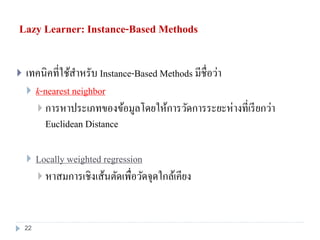
22. Lazy Learner: Instance-Based Methods
เทคนิคที่ใช้สาหรับ Instance-Based Methods มีชื่อว่า
k-nearest neighbor
การหาประเภทของข้อมูลโดยให้การวัดการระยะห่างที่เรียกว่า
Euclidean Distance
Locally weighted regression
หาสมการเชิงเส้นตัดเพื่อวัดจุดใกล้เคียง
22
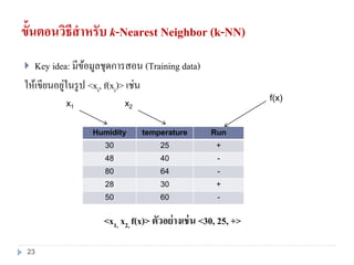
23. ขั้นตอนวิธีสาหรับ k-Nearest Neighbor (k-NN)
Key idea: มีข้อมูลชุดการสอน (Training data)
ให้เขียนอยู่ในรูป <xi, f(xi)> เช่น
Humidity temperature Run
30 25 +
48 40 -
80 64 -
28 30 +
50 60 -
x1 x2
f(x)
<x1, x2, f(x)> ตัวอย่างเช่น <30, 25, +>
23
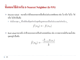
24. ขั้นตอนวิธีสาหรับ k-Nearest Neighbor (k-NN)
Discrete-valued หมายถึง ค่าป้ ายบอกฉลากเป็นที่แบ่งประเภทชัดเจน เช่น วิ่ง หรือ ไม่วิ่ง ใช่
หรือ ไม่ใช่ เป็นต้น
ดังนั้นหาชุด xq, ที่ใกล้เคียงที่สุดสาหรับชุดข้อมูลสอนมาเป็นตัวประมาณค่าสาหรับ xn
Real-valued หมายถึง ค่าป้ ายบอกฉลากเป็นตัวเลขทศนิยม เช่น การพยากรณ์ปริมาณน้าฝน
อุณหภูมิ เป็นต้น
24
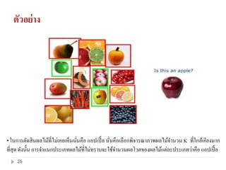
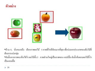
25. 26. ตัวอย่าง
•ถ้า k=5, นั่นหมายถึง เลือกภาพผลไม้ 5 ภาพที่ใกล้เคียงมากที่สุด เพื่อบ่งบอกประเภทของต้นไม้ที่
ต้องการแบ่งกลุ่ม
•ดังนั้นจากภาพจะเห็นได้ว่า ผลไม้ทั้ง 5 ภาพส่วนใหญ่เป็นภาพของ แอปเปิ้ล ดังนั้นจึงตอบผลไม้นี้ว่า
เป็นแอบเปิ้ล
26
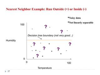
27. Nearest Neighbor Example: Run Outside (+) or Inside (-)
Humidity
Temperature
0
100
0 100
+
+
+
+
-
-
-
-
-
-
-
+
+
•Noisy data
•Not linearly separable
Decision tree boundary (not very good...)
?
?
?
?
-
-
?
?
?
27
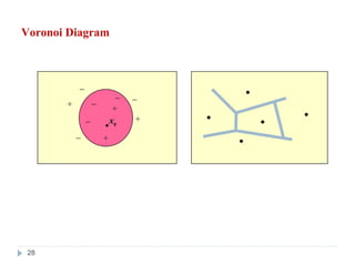
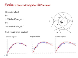
28. 29. ตัวอย่าง: K-Nearest Neighbor กับ Voronoi
(Discrete-valued)
k=1
1-NN classifies xq as +
k=5
5-NN classifies xq as −
(real-valued target function)
29
30. เมื่อไหร่ถึงจะใช้ k-Nearest Neighbor
เมื่อชุดข้อมูลสามารถแปลงให้อยู่ระนาบของมิติได้ ℜn
มี Attribute น้อยว่า 20 ตัว
มีข้อมูลชุดการสอน (Training data) เป็นจานวนมาก
ข้อดี
สอน (training) เร็วมาก
สามารถเรียนรู้กับฟังก์ชันที่ซับซ้อนได้
ไม่สูญเสียข้อมูลอื่น
ข้อเสีย
ช้าเวลาจาแนกประเภทข้อมูล
จะโง่เมื่อมีการคิด attribute ที่ไม่เกี่ยวข้อง
30
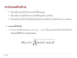
31. การกาหนดตัวแปร K
ไม่ควรเลือก K เล็กเกินไป เพราะจะทาให้เบี่ยงเบนสูง
ไม่ควรเลือก K ใหญ่เกินไป เพราะจะทาให้ข้อมูลเกินความลาเอียง
เพราะฉะนั้นการเลือกค่า K ขึ้นอยู่กับข้อมูล ต้องมีการปรับค่าการประเมินเช่น Cross-validation
ระยะทางที่ใช้วัด คือ
ถ้า x ประกอบไปด้วย Attribute <a1(x), a2(x), …, an(x)> ดังนั้น ar(x) ดังกล่าวจึงแทนด้วยค่าในด้วย x
ค่าระยะทางที่ใช้เรียกว่า Euclidean Distance
n
r
jrirji xaxaxxd
1
2
))()((),(
31
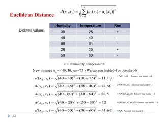
32. Euclidean Distance
Humidity temperature Run
30 25 +
48 40 -
80 64 -
28 30 +
50 60 -
x = <humidity, temperature>
New instance xq = <40, 30, run=?? > We can run inside(+)or outside (-)
n
r
jrirji xaxaxxd
1
2
))()((),(
18.11)2530()3040(),( 22
1 xxd q
80.12)4030()4840(),( 22
2 xxd q
5.52)6430()8040(),( 22
3 xxd q
1-NN (x1) Answer run inside (+)
2-NN (x1,x4) Answer run inside (+)
3-NN (x1,x2,x4)Answer run inside (+)
4-NN (x1,x2,x4,x5)Answer run inside (+)
5-NN Answer run inside (-)
12)3030()2840(),( 22
4 xxd q
62.31)6030()5040(),( 22
5 xxd q
Discrete values
32
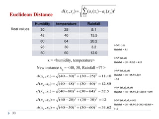
33. Euclidean Distance
Humidity temperature Rainfall
30 25 5.1
48 40 15.5
80 64 20.2
28 30 3.2
50 60 12.0
x = <humidity, temperature>
New instance xq = <40, 30, Rainfall =?? >
n
r
jrirji xaxaxxd
1
2
))()((),(
18.11)2530()3040(),( 22
1 xxd q
80.12)4030()4840(),( 22
2 xxd q
5.52)6430()8040(),( 22
3 xxd q
1-NN (x1)
Rainfall = 5.1
2-NN (x1,x4)
Rainfall = (5.1+3.2)/2 = 4.15
3-NN (x1,x2,x4)
Rainfall = (5.1+15.5+3.2)/3
= 7.9
4-NN (x1,x2,x4,x5)
Rainfall = (5.1+15.5+3.2+12.0)/4= 8.95
5-NN (x1,x2,x3, x4,x5)
Rainfall = (5.1+15.5+3.2+20.2+12.0)/5=
11.2
12)3030()2840(),( 22
4 xxd q
62.31)6030()5040(),( 22
5 xxd q
Real values
33
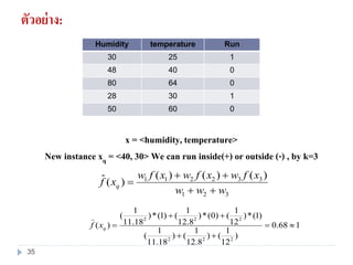
34. 35. ตัวอย่าง:
Humidity temperature Run
30 25 1
48 40 0
80 64 0
28 30 1
50 60 0
x = <humidity, temperature>
New instance xq = <40, 30> We can run inside(+) or outside (-) , by k=3
1 1 2 2 3 3
1 2 3
( ) ( ) ( )ˆ( )q
w f x w f x w f x
f x
w w w
168.0
)
12
1
()
8.12
1
()
18.11
1
(
)1(*)
12
1
()0(*)
8.12
1
()1(*)
18.11
1
(
)(
222
222
qxf
35
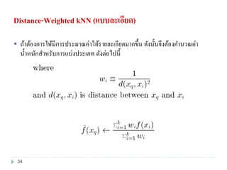
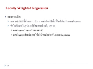
36. Locally Weighted Regression
แนวความคิด:
มาจาก k-NN ที่ค้นหาการประมาณค่าโดยใช้พื้นที่ใกล้เคียงในการประมาณ
ทาไมต้องอยู่ในรูปการใช้สมการเชิงเส้น เพราะ
ลดค่า error ในการกาหนดค่า K
ลดค่า error สาหรับการให้ค่าน้าหนักสาหรับการหา distance
36
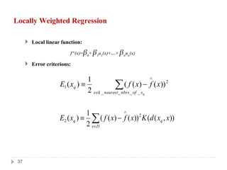
37. Locally Weighted Regression
Local linear function:
f^(x)=β0+ β1a1(x)+…+βnan(x)
Error criterions:
qxofnbrsnearestkx
q xfxfxE
____
2
1 ))()((
2
1
)(
)),(())()((
2
1
)( 2
2 xxdKxfxfxE q
Dx
q
37
38. Locally Weighted Regression
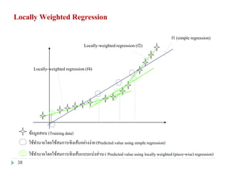
f1 (simple regression)
ข้อมูลสอน (Trainingdata)
ใช้ทานายโดยใช้สมการเชิงเส้นแบบแบ่งส่วน( Predictedvalue using locally weighted (piece-wise)regression)
ใช้ทานายโดยใช้สมการเชิงเส้นอย่างง่าย(Predictedvalue using simple regression)
Locally-weighted regression (f2)
Locally-weighted regression (f4)
38
39. HW#6
39
What is Bayesian Classification?
What is Naïve Bayesian Learning?
What is Instance-Based Classification?
Please explain Lazy & Eager Learning?
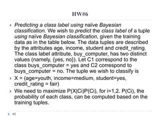
40. HW#6
40
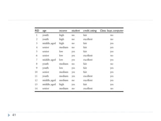
Predicting a class label using naïve Bayesian
classification. We wish to predict the class label of a tuple
using naïve Bayesian classification, given the training
data as in the table below. The data tuples are described
by the attributes age, income, student and credit_rating.
The class label attribute, buy_computer, has two distinct
values (namely, {yes, no}). Let C1 correspond to the
class buys_computer = yes and C2 correspond to
buys_computer = no. The tuple we wish to classify is
X = (age=youth, income=medium, student=yes,
credit_rating = fair)
We need to maximize P(X|Ci)P(Ci), for i=1,2. P(Ci), the
probability of each class, can be computed based on the
training tuples.
41. 42. LAB 6
42
Use weka program to construct a baysian network
classification and instance base classification from
the given file.
Labor.arff