MATLAB Sample
Scripts
With Electrical Engineering
Applications
Shameer A Koya
Introduction
 This lecture we will do some practice on Basic
MATLAB Scripts.
 We will start with simple scripts and will discuss
some electrical engineering applications.
 More scripts including conditional statements will
be discussed in the next lecture.
 Please review lectures on basic input and output
commands.
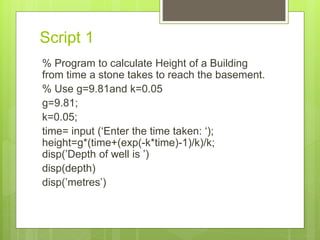
Script 1
% Program to calculate Height of a Building
from time a stone takes to reach the basement.
% Use g=9.81and k=0.05
g=9.81;
k=0.05;
time= input (‘Enter the time taken: ‘);
height=g*(time+(exp(-k*time)-1)/k)/k;
disp(’Depth of well is ’)
disp(depth)
disp(’metres’)
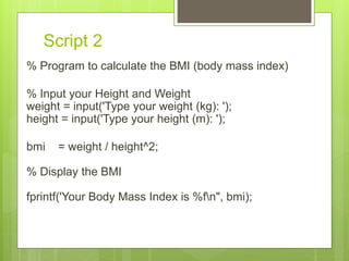
Script 2
% Program to calculate the BMI (body mass index)
% Input your Height and Weight
weight = input('Type your weight (kg): ');
height = input('Type your height (m): ');
bmi = weight / height^2;
% Display the BMI
fprintf('Your Body Mass Index is %fn", bmi);
Script 3
% Program to calculate Electricity bill.
w = input('Enter power of your device (in watts):
');
h = input('Enter time (in hours): ');
r = input('Enter electricity rate (in dollars per
KWH): ');
ec = w * h/1000 * r;
disp(’Your Electricity bill is’)
Disp(ec)
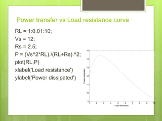
Power transfer vs Load resistance curve
RL = 1:0.01:10;
Vs = 12;
Rs = 2.5;
P = (Vs^2*RL)./(RL+Rs).^2;
plot(RL,P)
xlabel('Load resistance')
ylabel('Power dissipated')
1 2 3 4 5 6 7 8 9 10
9
10
11
12
13
14
15
Load resistance
Powerdissipated
Curve fitting
% Second order curve fitting
%enter the input x and y vectors
x = [0 .1 .2 .3 .4 .5 .6 .7 .8 .9 1];
y = [-.447 1.978 3.28 6.16 7.08 7.34 7.66 9.56 9.48 9.30 11.2];
n = 2;
p = polyfit( x, y, n ) %Find the best quadratic fit to the
data
xi = linspace(0,1,100);
yi = polyval(p, xi); % evaluate the polynomial
plot(x,y,’-o’, xi, yi, ‘-’)
xlabel(‘x’), ylabel(‘y = f(x)’)
title(‘Second Order Curve Fitting Example’)
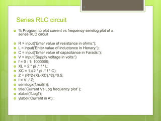
Series RLC circuit
 % Program to plot current vs frequency semilog plot of a
series RLC circuit
 R = input('Enter value of resistance in ohms:');
 L = input('Enter value of inductance in Henary:');
 C = input('Enter value of capacitance in Farads:');
 V = input('Supply voltage in volts:')
 f = 0 : 1: 1000000;
 XL = 2 * pi .* f * L;
 XC = 1./(2 * pi .* f * C);
 Z = (R^2-(XL-XC).^2).^0.5;
 I = V ./ Z;
 semilogx(f,real(I));
 title('Current Vs Log frequency plot' );
 xlabel('fLogf');
 ylabel('Current in A');
8
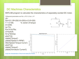
DC Machines Characteristics
MATLAB program to calculate the characteristics of separately excited DC motor.
%Required parameters are Ra, k, Rf, Vt, Ns, k, Vf
clc;
Ra=0.5 ;Rf=250;Vt=250;k=2;Vf=250;
T = 0:100; % vector of torque
If=Vf/Rf;
Ia=T/k;
Ea=Vt-Ia*Ra;
w=Ea/k/If;
N=w*60/2/pi;
plot(T,N)
xlabel('Torque')
ylabel('Speed in RPM')
title('Speed-Torque Curve')
plot(T,Ia)
xlabel('Torque')
ylabel('Armature Current')
study the characteristics of shunt and series DC motors
0 10 20 30 40 50 60 70 80 90 100
0
5
10
15
20
25
30
35
40
45
50
Torque
Armaturecurrent
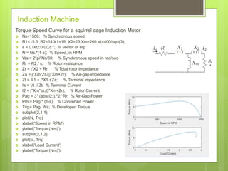
Induction Machine
Torque-Speed Curve for a squirrel cage Induction Motor
 Ns=1500; % Synchronous speed;
 R1=15.6 ;R2=14;X1=18; X2=23;Xm=260;Vt=400/sqrt(3);
 s = 0.002:0.002:1; % vector of slip
 N = Ns.*(1-s); % Speed, in RPM
 Ws = 2*pi*Ns/60; % Synchronous speed in rad/sec
 Rr = R2./ s; % Rotor resistance
 Zr = j*X2 + Rr; % Total rotor impedance
 Za = j*Xm*Zr./(j*Xm+Zr); % Air-gap impedance
 Zt = R1 + j*X1 +Za; % Terminal impedance
 Ia = Vt ./ Zt; % Terminal Current
 I2 = j*Xm*Ia./(j*Xm+Zr); % Rotor Current
 Pag = 3* (abs(I2)).^2.*Rr; % Air-Gap Power
 Pm = Pag.* (1-s); % Converted Power
 Trq = Pag/ Ws; % Developed Torque
 subplot(2,1,1)
 plot(N, Trq)
 xlabel('Speed in RPM')
 ylabel('Torque (Nm)')
 subplot(2,1,2)
 plot(Ia, Trq)
 xlabel('Load Current')
 ylabel('Torque (Nm)')
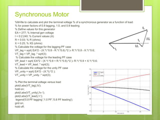
Synchronous Motor
%M-file to calculate and plot the terminal voltage % of a synchronous generator as a function of load
% for power factors of 0.8 lagging, 1.0, and 0.8 leading.
% Define values for this generator
EA = 277; % Internal gen voltage
I = 0:2:240; % Current values (A)
R = 0.03; % R (ohms)
X = 0.25; % XS (ohms)
% Calculate the voltage for the lagging PF case
VP_lag = sqrt( EA^2 - (X.*I.*0.8 - R.*I.*0.6).^2 )- R.*I.*0.8 - X.*I.*0.6;
VT_lag = VP_lag .* sqrt(3);
% Calculate the voltage for the leading PF case
VP_lead = sqrt( EA^2 - (X.*I.*0.8 + R.*I.*0.6).^2 )- R.*I.*0.8 + X.*I.*0.6;
VT_lead = VP_lead .* sqrt(3);
% Calculate the voltage for the unity PF case
VP_unity = sqrt( EA^2 - (X.*I).^2 );
VT_unity = VP_unity .* sqrt(3);
% Plot the terminal voltage versus load
plot(I,abs(VT_lag),'b');
hold on;
plot(I,abs(VT_unity),'k--');
plot(I,abs(VT_lead),'r:');
legend('0.8 PF lagging','1.0 PF','0.8 PF leading');
grid on;
hold off;
TransmissionLineVoltageRegulation
12
% INPUT THE LINE PARAMETERS
Z = input ('Enter Line Impedence, Z line: ');
Y = input ('Enter Line Admittance, Y line: ');
P = input ('Enter Recieving end Power, Pr: ');
VL = input ('Enter Recieving end Voltage, Vr: ');
PF = input ('Enter Recieving end Power factor, pfr: ');
% CALCULATION OF ABCD CONSTANTS
A=(1+Z*Y/2);
D=A;
B=Z;
C=Y*(1+Z*Y/4);
A1=acos(PF);
VR=VL/sqrt(3);
% CALCULATION OF RECEIVING END CURRENT
IR= P/(sqrt(3)*VL*PF);
IR=IR*(cos(A1)-j*sin(A1));
% CALCULATION OF SENDING END VOLTAGE
VS=A*VR+ B*IR;
VSA=abs(VS);
VSL=sqrt(3)*VSA;
% CALCULATION OF VOLTAGE REGULATION
VVRR=(VSA/abs(A)-VR)/VR;
VREGULATION = VVRR*100;
% CALCULATION OF SENDING END CURRENT
IS=C*VR+D*IR;
ISA=abs(IS);
% CALCULATION OF PHASE ANGLE
PA=angle(VS)*180/pi;
PB = angle (IS) *180/pi;
PS=(PA-PB)*pi/180;
PFS=cos(PS);
PS=sqrt(3)*ISA*VSL*PFS; % CALCULATION OF SENDING END POWER
EFFICIENCY=(P/PS)* 100; % CALCULATION OF EFFICIENCY
fprintf ('Efficiency is %dn', EFFICIENCY);
fprintf ('Voltage Regulation is %d n', VREGULATION);

MATLAB Scripts - Examples

  • 1.
    MATLAB Sample Scripts With ElectricalEngineering Applications Shameer A Koya
  • 2.
    Introduction  This lecturewe will do some practice on Basic MATLAB Scripts.  We will start with simple scripts and will discuss some electrical engineering applications.  More scripts including conditional statements will be discussed in the next lecture.  Please review lectures on basic input and output commands.
  • 3.
    Script 1 % Programto calculate Height of a Building from time a stone takes to reach the basement. % Use g=9.81and k=0.05 g=9.81; k=0.05; time= input (‘Enter the time taken: ‘); height=g*(time+(exp(-k*time)-1)/k)/k; disp(’Depth of well is ’) disp(depth) disp(’metres’)
  • 4.
    Script 2 % Programto calculate the BMI (body mass index) % Input your Height and Weight weight = input('Type your weight (kg): '); height = input('Type your height (m): '); bmi = weight / height^2; % Display the BMI fprintf('Your Body Mass Index is %fn", bmi);
  • 5.
    Script 3 % Programto calculate Electricity bill. w = input('Enter power of your device (in watts): '); h = input('Enter time (in hours): '); r = input('Enter electricity rate (in dollars per KWH): '); ec = w * h/1000 * r; disp(’Your Electricity bill is’) Disp(ec)
  • 6.
    Power transfer vsLoad resistance curve RL = 1:0.01:10; Vs = 12; Rs = 2.5; P = (Vs^2*RL)./(RL+Rs).^2; plot(RL,P) xlabel('Load resistance') ylabel('Power dissipated') 1 2 3 4 5 6 7 8 9 10 9 10 11 12 13 14 15 Load resistance Powerdissipated
  • 7.
    Curve fitting % Secondorder curve fitting %enter the input x and y vectors x = [0 .1 .2 .3 .4 .5 .6 .7 .8 .9 1]; y = [-.447 1.978 3.28 6.16 7.08 7.34 7.66 9.56 9.48 9.30 11.2]; n = 2; p = polyfit( x, y, n ) %Find the best quadratic fit to the data xi = linspace(0,1,100); yi = polyval(p, xi); % evaluate the polynomial plot(x,y,’-o’, xi, yi, ‘-’) xlabel(‘x’), ylabel(‘y = f(x)’) title(‘Second Order Curve Fitting Example’)
  • 8.
    Series RLC circuit % Program to plot current vs frequency semilog plot of a series RLC circuit  R = input('Enter value of resistance in ohms:');  L = input('Enter value of inductance in Henary:');  C = input('Enter value of capacitance in Farads:');  V = input('Supply voltage in volts:')  f = 0 : 1: 1000000;  XL = 2 * pi .* f * L;  XC = 1./(2 * pi .* f * C);  Z = (R^2-(XL-XC).^2).^0.5;  I = V ./ Z;  semilogx(f,real(I));  title('Current Vs Log frequency plot' );  xlabel('fLogf');  ylabel('Current in A'); 8
  • 9.
    DC Machines Characteristics MATLABprogram to calculate the characteristics of separately excited DC motor. %Required parameters are Ra, k, Rf, Vt, Ns, k, Vf clc; Ra=0.5 ;Rf=250;Vt=250;k=2;Vf=250; T = 0:100; % vector of torque If=Vf/Rf; Ia=T/k; Ea=Vt-Ia*Ra; w=Ea/k/If; N=w*60/2/pi; plot(T,N) xlabel('Torque') ylabel('Speed in RPM') title('Speed-Torque Curve') plot(T,Ia) xlabel('Torque') ylabel('Armature Current') study the characteristics of shunt and series DC motors 0 10 20 30 40 50 60 70 80 90 100 0 5 10 15 20 25 30 35 40 45 50 Torque Armaturecurrent
  • 10.
    Induction Machine Torque-Speed Curvefor a squirrel cage Induction Motor  Ns=1500; % Synchronous speed;  R1=15.6 ;R2=14;X1=18; X2=23;Xm=260;Vt=400/sqrt(3);  s = 0.002:0.002:1; % vector of slip  N = Ns.*(1-s); % Speed, in RPM  Ws = 2*pi*Ns/60; % Synchronous speed in rad/sec  Rr = R2./ s; % Rotor resistance  Zr = j*X2 + Rr; % Total rotor impedance  Za = j*Xm*Zr./(j*Xm+Zr); % Air-gap impedance  Zt = R1 + j*X1 +Za; % Terminal impedance  Ia = Vt ./ Zt; % Terminal Current  I2 = j*Xm*Ia./(j*Xm+Zr); % Rotor Current  Pag = 3* (abs(I2)).^2.*Rr; % Air-Gap Power  Pm = Pag.* (1-s); % Converted Power  Trq = Pag/ Ws; % Developed Torque  subplot(2,1,1)  plot(N, Trq)  xlabel('Speed in RPM')  ylabel('Torque (Nm)')  subplot(2,1,2)  plot(Ia, Trq)  xlabel('Load Current')  ylabel('Torque (Nm)')
  • 11.
    Synchronous Motor %M-file tocalculate and plot the terminal voltage % of a synchronous generator as a function of load % for power factors of 0.8 lagging, 1.0, and 0.8 leading. % Define values for this generator EA = 277; % Internal gen voltage I = 0:2:240; % Current values (A) R = 0.03; % R (ohms) X = 0.25; % XS (ohms) % Calculate the voltage for the lagging PF case VP_lag = sqrt( EA^2 - (X.*I.*0.8 - R.*I.*0.6).^2 )- R.*I.*0.8 - X.*I.*0.6; VT_lag = VP_lag .* sqrt(3); % Calculate the voltage for the leading PF case VP_lead = sqrt( EA^2 - (X.*I.*0.8 + R.*I.*0.6).^2 )- R.*I.*0.8 + X.*I.*0.6; VT_lead = VP_lead .* sqrt(3); % Calculate the voltage for the unity PF case VP_unity = sqrt( EA^2 - (X.*I).^2 ); VT_unity = VP_unity .* sqrt(3); % Plot the terminal voltage versus load plot(I,abs(VT_lag),'b'); hold on; plot(I,abs(VT_unity),'k--'); plot(I,abs(VT_lead),'r:'); legend('0.8 PF lagging','1.0 PF','0.8 PF leading'); grid on; hold off;
  • 12.
    TransmissionLineVoltageRegulation 12 % INPUT THELINE PARAMETERS Z = input ('Enter Line Impedence, Z line: '); Y = input ('Enter Line Admittance, Y line: '); P = input ('Enter Recieving end Power, Pr: '); VL = input ('Enter Recieving end Voltage, Vr: '); PF = input ('Enter Recieving end Power factor, pfr: '); % CALCULATION OF ABCD CONSTANTS A=(1+Z*Y/2); D=A; B=Z; C=Y*(1+Z*Y/4); A1=acos(PF); VR=VL/sqrt(3); % CALCULATION OF RECEIVING END CURRENT IR= P/(sqrt(3)*VL*PF); IR=IR*(cos(A1)-j*sin(A1)); % CALCULATION OF SENDING END VOLTAGE VS=A*VR+ B*IR; VSA=abs(VS); VSL=sqrt(3)*VSA; % CALCULATION OF VOLTAGE REGULATION VVRR=(VSA/abs(A)-VR)/VR; VREGULATION = VVRR*100; % CALCULATION OF SENDING END CURRENT IS=C*VR+D*IR; ISA=abs(IS); % CALCULATION OF PHASE ANGLE PA=angle(VS)*180/pi; PB = angle (IS) *180/pi; PS=(PA-PB)*pi/180; PFS=cos(PS); PS=sqrt(3)*ISA*VSL*PFS; % CALCULATION OF SENDING END POWER EFFICIENCY=(P/PS)* 100; % CALCULATION OF EFFICIENCY fprintf ('Efficiency is %dn', EFFICIENCY); fprintf ('Voltage Regulation is %d n', VREGULATION);