The document discusses generalized linear models (GLMs) and provides examples of logistic regression and Poisson regression. Some key points covered include:
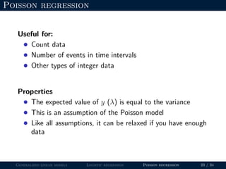
- GLMs allow for non-normal distributions of the response variable and non-constant variance, which makes them useful for binary, count, and other types of data.
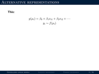
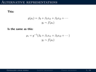
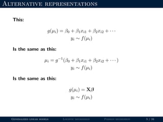
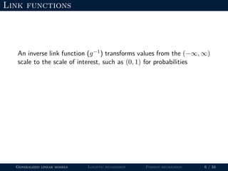
- The document outlines the framework for GLMs, including the link function that transforms the mean to the scale of the linear predictor and the inverse link that transforms it back.
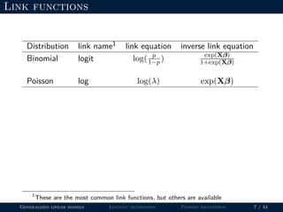
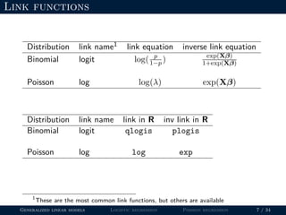
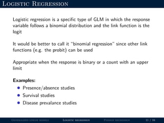
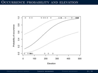
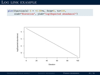
- Logistic regression is presented as a GLM example for binary data with a logit link function. Poisson regression is given for count data with a log link.
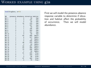
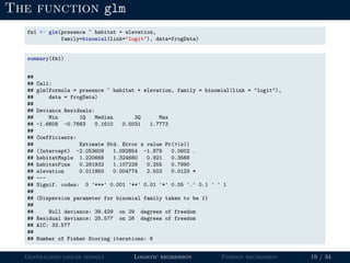
- Examples are provided to demonstrate how to fit and interpret a logistic


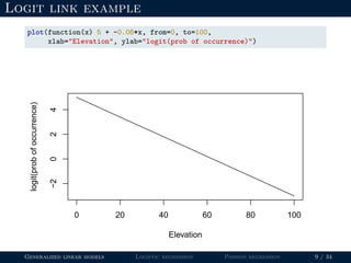
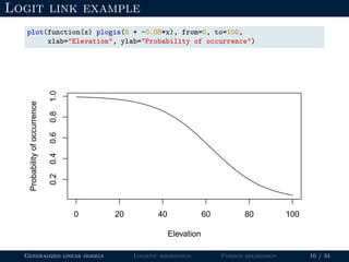
![Logit link example
beta0 <- 5
beta1 <- -0.08
elevation <- 100
(logit.p <- beta0 + beta1*elevation)
## [1] -3
Generalized linear models Logistic regression Poisson regression 8 / 34](https://image.slidesharecdn.com/lecture-glms-181109145655/85/Introduction-to-Generalized-Linear-Models-21-320.jpg)
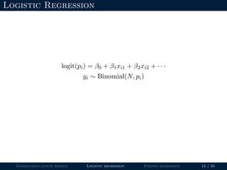
![Logit link example
beta0 <- 5
beta1 <- -0.08
elevation <- 100
(logit.p <- beta0 + beta1*elevation)
## [1] -3
How do we convert -3 to a probability?
Generalized linear models Logistic regression Poisson regression 8 / 34](https://image.slidesharecdn.com/lecture-glms-181109145655/85/Introduction-to-Generalized-Linear-Models-22-320.jpg)
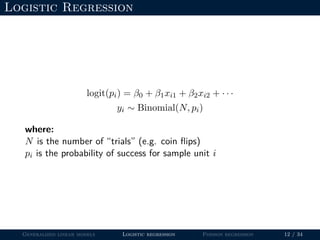
![Logit link example
beta0 <- 5
beta1 <- -0.08
elevation <- 100
(logit.p <- beta0 + beta1*elevation)
## [1] -3
How do we convert -3 to a probability? Use the inverse-link:
p <- exp(logit.p)/(1+exp(logit.p))
p
## [1] 0.04742587
Generalized linear models Logistic regression Poisson regression 8 / 34](https://image.slidesharecdn.com/lecture-glms-181109145655/85/Introduction-to-Generalized-Linear-Models-23-320.jpg)
![Logit link example
beta0 <- 5
beta1 <- -0.08
elevation <- 100
(logit.p <- beta0 + beta1*elevation)
## [1] -3
How do we convert -3 to a probability? Use the inverse-link:
p <- exp(logit.p)/(1+exp(logit.p))
p
## [1] 0.04742587
Same as:
plogis(logit.p)
## [1] 0.04742587
Generalized linear models Logistic regression Poisson regression 8 / 34](https://image.slidesharecdn.com/lecture-glms-181109145655/85/Introduction-to-Generalized-Linear-Models-24-320.jpg)
![Logit link example
beta0 <- 5
beta1 <- -0.08
elevation <- 100
(logit.p <- beta0 + beta1*elevation)
## [1] -3
How do we convert -3 to a probability? Use the inverse-link:
p <- exp(logit.p)/(1+exp(logit.p))
p
## [1] 0.04742587
Same as:
plogis(logit.p)
## [1] 0.04742587
To go back, use the link function itself:
log(p/(1-p))
## [1] -3
qlogis(p)
## [1] -3
Generalized linear models Logistic regression Poisson regression 8 / 34](https://image.slidesharecdn.com/lecture-glms-181109145655/85/Introduction-to-Generalized-Linear-Models-25-320.jpg)


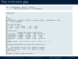


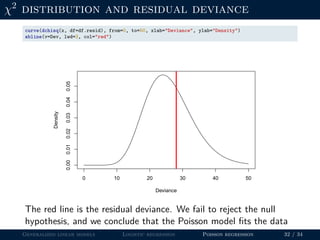
![Goodness-of-fit
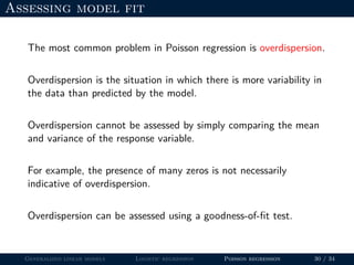
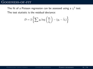
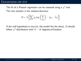
The fit of a Poisson regression can be assessed using a χ2 test.
The test statistic is the residual deviance:
D = 2 yi log
yi
ˆλi
− (yi − ˆλi)
If the null hypothesis is true (ie, the model fits the data), D should
follow χ2 distribution with N − K degrees-of-freedom.
N <- nrow(frogData) # sample size
K <- length(coef(fm2)) # number of parameters
df.resid <- N-K # degrees-of-freedom
Dev <- deviance(fm2) # residual deviance
p.value <- 1-pchisq(Dev, df=df.resid) # p-value
p.value # fail to reject H0
## [1] 0.3556428
Generalized linear models Logistic regression Poisson regression 31 / 34](https://image.slidesharecdn.com/lecture-glms-181109145655/85/Introduction-to-Generalized-Linear-Models-70-320.jpg)