Discrete Distribution.pptx

The Discrete
distribution
MBMG-7104/ ITHS-2202/ IMAS-3101/ IMHS-3101
@Ravindra Nath Shukla (PhD Scholar) ABV-IIITM

What is Probability Distribution?
Probability Distribution is a statistical function
which links or lists all the possible outcomes a
random variable can take, in any random
process, with its corresponding probability of
occurrence.

For example, if you roll a dice, the outcome is random (not
fixed) and there are 6 possible outcomes, each of which
occur with probability one-sixth.
Or A random variable X takes on a defined set of
values with different probabilities.
For example, if you toss a fair coin, there are 2 possible
outcomes head or tails, each of which occur with probability
1/2. The outcome of having head or tails is random (not
fixed).

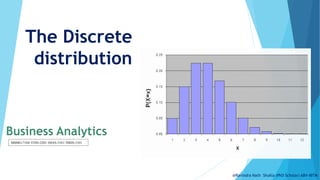
Mathematically :-
For example, if you toss a fair coin, two times -
Then sample Space for getting heads -
𝑆 = { 𝐻𝐻, 𝐻𝑇, 𝑇𝐻, 𝑇𝑇}
Let X = no. of heads., P(X) = probability of
coming heads.
T
4 possible outcomes
T
H
Probability Distribution
X Value Probability
0 1/4 = 0.25
1 2/4 = 0.50
2 1/4 = 0.25
T
T
H
H
H
0 1 2 X
Probability
0.50
0.25

PROBABILITY DISTRIBUTION OF A DISCRETE
RANDOM VARIABLE
Let us consider a discrete r.v. X which can take the possible
values x1, x2, x3,…, xn. With each value of the variable X, we
associate a number,
pi = P(X = Xi ) ; i = 1, 2,…, n
which is known as the probability of Xi and satisfies the
following conditions :
(i) pi = P(X = Xi ) ≥ 0, (i = 1, 2,…, n) …(1)
i.e., pi’s are all non-negative.

PROBABILITY DISTRIBUTION OF A DISCRETE
RANDOM VARIABLE
and
(ii) ∑ pi = p1 + p2 + … + pn = 1, …(2)
i.e., the total probability is one.
More specifically, let X be a discrete random variable and
define :
p (x) = P(X = xi)
such that p(x) ≥ 0 and ∑ p(x) = 1,

Requirements for the
Probability Distribution of a Discrete
Random Variable x
1. p(x) ≥ 0 for all values of x
2.  p(x) = 1
where the summation of p(x) is over all
possible values of x.
A probability function maps the possible values
of x against their respective probabilities of
occurrence, p(x)

Discrete example: roll of a die
x
p(x)
1/6
1 4 5 6
2 3
 
x
all
1
P(x)

Probability mass function (pmf)
x p(x)
1 p(x=1)=1/6
2 p(x=2)=1/6
3 p(x=3)=1/6
4 p(x=4)=1/6
5 p(x=5)=1/6
6 p(x=6)=1/6
1.0

Cumulative distribution function (CDF)
All random variables, discrete and continuous have
a cumulative distribution function (CDF).
Corresponding to any distribution function there is
CDF denoted by F(x), which, for any value of xi,
gives the probability of the event x≤ xi
Therefore, if f(x) is the PMF of x , then CDF is given
as
CDF for Discrete random variable

Cumulative distribution function
x
P(x)
1/6
1 4 5 6
2 3
1/3
1/2
2/3
5/6
1.0
x P(x≤A)
1 P(x≤1)=1/6
2 P(x≤2)=2/6
3 P(x≤3)=3/6
4 P(x≤4)=4/6
5 P(x≤5)=5/6
6 P(x≤6)=6/6

Mean for discrete distribution

Mean for discrete distribution
Example : - When throwing a normal die , let X be
the random variable defined by
X = the score shown on die
Probability distribution
X 1 2 3 4 5 6
P(x) 1/6 1/6 1/6 1/6 1/6 1/6
Or
𝐸(𝑋) = 1 ×
1
6
+ 2 ×
1
6
+ 3 ×
1
6
+ 4 ×
1
6
+ 5 ×
1
6
+ 6 ×
1
6
=
1
6
1 + 2 + 3 + 4 + 5 + 6 =
21
6
=
7
2
= 3.5

Variance for discrete distribution
Example : - for above example
X = the score shown on die
𝐸(𝑋2) = 12 ×
1
6
+ 22 ×
1
6
+ 32 ×
1
6
+ 42 ×
1
6
+ 52 ×
1
6
+ 62 ×
1
6
=
1
6
12 + 22 + 32 + 42 + 52 + 62
=
1
6
1 + 4 + 9 + 16 + 25 + 36 =
91
6

Variance for discrete distribution
Hence Variance
𝑉 𝑋 = 𝐸 𝑋2 − 𝐸 𝑋 2
=
91
6
−
7
2
2
=
35
12
= 2.916
Thus , standard deviation
𝜎 = 𝑉(𝑋) = 2.916
= 1.7076

Mean & Variance for discrete distribution
Example : - A company XYZ, estimates the net profit of a new
product it is launching, to be Rs. 3,000,000 during the first year if
it is successful, Rs. 1,000,000 if it is moderately successful and a
loss of Rs. 1,000,000. The company assigns the following
probabilities to first year prospectus for the product, successful:
0.15, moderately successful : 0.25, and unsuccessful : 0.60. What
are the expected value and standard deviation of first year net
profit for the product?
Hence Variance
𝑉 𝑋 = 𝐸 𝑋2 − 𝐸 𝑋 2
standard deviation 𝜎 = 𝑉(𝑋)

Common Probability Distribution

Uniform Distribution

Discrete example: roll of a die
x
p(x)
1/6
1 4 5 6
2 3
 
x
all
1
P(x)
𝑋 ~ 𝑈 𝑎, 𝑏
X~ U(1,6)
All outcomes has equal
probability

Bernoulli Distribution

Discrete example: True or Falls
𝑋 ~ 𝐵𝑒𝑟𝑛 𝑝
T
H

Binomial Distribution

Binomial Probability
The Binomial distribution is also know as the outcome of Bernoulli process.
A Bernoulli process is a random process in which :
a. The process is performed under the same conditions for a fixed and finite
number of trials, say, n.
b. Each trial is independent of other trials, i.e the probability of an outcome
for any particular trial is not influenced by the outcomes of the other
trials.
c. Each trial has two mutually exclusive possible outcomes, such as
"success" or "failure", "good or "defective", "yes" or "no", "hit" or
"miss", and so on. The outcomes are usually called success and failure
for convenience.
d. The probability of success, p, remains constant from trial to trial (so is
the probability of failure q, where, q = 1-p).

Binomial Probability
Characteristics of a Binomial Experiment
1. The experiment consists of n identical trials.
2. There are only two possible outcomes on each trial. We
will denote one outcome by S (for success) and the other
by F (for failure).
3. The probability of S remains the same from trial to trial.
This probability is denoted by p, and the probability of
F is denoted by q. Note that q = 1 – p.
4. The trials are independent.
5. The binomial random variable x is the number of S’s in
n trials.

Binomial Probability Distribution
!
( ) (1 )
! ( )!
x n x x n x
n n
p x p q p p
x x n x
 
 
  
 

 
p(x) = Probability of x ‘Successes’
p = Probability of a ‘Success’ on a single trial
q = 1 – p
n = Number of trials
x = Number of ‘Successes’ in n trials
(x = 0, 1, 2, ..., n)
n – x = Number of failures in n trials

Binomial Distribution
.0
.5
1.0
0 1 2 3 4 5
X
P(X)
.0
.2
.4
.6
0 1 2 3 4 5
X
P(X)
n = 5 p = 0.1
n = 5 p = 0.5

Binomial Probability Distribution
Example
3 5 3
!
( ) (1 )
!( )!
5!
(3) .5 (1 .5)
3!(5 3)!
.3125
x n x
n
p x p p
x n x
p


 

 


Experiment: Toss 1 coin 5 times in a row. Note
number of tails. What’s the probability of 3 tails?

Poisson Distribution

Poisson Distribution
1. Number of events that occur in an interval
• events per unit
— Time, Length, Area, Space
2. Examples
 Number of customers arriving in 20 minutes
 Number of strikes per year in the India.
 Number of defects per lot (group) of DVD’s

Characteristics of a Poisson Random Variable
1. Consists of counting number of times an event
occurs during a given unit of time or in a given area
or volume (any unit of measurement).
2. The probability that an event occurs in a given unit
of time, area, or volume is the same for all units.
3. The number of events that occur in one unit of
time, area, or volume is independent of the number
that occur in any other mutually exclusive unit.
4. The mean number of events in each unit is denoted
by .

Poisson Probability Distribution
Function

2 
p(x) = Probability of x given 
 = Mean (expected) number of events in unit
e = 2.71828 . . . (base of natural logarithm)
x = Number of events per unit
p x
x
( )
!

x
 
e–
(x = 0, 1, 2, 3, . . .)

Poisson Probability Distribution
.0
.2
.4
.6
.8
0 1 2 3 4 5
X
P(X)
.0
.1
.2
.3
0
2
4
6
8
1
0
X
P(X)
= 0.5
= 6
Mean
Standard Deviation
 


Poisson Distribution Example
At a departmental store, 72
customers arrive at store with a
rate of 72 customers per hour.
What is the probability for
arriving 4 customers in 3 minutes?
© 1995 Corel Corp.

Poisson Distribution Solution
72 Per Hr. = 1.2 Per Min. = 3.6 Per 3 Min. Interval
 
-
4 -3.6
( )
!
3.6
(4) .1912
4!
x
e
p x
x
e
p



 

Binomial Distribution Thinking Challenge
You’re a telemarketer selling service
contracts for XYZ co., You’ve sold
20 in your last 100 calls (p = .20). If
you call 12 people tonight, what’s
the probability of
A. No sales?
B. Exactly 2 sales?
C. At most 2 sales?
D. At least 2 sales?

Binomial Distribution Solution*
n = 12, p = .20
A. p(0) = .0687
B. p(2) = .2835
C. p(at most 2) = p(0) + p(1) + p(2)
= .0687 + .2062 + .2835
= .5584
D. p(at least 2) = p(2) + p(3)...+ p(12)
= 1 – [p(0) + p(1)]
= 1 – .0687 – .2062
= .7251

Thinking Challenge – Poisson distribution
You work in Quality Assurance for an
investment firm. A clerk enters 75
words per minute with 6 errors per
hour. What is the probability of 0
errors in a 255-word bond
transaction?
© 1984-1994 T/Maker Co.

Poisson Distribution Solution: Finding
*
 75 words/min = (75 words/min)(60 min/hr)
= 4500 words/hr
 6 errors/hr= 6 errors/4500 words
= .00133 errors/word
 In a 255-word transaction (interval):
 = (.00133 errors/word )(255 words)
= .34 errors/255-word transaction

Poisson Distribution Solution: Finding
p(0)*
 
-
0 -.34
( )
!
.34
(0) .7118
0!
x
e
p x
x
e
p



 

Discrete Distribution.pptx

Recommended

Recommended

More Related Content

What's hot

What's hot (20)

Similar to Discrete Distribution.pptx

Similar to Discrete Distribution.pptx (20)

More from Ravindra Nath Shukla

More from Ravindra Nath Shukla (12)

Recently uploaded

Recently uploaded (20)

Discrete Distribution.pptx