Hybridoma Technology ( Production , Purification , and Application )
1997 a+a 325-714-rhocas
1. Astron. Astrophys. 325, 714–724 (1997)
ASTRONOMY
AND
ASTROPHYSICS
Turbulence, mass loss and Hα emission by stochastic shocks
in the hypergiant ρ Cassiopeiae
Cornelis de Jager1 , Alex Lobel1,2, , and Garik Israelian2,3
1
SRON Laboratory for Space Research, Sorbonnelaan 2, 3584 CA Utrecht, The Netherlands
2
Astronomy Group, Vrije Universiteit Brussel, Pleinlaan 2, B-1050 Brussels, Belgium
3
Instituto de Astrofisica de Canarias, E-38200 La Laguna, Tenerife, Canary Islands, Spain
Received 17 February 1997 / Accepted 28 March 1997
Abstract. The hypergiant ρ Cas is known for its variable rate M1,max =1.06 to 1.08, a value that characterizes a fairly weak
of mass loss, with an average value of about 10−5 M y−1 , and shock-wave field.
the supersonic value for the line-of-sight component of the mi-
croturbulent velocity, about 11 km s−1 . Emission components Key words: stars: atmospheres – stars: supergiants – shock
in Hα suggest the presence of a thermally excited outer atmo- waves – turbulence – stars: mass loss
spheric region.
Since hydrodynamical turbulence in a stellar atmosphere
turns rapidly into a field of shock waves, and shock waves are
known to be able to initiate a stellar wind and heat stellar atmo-
spheric layers, we have tried to predict the rate of mass loss, the 1. The extreme properties of the hypergiant ρ Cas
microturbulent velocity component and the observed Hα pro-
file by assuming a stochastic field of shock waves. To that end The star ρ Cas (F8 Ia+ ) is a well-known example of the class
we adopted a Kolmogoroffian spectrum of shock waves, char- of hypergiants. Its luminosity classification (Ia+ ) means that its
acterized by only one parameter: the maximum Mach number spectral luminosity characteristics are more extreme than those
in front of the shocks: M1,max . Behind every shock a thin hot re- of class Ia. For ρ Cas the most notorious characteristics are the
gion originates. Spectroscopically, the thermal motions in these extreme luminosity, its irregular pulsations, the variable rate of
sheetlike regions cannot be distinguished from the stochastic mass loss, and the occurrence of displaced emission components
hydrodynamic (shock wave) motion component, and therefore in Hα. Beardsley (1961) was the first to notice that emission and
these hot regions add to the line broadening and will also con- he ascribed it to a circumstellar shell. In addition, the central
tribute to the observed ’microturbulence’. part of the line profile appears to be somewhat filled-in which
We find that it is indeed possible to explain the observed suggest excited upper chromospheric layers.
˙
rate of mass loss (we derived logM ≈ − 5 (M y−1 )), as well The semiregular small-amplitude variability in brightness
as the high value for the quasi-microturbulence (we calculated and radial velocity (Sargent 1961), have a typical brightness
12 km s−1 ). The hot sheets behind the shocks appear to be re- fluctuation of 0.2 mag, and an average ’quasi-period’ of 300 d.
sponsible for the observed ’microturbulence’; this thermal con- (Zsoldos & Percy 1991). Individual values of the quasi-period
tribution is much larger than that of the hydrodynamic (shock) range between 280 and 520 d. (Arellano Ferro 1985; Percy et al.
motions, which is only 0.4 to 0.5 km s−1 . Non-LTE calculations 1985; Sheffer & Lambert 1986). Lobel et al. (1994) have studied
of the Hα line profile show that the shocks, in association with the observed variations of brightness and radial velocity during
the observed time-dependent variation of Teff can reproduce as- 1970 and concluded that these variations cannot be ascribed to
pects of the variable emission in Hα. strictly radial pulsations.
Next to these small variations there are occasionally sudden
These three aspects of this star, viz. the observed rate of mass
larger jumps in brightness, often associated with considerable
loss, the observed supersonic ’microturbulence’, as well as the
changes of the spectral type. This latter phenomenon is not yet
Hα line profile can be simulated by one parameter only: viz.
fully understood, but it is usually ascribed either to larger-than-
usual pulsations with a stochastic character, or to excessive mass
Send offprint requests to: C. de Jager loss during relatively brief periods. Either phenomenon leads
Research Assistant of the Fund for Scientific Research - Flanders to the formation of an outwardly displaced photosphere (we
(Belgium) do not wish to use the term ’pseudophotosphere’), causing an
2. C. de Jager et al.:Turbulence, mass-loss and Hα emission by stochastic shocks in ρ Cas 715
Table 1. Data for ρ Cas one wavelength, into a field of shock waves. Hence, beyond a
level situated at an average wavelength above the convection
Effective temperature Teff = 7190 K layer, the atmospheric motion field must have turned into a field
Effective atmospheric accel. geff = 2.8 cm s−2 of shock waves.
Line-of-sight microturbulent
The general properties of the photospheric wave fields for a
velocity component ζµ = 11.1 km s−1
˙ number of super- and hypergiants, including ρ Cas, have been
Log of rate of mass loss log M = -5 ± 0.6 (M y−1 )
Log of luminosity logL/L = 5.7
derived by de Jager et al. (1991). Since the energies of the hy-
drodynamic waves are distributed over the wavelengths accord-
ing to a spectrum of turbulence the same must apply to the
field of shock waves. We will assume a Kolmogoroff spectrum,
increase of the stellar surface area and a consequent decrease of since some studies have shown that such a spectrum applies
the effective temperature. best to stellar photospheres (Dere 1989), and also because the
A matter that may need further investigation is the appear- Kolmogoroff spectrum is the only one that is theoretically justi-
ance of blueward displaced emission lines; in July 1960 Sar- fied for stellar atmospheric conditions. Once having made that
gent (1961) observed Ni i emission lines that were blueward assumption only one parameter is needed for defining all prop-
displaced with regard to single absorption lines, with vrad ≈25 erties of that spectrum. A suitable parameter is the maximum
km s−1 . More recent investigations show as a fairly general rule Mach number M1,max of the spectrum of shock wave energies.
that the radial velocity measured with the emission lines de-
viates only little from the system velocity (Sheffer & Lambert 2. Input data for the ’smooth background atmosphere’
1986). An example is the emission line Na i at 4527 cm−1 for
which a velocity of -49 km s−1 has been found (Lambert et Our input data for the ’smooth background atmosphere’ are
al. 1981). This value, combined with the system velocity (-42 based on an interpolated Kurucz model for the effective temper-
km s−1 ) yields a residual blueshift of only 7 km s−1 . The un- ature and acceleration of the star. A plane model was assumed,
certainty in these velocities is usually given as 1 km s−1 , but since the atmosphere of this star can be treated as being plane,
it may be larger due to blends. Lobel & de Jager (1997) have in spite of its extent, because of the star’s size relative to the
further studied the blueward displaced (≤10 km s−1 ) emission atmospheric thickness (de Jager 1981, p. 195). Onto this ’back-
components in neutral lines. They do not share the photospheric ground atmosphere’ we superpose the shock wave field. The
pulsations, and must be ascribed to a stationary detached shell numerous shocks are all followed by relatively thin regions of
at some ten to 20 stellar radii from the star. temperature enhancements. Therefore the addition of shocks to
Published values for the rate of mass loss were summarized the atmospheric model, in the subsequent phase of this inves-
by Lobel et al. (1994); they range between -6 and -3 (logarith- tigation, will on the average increase the average photospheric
mic), but the most reliable determinations range between -5.3 temperature, and integration of that new atmospheric model will
and -4.4. The scatter in the data is larger than the mean error of yield a higher effective temperature value than the input value.
a single unit weight mass loss determination, which is ±0.37 Therefore it is advisable to start with a lower value for the
(de Jager et al. 1988), and therefore seems to be real. A more input effective temperature, and our approach must be an itera-
recent value (Lobel et al. 1997) is -4.5. That value, however, tive one: after a first input of suitably chosen values for Teff and
seems to be related to a period of strong outward pulsational geff we derive the interpolated atmospheric (we call it hence-
motions. In this connection we should note that previously pub- forth ’smooth’ or ’smooth background’) model; then we add the
lished values for the log of the rate of mass loss, amounting to -2 shock wave spectrum, and calculate the stellar flux and effective
(Climenhaga et al. 1992) and -2.5 (Gesicki 1992) appeared not temperature for this new (’shocked’) atmosphere. Iteratively we
to be correct since they are based on a wrong interpretation of then search for those input data that yield Teff and geff values that
seemingly ’double’ lines that are actually absorption lines with agree best with the stellar data given in Table 1. After some trials
an emission core (Lobel and de Jager 1997). one quickly learns how to choose the input values in order to get
The atmospheric properties of the star have been determined rapid agreement with the observed stellar data. There is a slight
recently by Lobel et al. (1994). We give in Table 1 the data, that degree of ’feedback’, however: the precise values of the needed
we will use in this paper. The luminosity is taken from Gesicki input data appear to depend on the assumed shock strengths in
(1992). the atmosphere, hence on the input value M1,max of the shock
In this paper we will show that this set of parameters can spectrum. This means that the iterative procedure consists es-
be reproduced by assuming a photosphere in which a stochastic sentially of two weakly correlated acts: the choice of Teff and
field of shock waves is running outward. The reasons for as- geff , followed by the choice of M1,max . The first act should lead
suming a field of shock waves are, first that ρ Cas must have a to an effective temperature and effective acceleration that agree
subphotospheric convection region, wherein turbulence devel- with the observed values, and thereafter the second act should
ops, leading to outward running pressure waves. In addition it make two other observational quantities fitting: the rate of mass
is known that any field of hydrodynamic waves in a stellar at- loss and the microturbulent velocity component. (We do in this
mosphere transforms rapidly, i.e. within the time of one wave phase not yet consider the Hα line profile; this aspect will ap-
period, or after having traveled over a distance of the order of pear as a bonus from this investigation). Therefore, essentially
3. 716 C. de Jager et al.:Turbulence, mass-loss and Hα emission by stochastic shocks in ρ Cas
our problem reduces to the question whether one input value for
the shock spectrum can explain three observables: mass loss,
microturbulence, and the Hα line profile.
We next describe the way we calculated the ’smooth back-
ground model’. Before doing that we emphasize that it is not Fig. 1. A train of equal equidistant shocks in a homogeneous and
necessary to select a model in perfect radiative equilibrium, be- isothermal medium
cause the final (’shocked’) model anyway will not obey the ra-
diative equilibrium condition. The problem whether a shocked
atmosphere is in radiative equilibrium (we think it is not) has The wavelength of the shock is then z1 − z2 . We assume an
not been answered yet and formulating a decisive answer looks isothermal plasma (admittedly incorrect, but we think accept-
a formidable task. able in this phase); hence, we may neglect the energy equation.
We started with a Kurucz model of which the Teff and geff The equations of conservation of mass and momentum read:
values were closest to the expected final input data, and in that
model we took the temperature values for five logarithmically dρ/dt + d(ρv)/dz = 0. (1)
equally spaced optical depth values. A spline-type interpolation
function was drawn through the data points log(T (τ ))-log(Teff ), d(ρv)/dt + d(ρv 2 + P ) − ρg = 0 . (2)
which yields the function T (τ ) for the adopted Teff and geff val-
ues of this model, and - as we verified - also for the other models Introduce d/dt = d/dz×dz/dt = −U ×d/dz. Write further
that will be met in the course of this investigation. In doing this v = v/s, U = U/s, s2 = Γ1 ×P/ρ, where s is the velocity of
we based ourselves on the experience that photospheric models sound, and introduce z = z/H with the density scale height
have in good approximation the same (T (τ ) − Teff )-relation in H=RT /µg. Equations (1) and (2) then become dimensionless:
any restricted part of the (Teff ; geff ) plane.
The ’smooth background model’ is thereupon calculated as dlnρ/dz = [Γ1 (v − U )2 − 1/Γ1 ]−1 , (3)
follows. For an optical depth τRoss =10−6 we calculate start-
ing values for the pressure P and density ρ by solving for and
the known T (τ =10−6 ) value: P =geff ×10−6 /κRoss . The calcu-
lation is iterative because κ depends on P and ρ. Integration of
dv /dz = (dlnρ/dz )/(U − v ) . (4)
dP/dz=geff ×ρ and dτ /dz= κ×ρ (where we write κ for κRoss )
then yields the desired ’smooth background’ atmospheric model
We performed a number of numerical integrations and
as a function of the geometrical depth z and the optical depth
these yielded interpolation relations between the (dimension-
τRoss .
less) wavelength L/H, the velocity behind the shock v2 , and
For this atmosphere we also need to know the optical
the shock velocity U , all three quantities in dependence of the
and geometrical heights of the top level of the convection
parameters M and Γ. To give an example: for the wavelength
zone. This is done by searching for the depth level where
L/H a suitable representation reads:
∂(logT )/∂(logP )model =∂(logT )/∂(logP )ad . In deriving the last
quantity the influence of the ionization of H and He is taken into
account. L/H = Ap (Γ)×(M − 1) + Bp (Γ)×(M − 1)2 , (5)
with
3. Motion field between shocks
For the following we need relations between the wavelengths Ap (Γ) = aap + bap ×(Γ − 1.5) + cap ×(Γ − 1.5)2 (6)
of the shocks (i.e. the vertical distances between two consecu-
tive shocks), in dependence of the shock velocity amplitudes. Bp (Γ) = abp + bbp ×(Γ − 1.5) + cbp ×(Γ − 1.5)2 . (7)
To simplify the problem we introduce the following approxi-
mation. For any wavelength of the shocks we assume a one- We refrain from listing the values of the numerical quan-
dimensional train of identical, equidistant shocks, moving with tities aap through cbp . We have derived similar equations for
constant velocity into the vertical +z-direction, in a homoge- the relation between the relative velocity behind the shock v2
neous isothermal medium (Fig. 1). The velocity of propagation and the parameters M and Γ. A third set of interpolation equa-
is the ’shock velocity’ U , which can be derived from the shock tions applies to the dimensionless shock velocity U . We note
relations. that the quantity M is similar to, and will later be used for, the
The velocity profile is related to a similar density profile. We maximum Mach number M1 , but in the present context it is just
write for the log of the density and the shock velocity behind a formal parameter introduced in order to link the wavelength
the shocks logρ(z2 ) and v(z2 ). Mathematically, the problem is L/H, the velocity v2 and the shock velocity U with the values
then to calculate the functions logρ(z) and v(z) in a isothermal of Γ and M . By means of these equations we can also find the re-
medium, starting with the above boundary values and for de- lationship between the wavelength L/H and the dimensionless
creasing z, and also to find the point z1 where v(z1 ) = −v(z2 ). velocity v2 just behind the shock.
4. C. de Jager et al.:Turbulence, mass-loss and Hα emission by stochastic shocks in ρ Cas 717
4. Stochastic spectrum of shock waves which leads to new v2 (z) values. We will call these sorted shocks
the new shocks.
We next calculate the velocity distribution in the atmosphere
At this point shock physics enters into the picture. For each
defined by a Kolmogoroff spectrum of shock wave energies,
of the new shocks thus obtained we know the velocity amplitude
in which M1,max is the maximum Mach number in front of the
and from these values we derive the Mach numbers M1 in front
shocks. The wavelength corresponding to this Mach number is
of the shocks with (cf. Gail et al., 1990, Eq. (56))
called L0 . For such a spectrum the relationship between v2 or
v2 and L is given by
v2 = ((Θ − 1)/2Θ)×M1 ×s , (12)
2/3
v2 (L)/v2 (L0 ) = v2 (L)/v2 (L0 ) = (L/L0 ) . (8)
where Θ is the density ratio ρ2 /ρ1 . For deriving Θ we have to
The velocity variation between two equal shocks with a consider that ionization can be important at the temperatures and
wavelength L is a linear saw-tooth profile, with velocity v2 be- pressures involved. Therefore we use the generalized version
hind the leading shock and v1 in front of the trailing shock (as of the Rankine-Hugoniot relations (we abbreviate them as the
shown in Fig. 1). If we call this profile ΥL (z), then the mo- ’NDJCLA-equations’, Eq. (26) of Nieuwenhuijzen et al. 1993).
tion field (still without the contribution of the stellar wind) of a These equations can only be solved iteratively. For the first step
Kolmogoroff spectrum of shock waves is of iteration we used the classical Rankine-Hugoniot expressions
L0
Θ = ρ2 /ρ1 = ((γ + 1)M1 2 )/((γ − 1)M − 12 ) + 2) , (13)
vs (z) = (L/L0 )1/3 .ΥL (z + φ)dL , (9)
L1
where γ = cp /cv , calculated for the temperature and pressure
where φ is a phase with a value between 0 and L, which is gener- at the relevant level, taking ionization into account (for an ideal
ated by a random procedure. The introduction of this randomly gas γ = 5/3), and
distributed phase is necessary for simulating the real situation in
a stellar atmosphere. In any spectrum of turbulence the phases Φ = p2 /p1 = (2γM1 2 − γ + 1)/(γ + 1) . (14)
of the various wave components are distributed randomly. In
actual practice, the integration is replaced by a summation. The In order to proceed with the second approximation, we use
final velocity profile in the stellar atmosphere is then given by these quantities for deriving values of γH (cf. Nieuwenhuijzen et
al. 1993 for the definition of γH ) and Γ1 in front and behind the
v(z) = vs (z) + vw (z) , (10) shocks; these quantities are needed for the NDJCLA-relations.
Only then can the iteration proceed with the generalized NDJ-
where the value of the wind term vw is
CLA relations. The iterative derivation of M1 from v2 as outlined
˙
vw = M /4πr2 (z)ρ(z) . (11) here is straightforward and it appears to converge well. Fig. 3
(in Sect. 5) is a diagram, calculated for an exaggerated case,
˙
Here, M is the rate of mass loss; r(z) is the distance of the M1,max =1.5 in a giant-type atmosphere with loggeff =3 (hence,
point z from the stellar centre. We define the stellar radius by not a supergiant), and shows among other things the distribu-
τRoss =2/3. tion of the mass density logρ in a shocked model atmosphere of
When the velocity profile is known, one has to derive the this giant star, plotted against the geometrical depth scale. The
density- and temperature profiles in the shocked atmosphere. depth unit is an ’average scale height’. We note that the value
We discuss these matters here for the density and in the next M1,max =1.5 is for ρ Cas far too large, and also loggeff and the
section for the temperature. resulting rate of mass loss are by three orders too large but this
The point we make first is that shocks can accumulate. In the case demonstrates, better than smaller values, what we want to
actual numerical procedure the velocity vs (z) or v(z), according show.
to Eqs. (9) and (10) is given for a number of discrete z points; we Once M1 , v2 and the other parameters for the new shocks
used 250 points per average scale height interval. Because of the are known, it is also possible to find the shock velocity U =
integration (9) there appear a large number of shocks in the v(z) v1 +s×M1 , a quantity that is important for calculating the depth
curve. In order not to overload the program we deleted shocks variation of the temperature (next section). It should also be
with a velocity amplitude < 0.02s (s being the local speed of known for evaluating the importance of ’shock cannibalism’,
sound), which corresponds to the introduction of an artificial the process according to which larger and hence faster moving
lower limit for L1 ; we ascertained that the exclusion of these shocks overtake smaller, hence slower ones, and thus become
small shocks does not significantly change the overall results. In still larger and faster moving, etc., so that at the very, but in-
some cases it may happen, because of the discrete character of deed: very, long run only large shocks tend to remain. To give
the z axis, that two or more shocks add at a specific z point, and an example: for an atmosphere where the waves emerge from
thus one may even meet the situation (rarely, however) that one a subphotospheric convection region at τ ≈0.3 (the top of the
obtains shocks that are stronger than the largest input shock. The convection zone in a particular case) the fraction ∼0.9 of the
next step consists therefore of ’sorting’ the shocks according to shocks remains when the shocks have moved from that level
their z-values, taking into account their possible accumulation, until τ ≈0.1.
5. 718 C. de Jager et al.:Turbulence, mass-loss and Hα emission by stochastic shocks in ρ Cas
5. Temperature distribution in a shocked atmosphere
When the shock parameters such as the density- and pressure-
jumps behind the many shocks are known, the temperature is so
too, because of the equation of state. In the wake of every shock
the temperature excess with respect to the smooth temperature
distribution will decline radiatively. For the cooling time we
assume (Spiegel 1957)
τc = ρcv /16κσT 3 , (15)
where κ is the inverse of the photon free path, σ is Stefan-
Boltzmann’s constant and cv the specific heat per unit mass at
constant volume, calculated including the effects of ionization.
For κ we take the Rosseland absorption coefficient. The trans-
formation of the cooling time into a cooling distance goes via the
Fig. 2. Accumulation of post-shock high temperature regions. upper:
shock velocity U . This means that for an observer at a fixed point
high temperature; lower: low temperature
the temperature will rise at the shock to a value Tbackground +∆T ,
where ∆T is defined by the shock conditions, while it will de-
crease exponentially with time to the value Tbackground , with the zn . The temperature excess just behind the shock is TE (n), and
e-folding time defined by Eq. (15). Any instantaneous T (z)- the radiative cooling time of that shock is τn . At a point at a
picture of the whole atmosphere will show a number of shock- distance d1 behind shock no. 1 the temperature of the shocked
enhanced temperature jumps ∆T at the respective shocks (each atmosphere, due to the influence of shock no. 1 is (Fig. 2):
∆T -value being different, depending on the local shock condi-
tions; (cf. Fig. 2), followed to lower depths by an exponential T (z1 − d1 ) = Ts (z1 ) + TE (1) exp(−d1 /U1 τ1 ) . (16)
decline to Tbackground (while we know that Tbackground increases
with depth). The value of the exponential is in that case U/τc , Here, Ts (z1 ) is still the original ’smooth background tem-
where U is the shock velocity of the preceding shock. perature’, hence the interpolated Kurucz value. For the part of
This picture becomes more complicated at low tempera- the atmosphere behind the second and subsequent shocks, how-
tures, because the cooling time, which is short at high temper- ever, the ’background temperature’ at the position of the shocks
atures, increases for decreasing T -values. This poses a compu- is no longer the ’smooth background’ value but the accumulated
tational problem: suppose that an unshocked atmosphere has a effect of the temperature tails of preceding shocks as illustrated
low temperature, say 4000 K. Then τc L/U , where L is the in Fig. 2, lower part. If D2,1 is the distance between shocks nos.
distance between two successive shocks, and U the shock ve- 2 and 1, then the background temperature Tb (z2 ) at the position
locity. That means that in this case a next shock will occur in a of shock no. 2 is derived from Eq. (16) by writing z2 for z1 - d1
medium which still has a higher background temperature than and D2,1 for d1 . In general, the ’background’ temperature at the
Tbackground , and consequently the shock conditions will not be position of shock no. n is
determined by Tbackground , but by the enhanced temperature in n−1
the wake of the preceding shock. The effects of several wakes T (zn ) = Ts (zn ) + T E (m) exp(−Dn,m /Um τm ) , (17)
may thus accumulate as outlined in the cartoon in the lower m=1
part of Fig. 2. But this accumulation may go, as it appears, to
such an extent that the temperature in the initially low temper- where Dn,m is the distance between shocks n and m. Here,
ature part of the atmosphere would rise to such high values that any value of TE (m) is determined by the local thermodynamic
τ0 L/U . In that case, however, the above mentioned superpo- conditions at the location of shock no. m; the temperature at that
sition of temperature wakes would not occur; we would again position is influenced by more than just one preceding shock.
meet the situation of the upper part of Fig. 2, and the atmosphere The temperature just after shock no. n is found with the
would remain overall relatively cool, with only hot sheets af- above equation by summing up to m = n instead of to n − 1,
ter every shock. Sophisticated solutions should be considered realizing that Dm,m = 0. The temperature between shocks n and
for this non-linear feedback problem, but for the time being we n + 1 at a point z, at distances dn to shocks no. n is
are contented with a fairly simple approach. The most direct n
solution appears to be to start calculations far outside the at-
T (z) = Ts (z) + T E (m) exp(−dm /Um τm ) , (18)
mosphere, to eliminate boundary effects. To that end we choose
m=1
τstart =10−6 . From there on we number the shocks consecutively,
going inward. At a point at a distance dn behind shock no. n, for all positive dm values. In calculating τn for the nth shock
situated at the geometrical depth zn , we want to know the total with Eq. (15) the temperature in that point is derived from Eq.
temperature excess due to all shocks preceding that one. We (17). In calculating the values of TE (n) we used the modified
call Ts (zn ) the smooth background temperature at the position Rankine-Hugoniot relations (Nieuwenhuijzen et al. 1993).
6. C. de Jager et al.:Turbulence, mass-loss and Hα emission by stochastic shocks in ρ Cas 719
Fig. 3. Variation of logT (upper), logρ (middle) and v/s (bottom) in
a shocked atmosphere, plotted on a geometrical depth scale (z/<H>,
where <H> is an average scale height. The model is not for ρ Cas, Fig. 4. The shocked atmosphere for the model parameters from Fig.
but for a giant model with excessive shocks, viz. Teff =7319 K and 3, plotted here on a log(τR )-scale. The curves and ordinates are as in
geff =103 cm s−2 , and for M1,max =1.5. These gravity and maximum Fig. 3
Mach values are both far too high for the case of ρ Cas, but are in-
troduced to clearly show the features. The figure shows the run of the
three variables through a ’window’, bordered by z/<H>=2 and 7;
actual calculations were made for z/<H>=0 to 8. The log τR -values
corresponding to the two border-values of z/<H> are printed in the with T . The consequence is that the geometrically thin high-
lower corners. temperature sheets behind the shocks are fairly thick on a τ -
scale. We show this in Fig. 4, which corresponds to the same
model as the one shown in Fig. 3.
As may be understood, the summed-up temperature is too
low for the lowest n-values because of the neglect of the influ-
ence of shocks for τ ≤10−6 but deeper in the atmosphere, for This effect is important since one observes an atmosphere
larger n, this is no longer the case. Therefore, our procedure on a τ scale rather than on a geometrical scale. This makes the
yields unreliable results for very small optical depths, close to high-temperature effects of the atmosphere more pronounced
τ = 10−6 , but it appears to stabilize after a few units of logτ . In compared to the model plotted on a geometrical scale. Another
the atmospheric region of interest to us, above τ ∼10−3 , which aspect is that the accumulation of shocks causes a region of
is 3 τ -decades deeper, such a stable situation appears. enhanced temperature in the upper layers of the atmosphere.
Fig. 3 gives the variation of density, velocity and temperature This effect mimics a chromosphere.
along the geometrical (z/Haver ) scale, thus calculated, in the
exaggerated example of the shocked atmosphere presented in In our calculations we have artificially included the dissi-
Fig. 2. pation of shock energy, which is done by keeping the shock
For the model atmosphere thus obtained, values of the at- amplitude constant with depth. Without dissipation the ampli-
mospheric parameters should be derived. Hence we calculated: tude would increase with height (because of the decreasing den-
1. The effective temperature Teff . The computations were sity) but observations of the depth dependence of microturbu-
simplified by assuming ’gray’ absorption coefficients: κ(λ) = lence always show this to be practically constant with height (cf.
κRoss , but the error thus introduced was reduced to a second Achmad et al. 1991; Lobel et al. 1992, and references therein
order one by working strictly differentially (e.g. in our range of to earlier work). This is ascribed to the effect of dissipation. We
photospheric parameters the difference between the Teff values neglected the heating by shock dissipation, a process usually
between the real and gray atmospheres equals 415±10 K). held responsible for the formation of chromospheres in cool
2. The effective acceleration geff . This quantity was derived non-magnetic stars. But even with our approach the shocks al-
with geff =( T /µ)×(dz/dlnρ). It is clear that geff varies over ready produce effects that simulate a chromosphere, as will be
the depth of the atmosphere. For the time being we do not wish shown in Sect. 10. The additional effect of shock dissipation
to include that aspect, but we determine one value that may would enhance this phenomenon.
be considered representative for the line-forming part of the
atmosphere. Therefore we determined geff by taking the average Another consequence refers to the average velocity, ob-
over the atmospheric region between τRoss -values of 1 and 0.001. served in the stellar spectrum. While the average velocity of
the star is about zero when integrated over the z-scale, this is
not the case for the velocity plotted on a τ -scale. For that sit-
6. Shocked atmospheric model on a τ -scale
uation (Fig. 4) one would observe a net outstreaming velocity,
There is an interesting difference between the shocked at- even for the extreme and hypothetical case when the geometri-
mosphere plotted on a geometrical scale (z-variable) and the cally averaged velocity would be zero. In such a star, that is not
one plotted on an optical depth scale (τ -variable), because in losing mass, one would still observe an outstreaming velocity,
the temperature range corresponding to the atmospheres of which is of the order of s/3 in the case presented in Figs. 3 and
fairly cool stars the absorption coefficient κR increases strongly 4.
7. 720 C. de Jager et al.:Turbulence, mass-loss and Hα emission by stochastic shocks in ρ Cas
Fig. 6. The assumed contribution function CL (τR )
Fig. 5. Shocks initiate mass loss
also strong fluctuations in the temperature, even over relatively
7. Rate of mass loss
short distances. This observation brings us to the subject of
A system of sufficiently strong shock waves in an atmosphere the interpretation of the observed values of the ’microturbulent
in which the overall density decreases outwardly will lead to a velocity component’ ζµ .
net outflow of matter. This can be shown by integrating Methods for the diagnosis of stellar atmospheres and the
determination of the value of ζµ are all based on the implicit as-
∞
sumption of an atmosphere with a smooth T -variation. For such
ρv dz (19)
zstart an atmosphere equivalent widths of a number of lines of vari-
ous strengths are calculated, and ensuing systematic differences
over a system of equidistant equal shocks superimposed over between calculated and observed equivalent widths of lines are
an outward decreasing density profile (Fig. 5). As is clear from then used to generate new values for quantities such as e.g. ζµ .
this sketch there is a net outflow of matter. The point we make here is that quasi-stochastic temperature
This is evidently also the case in an atmosphere with a variations such as those shown in Figs. 3 and 4, will influence
stochastic distribution of shocks. Therefore shocks can initiate line profiles and their equivalent widths in a way similar to the
mass loss. stochastic hydrodynamic motions, and that it will be hard to
In calculating the rate of mass loss the question arises from distinguish observationally with conventional diagnostic tech-
what level in the atmosphere we should start the outward inte- niques between these two components.
gration of the integral (19). We decided to place the lower limit Therefore we derived a method for predicting the expected
zstart one scale height above the top of the convection zone. This value of the microturbulent velocity component ζµ for shocked
decision is based on the idea that the convection zone is the re- atmospheres, on the basis of these two causes for microturbulent
gion where hydrodynamic turbulence is generated and that only line broadening: hydrodynamic motions and temperature fluc-
above the convection zone, where waves run outward, these will tuations. We assume as known the variation of variables such
develop into shocks after having gone over a certain distance. as T (τ ), P (τ ), v(τ ), etc. in a shocked atmosphere. In deriving
For the latter quantity we took one scale height. expressions for the calculation of the expected value of ζµ we
Applied to the case of ρ Cas, we derived a rate of mass loss in further have to take two facts into consideration:
the range of the observed values 10−4.5 and 10−5.2 M y−1 . For 1. Not the whole range of optical depths of the atmosphere
the actual data reference is made to Sect. 9. We consider this contributes to the formation of a line. There is a contribution
as evidence that a field of shock waves of moderate strength function CL (Achmad et al. 1991), which varies from one line
can initiate stellar mass loss, at least in this type of hypergiant. to the other, but an average function can be given. We have
We add that we only claim that shocks initiate the process of derived such an average contribution function from Achmad et
mass loss, and not that they govern the velocity profile of the al. (1991) and show it in Fig. 6. As shown in that paper the
stellar winds in remote regions above the photosphere because contribution functions of different lines can vary, but plotted on
the shocks will be dissipated over a relatively short distance from a logτ scale the functions are more or less equal, apart from
the photosphere, while various other effects such as radiation a possible horizontal shift along the τ -axis; the most extreme
pressure may influence the velocity profile of the wind in the case being a downward shift over about one unit in the logτ
outer parts of the winds. scale. For the time being we use the diagram of Fig. 6, which
represents the average line-forming region.
8. Quasi-turbulence: the notion of microturbulence in a 2. Velocity- or temperature variations on very large geomet-
shocked atmosphere rical length scales do not contribute to microturbulent broaden-
ing. There is a microturbulent filter function Fµ (L) or Fµ (k),
Fig. 4 shows a shocked atmosphere on a logτ -scale. Not only where L is the wavelength of the motion field and k = L/2π is
the radial velocity varies in a semi-stochastic way, but there are the corresponding wave number. This filter function gives the
8. C. de Jager et al.:Turbulence, mass-loss and Hα emission by stochastic shocks in ρ Cas 721
The expected microturbulent velocity component is then
found from
∞
ζµ 2 = Ψc (α)2 dα. (24)
0
We stress that with the expressions above one finds the value of
the quasi-microturbulence as we may call it: it is the combined
contribution to line broadening by the short-scale variations of
the temperature and by those due to short-scale mass motions. If
one wishes to know the real hydrodynamic component of it (i.e.
the effect of mass motions only), the same expressions should
Fig. 7. The filter function Fµ (θ/L) for microturbulence be used with the exception that the last (the thermal) part of the
r.h.s. of Eq. (21) should be dropped. We have done so (see next
section), and while finding a quasi-turbulence of the order 12
fraction of the kinetic energy of the motion field at a certain
km s−1 , we find a hydrodynamic turbulence of only 0.5 km s−1 .
spatial wavelength that contributes to microturbulent broaden-
ing of a line. Stochastic motions on a short scale of heights will
fully contribute to the microturbulent broadening of lines; hence 9. Application to the case of ρ Cas
for motions with geometrical wavelength L λ, where λ is the We apply the above described algorithms to the hypergiant ρ
mean free path of the photons, we have Fµ =1. For motions with Cas. There are five input data: Teff , geff , the maximum Mach
L λ, one has Fµ =0, while Fµ takes intermediate values for number in front of the shocks M1,max , the rate of mass loss M , ˙
wavelengths in between. For the macroturbulent filter function and the luminosity L/L . These will define output values of
FM the reverse is true. ˙
Teff , geff , ζµ , vhydr and M .
The microturbulent filter function Fµ has been calculated We will show that only Teff and M1,max really matter. For
by De Jager & Vermue (1979) and was improved by Durrant the luminosity we exclusively used the observed value (cf. Ta-
(1979) (cf. also de Jager, 1981, pp. 47-49). It appears suitable ble 1), but we know there is an observational tolerance in this
to choose a dimensionless ordinate kθ or θ/L, where θ is the parameter, while, if other things remain equal, L(:)R2 (:)M 2 . ˙
optical scale height, defined by This proportionality is so obvious that it did not appear nec-
dz = θ dlogτ . (20) essary to play around with L, but in drawing conclusions the
L-dependence should be kept in mind.
The microturbulent filter function used by us is given in Fig.
In trial calculations we also found rapidly that the input
7, in which the abscissa is log(θ/L). ˙
value of M does not influence the results as long as the input
The further procedure is as follows. For defining the ’smooth ˙
value remains below logM <-2.5. This can be understood be-
atmospheric model’ we introduce the average temperature func- ˙ enters in the calculations is that it determines
cause the way M
tion <T (τ )> and the average velocity function <v(τ )> in the
the gradient of vwind . Such a gradient could introduce a contri-
shocked atmosphere. These ’smooth models’ were obtained by
bution to the resulting value of ζµ , but we found this not to be
taking the running averages of T (τ ) and v(τ ) over a distance
the case for ρ Cas. For this star this result stands at variance with
corresponding to one scale height. We thereupon introduce the
claims that the observed high microturbulent velocities would
function Φ(τ ), which describes the squared velocities due to the
2 be due to the gradient in the stellar wind velocity; cf. Lamers
v- and T -fluctuations (which contribute to ζµ ), with
& Achmad (1994). We think that their claim is due to the fact
8 (T (τ )− < T (τ ) >) that in their study use was made of fictitious lines that originate
Φ(τ ) = (v(τ )− < v(τ ) >)2 + . (21)
π×µ in the stellar wind, where the relatively strong wind gradient
may indeed simulate turbulent line broadening. The observed
Define next a function T rb(z) that describes which part of the
microturbulent velocities, used in our study (data that were also
atmosphere contributes to the observable microturbulent line
referred to by Lamers & Achmad), are all derived from spectral
broadening:
lines that are formed in the photosphere in the range of levels ap-
T rb(z) = Φ(τ (z))×CL (τ (z)). (22) proximately defined by the contribution function, shown in Fig.
Next the filterfunction must be introduced. Let F (1/α) be 6. At that level the density is sufficiently high to have vwind ≈0.
the filter function, where α is a dimensionless unit of length, We also found that there is no large variation possible in the
expressed in units of the average shale height Hav . We introduce input value of geff ; its value should be chosen only little (i.e.
a function F being the real part of the Fourier transform of 0.1) below the required (observational) value, which means
the field of hydrodynamic/thermal velocity fluctuations, and we that the shock wave field only slightly contributes to the effective
define the function Ψc (α) as acceleration.
∞
The input value of Teff should be chosen some 100 to 300 K
0
(F (z/α)×T rb(z)×F (1/α)dτ (z) below the desired (observational) value. This is so, because the
Ψc (α) = ∞ . (23)
0
F (z/α)×F (1/α)dτ (z) many hotter regions behind the shocks enhance the calculated
9. 722 C. de Jager et al.:Turbulence, mass-loss and Hα emission by stochastic shocks in ρ Cas
˙
Table 2. Course of iteration; log(L/L )=5.7 and logM =-6 Table 3. Integrations for a unique set of input data
Teff,in geff,in M1,max Teff,out geff,out ζµ vhydr logM˙ Teff,in geff,in M1,max Teff,out geff,out ζµ vhydr logM˙
(K) (K) (km s ) (km s ) (M y−1 )
−1 −1 (K) (K) (km s−1 ) (km s−1 ) (M y−1 )
6800 2.65 1.07 6930 2.65 11.7 0.6 -4.49 6910 2.63 1.06 7420 2.72 11.9 0.5 -4.80
6825 2.70 1.07 7110 2.82 11.7 0.5 -4.70 ditto ditto ditto 7160 2.67 11.9 0.5 -4.69
6830 2.68 1.06 6890 2.80 11.9 0.5 -4.72 ditto ditto ditto 7270 2.70 12.0 0.5 -4.91
6920 2.68 1.06 7150 2.86 11.7 0.4 -4.89
of the line profile can at times be partly or wholly filled-in by
flux and thus we may end up with a shocked photosphere with emission.
a somewhat higher effective temperature than the input value. We think that these aspects can be reconciled by the proper-
The only parameter that is really ’free’ is the remaining one: ties of a shocked atmosphere. The existence of many hot sheets
M1,max . behind the shocks may imply the appearance of emission com-
To show the course of the iterations we present in Table 2 ponents in the spectrum. To investigate this aspect, we have
the results of some trial calculations. The table gives the three calculated a Hα line profile for two shocked atmospheres char-
input values: Teff , geff and M1,max . We took in all calculations acterized by Teff =6991 K and geff =2.85, and by Teff =7197 K
˙
log (L/L )=5.7 (as in Table 1) and log M =-6, an arbitrary but and geff =2.9.
unimportant choise. Input data for the calculations are the shocked models with
the fluctuations of the temperature, electron density, mass den-
The gratifying result is that it appears indeed possible to re-
sity and velocity, all as functions of logm, where m is the mass
produce the observed values for the rate of mass loss as well as
above the layer of reference.
that of the high supersonic microturbulent velocity component,
To perform the non-LTE calculations use was made of cou-
the latter being a value that has always surprised observers.
pled equations of radiative transfer and of statistical equilib-
These results are obtained by assuming a spectrum of weak
rium, according to a method that has been described earlier by
shock waves, defined by a largest Mach number M1,max =1.06
Scharmer & Carlsson (1985). We used a computer code de-
to 1.07. The real hydrodynamical component of the motion field
scribed by Carlsson (1986). The atmospheric model was ap-
(= the fluctuations in v) is small, of the order of 0.4 to 0.6 km
proximated by a - slightly smoothed - model. Smoothing was
s−1 only. This result is compatible with current expectations: in
done in order to make the calculations not too cumbersome and
Kurucz’s models for stars like ρ Cas one would expect a maxi-
primarily to overcome convergence problems.
mum convective velocity of 1 km s−1 (cf. Kurucz 1996). The
hydrodynamical turbulence is expected to originate in the lower The theoretical results are given in Fig. 8, and compared
situated convection layer. The observed ’microturbulence’ of 11 with three observed profiles. The comparison shows that the
km s−1 would be fully incompatible with this maximum veloc- greatly variable aspect of the observed line profile is qualita-
ity, but the hydrodynamical component derived in this paper, tively reproduced by the calculations. The significant difference
agrees with it. between the two calculated line profiles is in part due to the dif-
ferent input values of Teff , but for another part it reflects the
Another aspect is that repeated calculations for one unique
stochastically variable character of the shock-wave field. This
set of input values yield different output data. This is because
is in our feeling an interesting new aspect, worthwhile a study in
of the introduction of random phases φ in the spectrum of tur-
more depth. We think to have shown by these trial calculations
bulence (Eq. (9)). Physically, this is correct, because also in a
that an atmosphere permeated by shocks, even by weak ones,
stellar atmosphere this would be the case: there is randomness
can yield drastic changes in the emergent Hα profile, particu-
in any spectrum of turbulent motions. For this reason it is not
larly when also the stellar temperature is changing. The shocked
sufficient to end the calculation with one seemingly aggreeing
atmosphere apparently succeeds in explaining the strong vari-
set of input parameters. There is a natural spreading in the output
ations in the profile. However, the asymmetry of the observed
data, which should be determined by a number of calculations
Hα profile is not reproduced by the calculations.
with the same set of input parameters. An example is shown in
For the time being we tentatively conclude that the general
Table 3, where such a set is reproduced. From a larger number
appearance and the strong variability of the Hα line profile could
of such calculations it was found that the scatter in ζµ and in
˙ be caused by a system of weak shocks in the atmosphere.
logM is 0.1 km s−1 and 0.07, respectively.
11. Conclusions
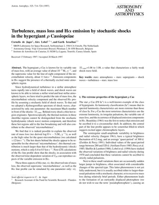
10. Calculated Hα line profile from a shocked atmosphere
Among the various remarkable aspects of the hypergiant ρ Cas
Spectral observations of ρ Cas occasionally show emission com- there are three that we try to explain in this paper: its supersonic
ponents of the subordinate line Hα and of strong resonance lines microturbulent velocity component, its fairly large rate of mass
like those of Ca ii. These emission peaks often show a blueward loss, and the variable appearance of the profile of Hα. We based
displacement by some 10 km s−1 . In addition, the central part our analysis on the feature that a system of hydrodynamic mo-
10. C. de Jager et al.:Turbulence, mass-loss and Hα emission by stochastic shocks in ρ Cas 723
Calculations show that a maximum shock strength
M1,max =1.06 to 1.08 appears to be fully capable of describ-
ing the observed rate of mass loss (10−5 M y−1 ) and the su-
personic value for the microturbulent velocity component (11
km s−1 ), while we find at the same time that the purely hy-
drodynamic component of shock-wave microturbulence is only
∼0.5 km s−1 , which is a much more reasonable value than the
extreme values found when taking the spectral data at their face
values. Microturbulence has often been called a ’fudge factor’
but such a qualification does not advance the physical under-
standing. We here claim that the observed ’microturbulent’ line
broadening is not caused by stochastic small-scale turbulent
motions (the classical notion of microturbulence) but by the
thermal motions in stochastically distributed high-temperature
sheets behind the many shocks.
Another result of this study is that the accumulation of high-
temperature sheets behind the many atmospheric shocks pro-
duces many relatively hot sheets, particularly in the outer layers
of the star (in deeper layers shocks do not so much lead to the
appearance of hot sheets because the shock heating is used for
ionizing the atmosphere behind the shocks, with small or zero
temperature enhancements). A non-LTE calculation of the ex-
pected profile of Hα shows that a shocked atmosphere is indeed
able to simulate the strongly variable displaced emission com-
ponents.
Finally, we have to refer to the approximations included in
the analysis. Most of them have been mentioned in passing. We
list them again:
We calculated the values of Teff assuming a gray atmosphere
(κ independent of wavelength); we have however tried to com-
Fig. 8. Calculated and observed line profiles of Hα. The calculated pensate that approximation by a strictly differential approach.
profile (upper panel; abscissa is velocity in km s−1 ) is for two in- The accumulation of the wakes of shocks and its influence
put models, defined by: Teff =6991 K and geff =2.85; Teff =7197 K and on the temperature structure of the atmosphere was handled in
geff =2.9; while also the variations in the outward velocity component a first-order way. More refined methods can be thought of.
have been taken into account. The observations (lower panel; abscissa:
˚
A) are (thick solid line): Nov. 30 ’91, courtesy O.R. Stahl; (thin solid The calculation of the ’standard’ v- and logρ-profiles in the
line): La Palma Observatory, Dec. 21 ’93 and (dashed line): La Palma shocks, as described in Sect. 3, was done assuming an isothermal
Observatory, July 25 ’94. situation, while we know that the gas behind the shocks is not
isothermal. There exist refined, but cumbersome methods for
calculating the velocity and density profiles behind shocks, but
for reducing computer time we did not want to use them in the
tions in the atmosphere of a star with a sufficiently extended present study.
atmosphere, such as ρ Cas, is likely to develop into a system of
shock waves. We have assumed that these shock waves follow We did not include the effect of pulsations, while recent
a Kolmogoroff spectrum of turbulence, defined by the maxi- observations suggest a certain degree of correlation between
mum Mach number M1,max in front of the shocks and we have strong pulsations and periods of enhanced mass loss.
examined the consequences of this assumption. These shocks
produce a net mass outflow component, hence they initiate mass
loss. The rate of mass loss can be calculated when the velocity- Acknowledgements. A.L. acknowledges financial support by the Fund
for Scientific Research - Flanders (Belgium) in 1995-97. G.I. wishes
and density-distributions in the shocked atmosphere are known.
to express his sincere thanks to Prof. J.P. de Greve in Brussels for
Furthermore, it appears that in a shocked atmosphere there is
his hospitality and to Dr. M. Carlsson for stimulating discussions. We
not only a quasi-stochastic distribution of velocities, but also thank O.R. Stahl for putting spectral observations at our disposal. Hans
of the temperature, the latter being due to the high-temperature Nieuwenhuijzen’s invaluable help in many computer problems is men-
sheets behind shocks. Both have their influence on the resulting tioned with thanks. We are obliged to Prof. Michael Grewing for a
microturbulent velocity component, but the latter much more number of very useful comments on a first draft. The suggestions from
than the former. an unknown referee are thankfully acknowledged.
11. 724 C. de Jager et al.:Turbulence, mass-loss and Hα emission by stochastic shocks in ρ Cas
References
Achmad L., de Jager C., Nieuwenhuijzen H., 1991, A&A 250, 445
Arellano Ferro A., 1985, MNRAS 216, 571
Beardsley W.R., 1961, ApJS 5, 381
Carlsson M., 1986, Ups. Astron. Obs. Rep., no. 33
Climenhaga J.L., Gesicki K., Smolinski J., 1992, in C. de Jager and
H. Nieuwenhuijzen (eds), Instabilities in evolved super- and hyper-
giants, North Holland, Amsterdam, p. 82
de Jager C., 1981, The Brightest Stars, Reidel, Dordrecht
de Jager C., Vermue J., 1979, Ap. Space Sci., 61, 129
de Jager C., Nieuwenhuijzen H., van der Hucht K.A., 1988, A&AS 72,
259
de Jager C., De Koter A., Carpay J., Nieuwenhuijzen H., 1991, A&A
244, 131
Dere K.P., 1989, ApJ 340, 599
Durrant C.J., 1979, A&A 73, 137
Gail H.P., Cuntz M., Ulmschneider P., 1990, A&A 234, 359
Gesicki K., 1992, A&A 254, 280
Kurucz R., 1996, in S.J. Adelman, F. Kupka, W.W. Weiss, (eds.): Model
Atmospheres and Spectrum Synthesis, ASP Conf. Ser. 108
Lambert D.L., Hinkle K.H., Hall D.N.B., 1981, ApJ 248, 638
Lamers H.J.G.L.M., Achmad L., 1994, A&A 291, 856
Lobel A., de Jager C., 1997, A&A, submitted
Lobel A., Achmad L., de Jager C., Nieuwenhuijzen H, 1992, A&A
256, 159
Lobel A., de Jager C., Nieuwenhuijzen H., Smolinski J., Gesicki K.,
1994, A&A 291, 226
Lobel A., Israelian G., de Jager C., Musaev F., Parker J. Wm., Mavro-
giorgou A., 1997 A&A, submitted
Nieuwenhuijzen H., De Jager C., Cuntz M., 1994, A&A 285, 595
Nieuwenhuijzen H., de Jager C., Cuntz M., Lobel A., Achmad L., 1993,
A&A 280, 195
Percy J.R., Fabro V.A., Keith D.W., 1985, JAAVSO, 14, 1
Sargent W.L.W., 1961, ApJ 134, 142
Scharmer G.B., Carlsson M., 1985, J. Comput. Phys. 59, 56
Sheffer Y., Lambert D.L., 1986, PASP 98, 914 and 99, 1272
Spiegel E.A., 1957, ApJ 126, 202
Zsoldos E., Percy J.R., 1991, A&A 264, 441
This article was processed by the author using Springer-Verlag L TEX
a
A&A style file L-AA version 3.