Abstract: The MEWMAChart is used in Process monitoring when a quick detection of small or moderate shifts in the mean vector is desired. When there are shifts in a multivariateControlCharts, it is clearly shows that special cause variation is present in the Process, but the major drawback of MEWMA is inability to identify which variable(s) is/are the source of the signals. Hence effort must be made to identify which variable(s) is/are responsible for the out- of-Control situation. In this article, we employ Mason, Young and Tracy (MYT) approach in identifying the variables for the signals. Keywords: Quality Control, Multivariate StatisticalProcessControl, MEWMA Statistic

1. Invention Journal of Research Technology in Engineering & Management (IJRTEM)
ISSN: 2455-3689
www.ijrtem.com Volume 1 Issue 2 ǁ March. 2016 ǁ PP 01-05
| Volume 1| Issue 2 | www.ijrtem.com | March 2016| 1 |
Detecting Assignable Signals Via Decomposition Of Newma Statistic
Nura Muhammad,1
Ambi Polycarp Nagwai,2
E.O.Asiribo,3
Abubakar Yahaya,4
P.G Student, Department of mathematics, Ahmadu Bello University, Zaria, Kaduna State, Nigeria1
Professor, Department of Statistics, University of Ewe, Ghana2
Professor, Department of Mathematics, Ahmadu Bello University, Zaria, Kaduna State, Nigeria3
Lecturer, Department of Mathematics, Ahmadu Bello University, Zaria, Kaduna State, Nigeria4
Abstract: The MEWMAChart is used in Process monitoring when a quick detection of small or moderate shifts in the mean vector is
desired. When there are shifts in a multivariateControlCharts, it is clearly shows that special cause variation is present in the Process,
but the major drawback of MEWMA is inability to identify which variable(s) is/are the source of the signals. Hence effort must be
made to identify which variable(s) is/are responsible for the out- of-Control situation. In this article, we employ Mason, Young and
Tracy (MYT) approach in identifying the variables for the signals.
Keywords: Quality Control, Multivariate StatisticalProcessControl, MEWMA Statistic.
1. INTRODUCTION
Nowadays, One of the most powerful tools in Quality Control is the StatisticalControlChart developed in the 1920s by
WalterShewharts, the ControlChart found wide spread use during World War II and has been employed, with various modifications,
ever since. Multivariate StatisticalProcessControl (SPC) using MEWMA statistic is usually employed to detect shifts. However,
MEWMAControlChart has a shortcoming as it can’t figure out the causes of the change. Thus, decomposition of𝑇2
is recommended
and aims at paving a way of identifying the variables significantly contributing to an out- of-Control signals.
1.1 Multivariate Controlfor Monitoring the ProcessMean:
Suppose that the Px1 random vectors𝑋1,𝑋2, − − − −,𝑋 𝑃each representing the P quality characteristics to be monitored, are
observed over a given period. These vectors may be represented by individual observations or sample mean vector. In 1992 lowery et
al developed the MEWMAChart as natural extension ofEWMA. It is a famous Chart employ to monitor a Process with a quality
characteristics for detecting shifts. The in ControlProcessmean is assumed without loss of generality to be a vector of zeros, and
covariance matrix∑.
TheMEWMAControl Statistic is defined as vectors,
𝑍𝑖=R𝑋𝑖+ (I-R)𝑍𝑖−1, i=I, 2, 3---------
Where 𝑋0=0, andR=diag(𝑟1, 𝑟2,−−−−−, 𝑟𝑝), 0≤𝑟𝑘 ≤ 1, i =1, 2, 3, -------, p
The MEWMAChart gives an out ofControl signals when
𝑇𝑘
2
= 𝑍𝑖
𝑡
∑𝑧𝑖
−1
𝑍𝑖−1 > ℎ
Where ℎ>0is chosen to achieve a specified in Control ARL and∑ 𝑧𝑖 isthe covariance matrix of 𝑋0 given by∑ 𝑧𝑖=
𝜕
2−𝜕
∑,under equality
ofweights of past observation for all P characteristics.
The UCL=.
𝑛−1 𝑝
𝑛−𝑝
. 𝐹∝,𝑃, 𝑛−𝑝 . if at least one point goes beyond upper Control limits the Process is assumed to be out of Control.
The initial value 𝑍0 is usually obtained as equal to the in-Control mean vector of the Process. It is obvious that if R=I, then the
MEWMAControlChart is equivalent to the Hotelling’s𝑇2
Chart.
The value ofhis calculated by simulation to achieve a specified in Control ARL. Molnau et al presented a programmed that
enables the calculation of the ARL for the MEWMA when the values of the shifts in the mean vector, the Control limit and the
smoothing parameter are known Sullivan and Woodall(5) recommended the use of a MEWMA for the preliminary analysis of
multivariate observation. Yumin(7) propose the construction of a MEWMA using the principal components of the original variables.
Choi et al(2). Proposed a general MEWMAChart in which the smoothing matrix is full instead of one having only diagonal. The
performance of this Chart appears to be better than that of the MEWMA proposed by Lowry et al (3). Yet et al (6). Introduced a
MEWMA which is designed to detect small changes in the variability of correlated Multivariate Quality Characteristics, while Chen et
al (1)proposed a MEWMAControlChart that is capable of monitoring simultaneously the Process mean vector and Process covariance
matrix. Runger et al (4). Showed how the shift detection capability of the MEWMA can be significantly improved by transforming the
original Process variables to a lower dimensional subspace through the use of the U-transformation.
1.2 The MYT Decomposition
The 𝑇2
statistic can be decomposed into P-orthogonal components (Mason, Tracy and Young) for instance, if you have P-
variates to decompose, the procedure is as follows:

2. Detecting Assignable Signals Via Decomposition Of Newma Statistic
| Volume 1| Issue 2 | www.ijrtem.com | March 2016| 2 |
𝑇2=𝑇1
2
+ 𝑇2.1
2
+ − − − + 𝑇𝑃.1,2,−−−−−−−𝑃−1−−−−−−−−−−−−−−
2
(1)
The first term is an unconditional𝑇2
, decomposing it as the first variable of the
𝑇1
2
=
𝑍1
2
𝑆1
2 ------------------------------------------------------------------ (2)
Where 𝑍1 and 𝑆1 is the transform X-variable and standard deviation of the variable 𝑍1 respectively.𝑇𝐽
2
Will follow an F-Distribution
which can be used as upper Control Limit
𝑇𝑗
2
=
𝑍𝑗
2
𝑆𝑗
2 ∽
𝑛˖1
𝑛
𝐹∝,1,𝑛−1.
Taking a case of three variables as anexample, it can be decomposed as,
𝑇1
2
+ 𝑇2.1
2
+𝑇3.12
2
𝑇1
2
+𝑇3.1
2
+𝑇2.13
2
𝑇2
2
+ 𝑇1.2
2
+𝑇3.12
2
----------------------------------------------------------- (3)
𝑇2
2
+𝑇3.2
2
+𝑇1.23
2
𝑇3
2
+ 𝑇1.3
2
+𝑇2.13
2
𝑇3
2
+ 𝑇2.3
2
+𝑇1.23
2
It is obvious that with increase in the number of variables, the number of terms will also increase drastically which makes the
computation become troublesome.
2. Illustration
In this section, we intend to demonstrate by way of example, how an assignable signal could be detected, the data that was
used for the purpose of the research was collected from a Portland cement company in Lagos, Nigeria. The data consistsof
temperature from a boiler machine in which twenty five observations were taken under different temperatures. The covariance matrix
given below was obtained from the data.
54 0.958 20.583
0.958 4.84 2.963
20.583 2.963 22.993
Having obtained the covariance matrix, the computation of 𝑇2
statistic was done using MATLAB computer package and the values
obtained for each of the twenty five observations are as shown in the table.
TABLE 1:
Computation ofMEWMA Statistic for individual observation
NNoo ooff oobbsseerrvvaattiioonn TTkk²² UUCCLL == HH
11 1100..6699 ** ** 99..9988
22 99..7700
33 55..6677
44 44..1144
55 00..9955
66 11..4400
77 00..6611
88 11..3377
99 99..6611
1100 77..5555
1111 44..7766
1122 22..3377
1133 11..4477
1144 44..2200
1155 22..6611
1166 22..7755
1177 33..7722
1188 00..4488
1199 11..5555
2200 11..7777
𝑇2
=

3. Detecting Assignable Signals Via Decomposition Of Newma Statistic
| Volume 1| Issue 2 | www.ijrtem.com | March 2016| 3 |
2211 00..4411
2222 00..7700
2233 33..0011
2244 33..0099
2255 55..9922
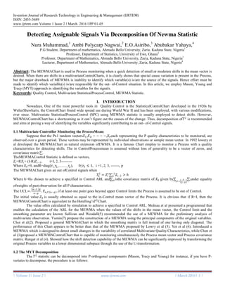
Below is the graph of MEWMA statistic for individual observation, where the individual 𝑇2
values were plotted against the number of
observations, and the dotted line represents the Control limit.
Figure 1: Chartof MEWMA Statistic
As it can be seen from the graph as well as the computation of 𝑇2
statistic in the table above, it is clear that observation (1) is
out of Control, as such, in order to detect the assignable signal, we consider observation( 1), and the procedure is as follow:
𝑇𝑘
2
= 𝑍𝑖
1
∑ 𝑧𝑖
−1
𝑍𝑖−1, ∑ 𝑧𝑖=
𝜕
2−𝜕
.Therefore,
𝑇1
2
𝑍1, 𝑍2, 𝑍3 = −1.8 0.244 − 1.192
0.2629 0.0999 −0.02482
0.0999 2.0978 −0.3598
−0.02482 −0.3598 0.6679
−1.8
0.244
−1.192
= 9.98
UCL =
𝑛−1 𝑝
𝑛−𝑝
. 𝐹∝,𝑃, 𝑛−1 = 9.98
The above result shows that the𝑇2
overall is significant, as such we now decompose 𝑇2
into its orthogonal components to be able to
determine which among the three variables contribute most as well as responsible to the out of Control signals. Therefore, from
equation (3) above, where for p=3 we had 18 component of 𝑇2
with different equation each is produce the same overall𝑇2
. The
calculation for each component as well as the sum of each term is as follows:
Starting with unconditional terms as given below:
𝑇1,
2
=
𝑍1
2
𝑆11
=
(−1.8)²
54
= 0.06, 𝑇2
2
=
𝑍2
2
𝑆22
=
(0.244)²
4.84
= 0.012,
and, 𝑇3
2
=
𝑍3
2
𝑆33
=
(−1.192)²
22.993
= 0.062
Therefore, the UCL for unconditional terms is computed as follows:
UCL =
𝑛+1
𝑛
. 𝐹∝,1,𝑛−1
It is show that all the variable𝑠𝑇1
2
, 𝑇2
2
and 𝑇3
2
are in Control since they are less than the UCL of the unconditional terms

4. Detecting Assignable Signals Via Decomposition Of Newma Statistic
| Volume 1| Issue 2 | www.ijrtem.com | March 2016| 4 |
To compute the conditional terms we proceed as follows:
𝑇3.12
2
= 𝑇2
𝑍1 𝑍2 𝑍3 − 𝑇2
𝑍1 𝑍2
To obtain𝑇2
𝑍1 𝑍2 𝑍3 we petition the original estimate ofZ- vector and covariance structure to obtain the Z- vector and cov- matrix
of the Sub vector 𝑍2
= 𝑍1 𝑍2 . the corresponding partition given as
∑ =
54 0.958
0.958 4.54
,2 Z2
=
−1.8
0.244
𝑇2
= (−1.8, 0.244) 54 0.958
0.958 4.54
−1
−1.8
0.244
= 0.0758
𝑇2.1
2
= 𝑇2
𝑍1 𝑍2 𝑍3 − 𝑇2
𝑍1 𝑍2 = 10.69 – 0.06=0.0158
𝑇3.1=
2
𝑇2
𝑍1 𝑍2 𝑍3 – 𝑇2
𝑍1 𝑍3 =10.69 – 0.0758= 10.61
From the above we can now obtain
𝑇2
= 𝑇2
𝑍1 𝑍2 𝑍3 = 𝑇1
2
+𝑇2.1
2
+𝑇3.12
2
= 0.06 + 0.00158 + 10.61 = 10.69
Since the first two terms have small value implies that the signal is contained in the third terms
𝑇3.12
Next, we check whether there is signal in 𝑍1 𝑍2 , we partition original observation into two groups 𝑍1 𝑍2 and 𝑍3
Having computed the value of 𝑇2
𝑍1 𝑍2 = 0.0758, then we compare it with UCL = 𝑍1 𝑍2 <7.4229. We conclude that, there is no
signal present in 𝑍1 𝑍2 components of the observation Vector. Hence it’s implies that the signal lies in the third component.
Therefore, the above decomposition consider MYT so as to illustrate it’s ensure that whichever MYT decomposition terms. Yield the
same overall 𝑇2
as follows:
𝑇1
2
+ 𝑇2.1
2
+𝑇3.12
2
= 0.06 + 0.0158 + 10.61 =10.69
𝑇1
2
+𝑇3.1
2
+𝑇2.1 3
2
=0.06 + 0.0169 + 10.6131 = 10.69
𝑇2
2
+ 𝑇1.2
2
+𝑇3.12
2
= 0.012 + 0.0639 + 10.6141 = 10.69
𝑇2
2
+𝑇3.2
2
+𝑇1.23
2
=0.012 + 0.2881 + 10.3899 = 10.69
𝑇3
2
+ 𝑇1.3
2
+𝑇2.13
2
= 0.062 + 0.0149 + 10.6131 = 10.69
𝑇3
2
+ 𝑇2.3
2
+𝑇1.23 =
2
0.062 + 0.238 + 10.3899 = 10.69
With the aids of the result decomposedabove; the value of each term of the decomposition was compared to the respective critical
value as indicated in the table below:
Table: 2
MYT Decomposition Component for Observation (1)
CCoommppoonneenntt VVaalluuee CCrriittiiccaall vvaalluuee
?? ??11
22 00..0066 44..44330044
?? ??22
22 00..001122 44..44330044
?? ??33
22
00..006622 44..44330044
?? ??11..22
22 00..00663399 77..44222299
?? ??11..33
22
00..00114499 77..44222299
?? ??22..11
22 00..00115588 77..44222299
?? ??33..11
22
00..00116699 77..44222299
?? ??22..33
22
00..22888811 77..44222299
?? ??33..22
22
00..22888811 77..44222299
?? ??11..2233
22
1100..3399 1100..3388 ** **
?? ??22..1133
22
1100..6611 1100..3388 ** **
?? ??33..1122
22
1100..6611 1100..3388 ** **
From the above table, we discovered that 𝑇1.23
2
+ 𝑇2.13
2
+𝑇3.12
2
have significant values, which means there is a problem in the
conditional relation between𝑍1, 𝑍2and𝑍3 we may conclude that the conditional relation between𝑍1, 𝑍2and 𝑍3 are potential causes of
the shifts. To verify the problems, we remove each conditional relation from the vector of observation (1) and check whether the sub
vector signals or not.
𝑇2
-𝑇1.23
2
= 10.69 − 10.38 = 0.31 < 10.69
𝑇2
-𝑇2.13
2
= 10.69 − 10.38 = 0.31 < 10.69
𝑇2
-𝑇3.12
2
=10.69-10.38=0.38<10.69
The outcomes Shewthat, the sub vector is insignificant. The meaning of significant value of 𝑇1.23
2
is that 𝑍1conditioned by
𝑍2 and 𝑍3 deviates from the variables relation pattern established from the historical data set. Similarly, and vice-versa for the
conditioned of𝑍1, 𝑍2and 𝑍3 were detected as being responsible sources for the assignable causes in observation (1).

5. Detecting Assignable Signals Via Decomposition Of Newma Statistic
| Volume 1| Issue 2 | www.ijrtem.com | March 2016| 5 |
3. CONCLUSION
In thisarticle, we were able to point out how 𝑇2
MEWMA Statistic decomposition Procedure was employed to detect
assignable signal. Broadly speaking, ControlCharts are used so as to be able to distinguish between assignable and natural causes in
the variability of quality goods produce. With regards to this, verifying which combination of quality characteristics is responsible for
the signal. Therefore the ControlChartplays a key role to inform us the appropriate next line of action to be taken in order to enhance
the quality.
REFRENCES
[1.] Chen GM, Cheng SW, Xie HS. A New Multivariate ControlChart for monitoring both location and dispersion.
Communications in Statistics-Simulation and Computation 2005; 34:203-217
[2.] Choi S, Lee Hawkins DM. A general multivariate exponentially weighted moving average ControlChart.Technical Report
640, School of statistics, University of Minnesota, May 2002
[3.] Lowry, C.A., Woodall, W.H., Champ, C.W. and Rigdon, S.E. (1992) a Multivariate Exponentially Weighted Moving
Average ControlChart. Technometrics, Vol. 34(1), pp. 46-53
[4.] Runger GC, Keats JB, Montgomery DC, Scranton RD. Improving the performance of a Multivariate EWMA ControlChart.
Quality and Reliability Engineering International 1999, 15:161-166
[5.] Sullivan JH. Woodall W.H. Adopting ControlCharts for the preliminary Analysis of Multivariate Observation.
Communications in Statistics-Simulation and Computation 1998; 29: 621-632
[6.] Yeh AB, Lin DKJ, Zhou H, Venkataramani C.A multivariate exponentially weighted moving average ControlChart for
monitoring Process variability. Journal of Applied Statistics 2003; 30: 507-536
[7.] Yumin L.An improvement for MEWMA in multivariate ProcessControl. Computers and Industrial Engineering 1996;
31:779-781
APPENDIX I
Boiler Temperature Data
NN00..ooff oobbsseerrvvaattiioonn XX11 XX22 XX33
11 550077 551166 552277
22 551122 551133 553333
33 552200 551122 553377
44 552200 551144 553388
55 553300 551155 554422
66 552288 551166 554422
77 552222 551133 553377
88 552277 550099 553377
99 553333 551144 552288
1100 553300 551122 552288
1111 553300 551122 554411
1122 552277 551133 554411
1133 552299 551144 554422
1144 552222 550099 553399
1155 553322 551155 554455
1166 553311 551144 554433
1177 553355 551144 554422
1188 551166 551155 553377
1199 551144 551100 553322
2200 553366 551122 554400
2211 552222 551144 554400
2222 552200 551144 554400
2233 552266 551177 554466
2244 552277 551144 554433
2255 552299 551188 554444
TToottaall 1133112255 1122883399 1133447733
AAvveerraaggee 552255 551133..3366 553388..9922