2. 294 J.-N. Pan et al. / Expert Systems With Applications 62 (2016) 293–301
neighboring stages and the residual EWMA and CUSUM control
charts for each stage can be constructed accordingly. Then, we pro-
pose a new Overall Run Length (ORL) for evaluating the overall
detecting ability of new control chars for multistage manufactur-
ing systems. In addition, the cumulative density function (CDF) of
ORL is derived and its correctness has also been confirmed. Subse-
quently, a simulation study is conducted to explore various combi-
nation of control parameters for multistage residual control charts
when the average of Overall In-Control Run Length (AOIRL) is fixed
at 370 (i.e. we fix the type I error rate of the overall multistage sys-
tem at 0.27%). Once the AOIRL is fixed at 370, the average of Over-
all Out-of-Control Run Length (AOORL) is used to evaluate the de-
tecting ability of multistage residual control charts when the mul-
tistage system is out of control. Furthermore, a sensitivity analysis
is performed to explore the effect of AOORL on the detecting abil-
ity of multistage residual control charts when the number of stage
increases. Finally, a numerical example with oxide thickness mea-
surements of a three-stage silicon wafer manufacturing process is
used to illustrate the usefulness of our proposed multistage resid-
ual control charts in the Phase II monitoring.
2. Literature review
2.1. Monitoring the process quality for multistage systems
In a multistage manufacturing system, the quality characteris-
tics of interest are often highly dependent. To monitor and diag-
nose the multistage manufacturing system, Zhang (1984), Zhang
(1987), Zhang (1990) & Zhang (1992) proposed the Cause-Selecting
Charts (CSCs). The advantage of this method is that once an out-
of-control signal or a special cause occurs in the process, it can
effectively distinguish which stage/subprocess is out of control.
To monitor quality of a process with multivariate variables,
Hawkins (1991) proposed Shewhart and CUSUM control charts
based on regression-adjusted variables. He further proposed the
concept of group charts. Tsung & Xiang (2004) proposed Group
EWMA Chart with One-Step Forecasting Errors (OFSE) combining
quality characteristics from multistage manufacturing system into
a single stage control statistic. The control statistic is defined as:
MZj = max
1≤k≤N
Zk,j
where Zk, j is the EWMA statistics of jth OFSE. Even though this
control statistics combine the multistage control charts into a sin-
gle stage control chart, it doesn’t preserve the structure of CSCs
and thus loses the advantage of using CSCs. Moreover, it is not
easy to trace back to the root stage where the subprocess is out
of control.
Yang & Yang (2006) considered a two-step process in which
the observations X in the first step can be modeled as an auto-
correlated autoregressive model of order 1 (AR(1)) model and the
observations in the second step Y can be modeled as a transfer
function of X. The AR(1) model they used can be written as:
Xt = (1 − φ)ξX + φXt−1 + at , t = 1, 2, . . .
where ξX is the process mean of the first step, φ is the autoregres-
sive parameter satisfying φ < 1 and at are assumed to be indepen-
dent normal random variables with mean 0 and variance σ2
a . The
transfer function to express the relationship between X and Y is:
Yt = CY + V0Xt + V1Xt−1 + Nt ,t = 1, 2, . . .
where CY is a constant and Nts are independent normal random
variables with mean 0 and variance σ2
N
. Recently, Davoodi and Ni-
aki (2012) proposed a maximum likelihood method to estimate
the step-change time of the location parameter in multistage pro-
cesses.
2.2. Residual-based EWMA control chart
Lu & Reynolds (1999) proposed a residual-based EWMA con-
trol chart for monitoring the mean of process in which the obser-
vations can be described as an ARMA(1,1) model. The residual of
ARMA(1,1) model can be expressed as:
ek = Xk − ξ0 − φ(Xk−1 − ξ0) + θek−1,
where ξ0 is the process mean, φ is the autoregressive parameter
and θ is the moving average parameter. The control statistics of
the residual EWMA control chart is defined as:
Rk = (1 − λ)Rk−1 + λek
where λ is smoothing constant and ek the residual.
Lu & Reynolds (1999) assessed the performance of observation-
based and residual-based EWMA control charts respectively when
dealing with auto-correlated observations. It was found that their
performances were fairly close when monitoring low or medium
auto-correlated process. But, for a highly auto-correlated process,
the residual EWMA control chart is more effective in detecting a
process mean shift.
2.3. Residual-based CUSUM control chart
Lu & Reynolds (2001) introduced a two-sided residual CUSUM
control chart and its control statistics is defined as:
CR+
k
= max 0,CR+
k−1
+ (ek − rσe) ,
CR−
k
= max 0,CR−
k−1
− (ek + rσe)
where r is the reference value, CR+
0
= CR−
0
= 0. If the control statis-
tic CR+
k
or CR−
k
exceeds ± cσe, then control charts sends out a
warning signal. Lu & Reynolds (2001) further assessed the perfor-
mance of residual-based CUSUM control chart when dealing with
auto-correlated observations. It was found that the residual-based
CUSUM control chart has similar performance with the residual-
based EWMA control chart proposed by Lu & Reynolds (2001).
Asadzadeh et al. (2012) pointed out that their proposed con-
trol charts can be applied to multistage manufacturing processes
(MMPs) and multistage service operations (MSOs), such as surviv-
ability measures in healthcare services. Asadzadeh et al. (2013) de-
veloped a cause-selecting CUSUM control chart based on pro-
portional hazard model and binary frailty model. Moreover,
Asadzadeh et al. (2015) revised proportional hazard model to han-
dle autocorrelation within observations and proposed one CUSUM
and two EWMA control charts. The other type of EWMA control
chart can be referred to Yang et al. (2011) in which they proposed
a nonparametric version of the EWMA Sign chart without assum-
ing a process distribution.
3. Development of multistage residual control charts
Yang & Yang (2006) considered a two-step process in which the
observations X in the first step can be modeled as an AR(1) model
and observations in the second step Y can be modeled as a transfer
function of X. However, they did not take the autocorrelation of Yt
into account when constructing multistage system models. In this
section, a new multiple regression model for multistage manufac-
turing processes is developed by considering both the autocorrela-
tion within stage and the correlation occurring between the neigh-
boring stages. Then, the residual EWMA and CUSUM control charts
for each stage can be constructed accordingly.
3. J.-N. Pan et al. / Expert Systems With Applications 62 (2016) 293–301 295
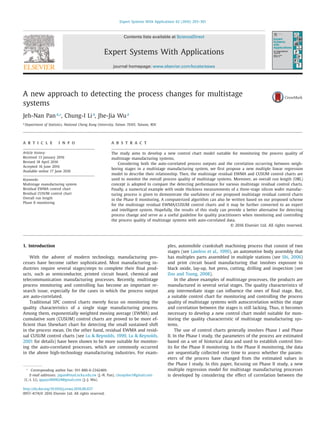
Fig. 1. Structure of a multistage system model.
3.1. The structure of a multistage system model
Let Yi, j be the process variable for jth sample taken from ith
stage. Then, the structure of our proposed multistage system model
can be shown in Fig. 1:
Since AR(1) is a commonly used time series model for autocor-
related data and most researchers such as Lawless et al. (1999),
Agrawal et al. (1999) Yang and Yang (2006), Davoodi and Niaki
(2012) used it to represent the variation transmissions in multi-
stage processes, the 1st stage data can be fitted with the following
AR(1) model:
Y1,j = (1 − φ)ξY1,0
+ φY1,j−1 + ε1,j, j = 1, 2, . . .
where Y1, j is the process variable for jth sample taken from 1st
stage, Y1, j−1 is the process variable for ( j − 1) th sample taken
from the 1st stage, ξY1,0
is the process mean of the 1st stage, φ
is the autoregressive parameter and ɛ1, j is assumed to be an in-
dependent normal random variable with mean 0 and variance σ2
ε1
.
Then, the estimated time series model can be expressed as ˆY1, j =
(1 − ˆφ)ξY1,0
+ ˆφY1, j−1 and the residual of the jth sample taken from
the 1st stage is defined as eY1,j
= Y1, j − ˆY1, j. Starting from the 2nd
stage, the process variable for each stage of a multistage system
can be written as the following multiple regression model without
loss of generality:
⎧
⎪⎪⎪⎪⎪⎨
⎪⎪⎪⎪⎪⎩
Y2,j = β2,0 + β2,1Y2,j−1 + β2,2Y1,j + ε2,j, j = 1, 2, . . .
Y3,j = β3,0 + β3,1Y3,j−1 + β3,2Y2,j + ε3,j, j = 1, 2, . . .
YW−1,j = βW−1,0 + βW−1,1YW−1,j−1 + βW−1,2YW−2,j + εW−1,j,
j = 1, 2, . . .
YW,j = βW,0 + βW,1YW,j−1 + βW,2YW−1,j + εW,j, j = 1, 2, . . .
where Yi, j is the process variable for jth sample taken from ith
stage and Yi, j−1 is the process variable for ( j − 1)th sample taken
from ith stage. βi, 0 is a constant, i = 2, . . . , W. ɛi, j is assumed to be
an independent normal random variable with mean 0 and variance
σ2
εi
, i = 1, . . . , W.
Hence, the least square estimator of process variable for jth
sample taken from ith stage is given by
ˆYi,j = ˆβi,0 + ˆβi,1Yi,j−1 + ˆβi,2Yi−1,j, i = 2, . . . , W
and the residual of jth sample taken from ith stage is defined as
eYi,j
= Yi, j − ˆYi, j, i = 2, . . . , W where eYi,j
is assumed to be an inde-
pendent normal random variable with mean 0 and variance σ2
εi
.
3.2. Multistage residual EWMA control chart
The control statistic for our proposed multistage residual
EWMA control chart is defined as:
Zo = μeYi,j
, j = 0, i = 1, . . .W
Zj = λeYi,j
+ (1 − λ)Zj−1, j = 1, 2, 3 . . . , i = 1, . . . ,W
where eYi,j
is residual of observation from ith stage, λ is smoothing
constant, 0 < λ ≤ 1 and μeYi,j
is initial value. Then, the control
statistic and control limits of residual EWMA control chart can be
written as:
⎧
⎪⎪⎪⎪⎪⎪⎨
⎪⎪⎪⎪⎪⎪⎩
UCL = ZeYi,j
+ LσeYi,j
λ
(2−λ)
1 − (1 − λ)2 j
contorl statistic = ZeYi,j
LCL = ZeYi,j
− LσeYi,j
λ
(2−λ)
1 − (1 − λ)2 j
where L is control limit.
3.3. Multistage residual CUSUM control chart
The control statistic for our proposed multistage residual
CUSUM control chart can be defined as:
CR+
eYi,j
= max 0, eYi,j
− kσei
+ CR+
eYi,j−1
,
CR−
eYi,t
= max 0, −kσei
− eYi,j
+ CR−
eYi,j−1
where eYi,j
is residual of observation from ith stage, kσei
is ref-
erence value, CR+
eYi,0
= CR−
eYi,0
= 0. If the control statistic CR+
eYi,j
or
CR−
eYi,j
exceeds decision limits ±hσei
, then CUSUM control chart will
give the warning signals.
3.4. Criterion for evaluating detecting ability of multistage control
charts
In order to detect the process changes early, the Overall In-
Control Run Length (OIRL) defined in Eq. (1) is proposed as a crite-
rion for evaluating the overall detecting ability of multistage con-
trol charts when a multistage process is in control,
OIRL = min(IRL1, IRL2, IRL3, . . . , IRLi), i ≥ 1 (1)
where IRLi represents the value of in-control run length of ith
stage. When a multistage process is in control, we expect the av-
erage of OIRL ≥ 370 so that type I error rate of overall multistage
system can be maintained at α ≤ 0.27%. Moreover, when a multi-
stage process is out of control, we use the Overall Out-of-Control
Run Length (OORL) defined in Eq. (2) as a criterion for evaluating
the overall detecting ability of multistage control charts, i.e.
OORL = min(ORL1, ORL2, ORL3, . . . , ORLi), i ≥ 1 (2)
where ORLi represents the value of out-of-control run length of ith
stage.
3.4.1. Derivation of cumulative distribution function of overall run
length
Due to the fact that run length follows a geometric distribution
and it is the foundation of the process detection using a control
chart, one can assume that the run length of ith stage also follows
a geometric distribution with success probability αi, denoted by
Geo(αi) and define the overall run length (ORL) as
Y = min(RL1, RL2, . . . , RLW),
where RLi ∼ Geo(αi), i = 1 . . . ,W. The cumulative distribution
function of ORL can be derived as below:
P(Y ≤ y) = P(min(RL1, RL2, . . . , RLW) ≤ y)
= 1 − P(min(RL1, RL2, . . . , RLW) > y)
= 1 − P(RL1 > y, RL2 > y, . . . , RLW > y)
= 1 −
W
i=1
P(RLi > y)
4. 296 J.-N. Pan et al. / Expert Systems With Applications 62 (2016) 293–301
Table 1
Various combinations of control parameters (λ, L) for multistage residual EWMA control
chart in which AOIRLs are close to 370 under different autocorrelations.
AOIRL = 370 (λ, L)
φ = 0.25 (0.05, 2.91) (0.10, 3.11) (0.15, 3.16) (0.20, 3.21) (0.25, 3.24)
φ = 0.50 (0.05, 2.94) (0.10, 3.12) (0.15, 3.17) (0.20, 3.23) (0.25, 3.25)
φ = 0.75 (0.05, 2.98) (0.10, 3.15) (0.15, 3.19) (0.20, 3.25) (0.25, 3.27)
= 1 −
W
i=1
[1 − P(RLi ≤ y)]
= 1 −
W
i=1
1 − 1 − (1 − αi)y
= 1 −
W
i=1
(1 − αi)y
= 1 −
W
i=1
(1 − αi)
y
If we let W
i=1(1 − αi) = 1 − α∗, then P(Y ≤ y) = 1 − (1 − α∗)y,
where α∗ = 1 − W
i=1(1 − αi). It is proven that ORL follows a ge-
ometric distribution with success probability α∗. In practice, if we
assume that type I error rate for each stage are equal, then the
type I error of the overall system can be obtained:
α∗
= 1 − (1 − α)W
Hence, if we set the overall type I error rate is α∗ and divided it
into W stages, then the corrected type I error rate α for each stage
can be obtained as:
α = 1 − (1 − α∗
)
1
W
Similar to the run length, ORL statistics can be extended to
ARMA(p,q) models. Thus, one can use our proposed multistage
residual EWMA and CUSUM control charts to detect the process
change in a multistage manufacturing system if the process data
for each stage follow ARMA(p,q) models.
3.5. Simulation results for multistage residual EWMA control charts
In our simulation studies, once the average of OIRL (AOIRL) is
fixed at 370, the average of OORL (AOORL) is used to evaluate the
detecting performance of multistage residual control charts with
that of Phase II control charts after conducting 1000 simulation
runs. Without loss of generality, we consider a multistage system
with three stages and the sample size is set as 3000 for each stage.
Moreover, the process variances for each stages are assumed to
be homogeneous and the amount of process mean shift for each
stage are also assumed to be the same when a multistage system
is out of control. Based on the same setting of control parameter
as shown in Lucas & Saccucci (1990), the AOIRL of our proposed
multistage residual EWMA control chart using (λ, L) = (0.05, 2.615)
equals 500 when the number of stage is set as W = 1. The AOIRL
of our proposed control chart equals 88.32 when the process mean
shift is set to be δ = 0.25. These two results are fairly closed to
those given by Lucas & Saccucci (1990). Thus, the correctness of
our computer simulation program is confirmed.
By fixing the AOIRL at 370, various combinations of control pa-
rameters for multistage residual EWMA control chart under differ-
ent autocorrelations are listed in Table 1. Table 1 indicates that,
for a given autocorrelation φ, the control limit L increases as the
smoothing constant λ increases; for a given smoothing constant λ,
the control limit L increases slightly as the autocorrelation φ in-
creases.
Table 2
Comparison of AOORLs for multistage residual EWMA control charts
under various combinations of autocorrelations, control parameters and
the process mean shiftsδ.
AOORL δ
(λ, L) 0.25 0.50 0.75 1.00
φ = 0.25 (0.05, 2.91) 56.88 5.40 1.12 1.00
(0.10, 3.11) 96.27 18.98 4.04 1.31
(0.15, 3.16) 118.29 28.82 7.71 2.53
(0.20, 3.21) 146.82 40.22 12.70 4.65
(0.25, 3.24) 165.13 48.66 16.39 6.40
φ = 0.50 (0.03, 2.79) 78.01 8.90 1.31 1.00
(0.05, 2.94) 118.95 25.48 4.88 1.36
(0.10, 3.12) 180.32 54.29 17.69 6.27
(0.15, 3.17) 196.25 69.40 27.00 11.24
(0.20, 3.23) 237.28 89.15 38.16 17.32
(0.25, 3.25) 244.64 103.69 49.30 23.18
φ = 0.75 (0.02, 2.74) 207.11 54.47 12.24 3.09
(0.03, 2.83) 228.25 78.75 29.24 8.65
(0.05, 2.98) 264.71 117.42 52.20 25.25
(0.10,3.15) 327.80 177.95 93.73 53.23
(0.15,3.19) 310.68 191.59 111.03 69.71
(0.20,3.25) 337.12 224.00 139.51 88.98
(0.25,3.27) 335.02 236.75 157.49 103.93
Table 3
Various combinations of control parameters (h, k) for multistage residual CUSUM
control charts in which AOIRLs are close to 370 under different autocorrelations.
AOIRL = 370 (h, k)
φ = 0.25 (15.5, 0.125) (10.1, 0.250) (7.39, 0.375) (5.82, 0.500)
φ = 0.50 (15.5, 0.125) (10.1, 0.250) (7.38, 0.375) (5.84, 0.500)
φ = 0.75 (15.5, 0.125) (10.1, 0.250) (7.41, 0.375) (5.80, 0.500)
As AOORL is used to evaluate and compare the detecting ability
of multistage residual control charts, simulation results of AOORLs
for multistage residual EWMA control charts under various com-
binations of autocorrelations, control parameters and the process
mean shifts are summarized in Table 2. For a given process mean
shift and control parameter, AOORL increases as autocorrelation in-
creases. The comparison results show that the detecting ability of
multistage residual EWMA control chart performs better when the
autocorrelation is small. Thus, it is suggested to choose a smaller
smoothing constant for a process with high autocorrelation. For ex-
ample, λ = 0.03 (λ = 0.02) is a better choice for smoothing con-
stant as the autocorrelation φ = 0.5 (φ = 0.75). In addition, the
optimal choice of smoothing constant is in the range 0.01 < λ ≤
0.05 for a process with moderate or high autocorrelation.
3.6. Simulation results for multistage residual CUSUM control chart
By fixing the AOIRL at 370, various combinations of control pa-
rameters for CUSUM under different autocorrelations (φ = 0.25,
0.5, 0.75) are listed in Table 3. Table 3 indicates that, for a
given autocorrelation, the reference value (k) increases as decision
limit (h) decrease. This result is consistent with the findings of
Hawkins (1993). Moreover, for a given reference value, the decision
limit is insensitive to the autocorrelation.
5. J.-N. Pan et al. / Expert Systems With Applications 62 (2016) 293–301 297
Fig. 2. The Phase II EWMA control charts using control parameter (λ, L) = (0.2, 3.21) if the process mean shift is set as δ = 0.50.
Table 4
Comparison of AOORL s for multistage residual CUSUM control charts
under various combinations of autocorrelations, control parameters and
the process mean shiftsδ.
δ
(h, k) 0.25 0.50 0.75 1.00
φ = 0.25 (15.5, 0.125) 80.67 38.85 25.61 19.24
(10.1, 0.250) 88.75 32.87 19.53 14.02
(7.39, 0.375) 130.47 37.54 17.50 11.85
(5.82, 0.500) 213.83 84.14 17.68 11.04
φ = 0.50 (15.5, 0.125) 126.36 58.20 37.78 28.37
(10.1, 0.250) 146.51 55.82 31.82 22.04
(7.38, 0.375) 192.78 80.85 32.48 19.97
(5.84, 0.500) 261.31 141.37 36.70 20.93
φ = 0.75 (15.5, 0.125) 231.52 122.51 80.28 58.65
(10.1, 0.250) 283.71 151.22 85.24 56.89
(7.41, 0.375) 308.19 201.50 104.42 63.74
(5.80, 0.500) 367.19 293.34 119.54 74.51
Note that the bold figures indicate the reference value k is set as half of
half of process mean shift δ
As AOORL is used to evaluate and compare the detecting abil-
ity of multistage residual control charts, the simulation results of
AOORL s for multistage residual CUSUM control charts under var-
ious combinations of autocorrelations, control parameters and the
process mean shifts are summarized in Table 4. Table 4 indicates
that, for a given process mean shift and control parameter, AOORL
for multistage residual CUSUM control chart increases as the au-
tocorrelation increases. The comparison results show that the de-
tecting ability of multistage residual CUSUM control chart performs
better when the autocorrelation is small.
3.7. Sensitivity analysis
Due to the fact that the number of stages within a multistage
systems increase will cause the type I error of the overall multi-
stage system increases as well. Thus, given the type I error of the
overall multistage system is fixed at 0.27%, a sensitivity analysis
is performed to explore the change in control parameters as the
number of stages increases.
The AOORL values of multistage residual EWMA control chart
under various combinations of autocorrelations, control parame-
ters, the number of stages and the process mean shifts are shown
in Table 5. For a given mean shift and number of stages, the AOORL
value increases as autocorrelation increases. For a given mean shift
and autocorrelation, the AOORL value decreases as the number of
stages increases. Based on the simulation results shown in Table 5,
we can conclude that the detecting ability of proposed multistage
residual EWMA control chart increases as the number of stages in-
creases.
The effects of the number of stages on detecting ability of vari-
ous multistage residual CUSUM control charts are listed in Table 6.
For a given φ, the AOORL value decreases as the number of stages
increases. This means that the detecting ability of multistage resid-
ual CUSUM control chart increases as the number of stage in-
creases.
6. 298 J.-N. Pan et al. / Expert Systems With Applications 62 (2016) 293–301
Fig. 3. The multistage residual EWMA control charts using control parameter (λ, L) = (0.2, 3.21) if the process mean shift is set as δ = 0.50.
Table 5
The AOORL value of multistage residual EWMA control chart under various com-
binations of autocorrelation, control parameters, the number of stage and the pro-
cess mean shift.
AOORL δ
(λ, L) W Stages 0.25 0.50 0.75 1.00
φ = 0.25 (0.10, 3.11) W = 3 96.27 18.98 4.04 1.31
(0.10, 3.25) W = 5 75.38 11.75 2.16 1.08
(0.10, 3.35) W = 7 67.83 9.89 1.85 1.02
φ = 0.50 (0.10, 3.12) W = 3 180.32 54.29 17.69 6.27
(0.10, 3.25) W = 5 144.02 39.73 12.19 4.03
(0.10, 3.35) W = 7 136.27 34.10 9.94 3.04
φ = 0.75 (0.10, 3.15) W = 3 327.80 177.95 93.73 53.23
(0.10, 3.28) W = 5 306.92 152.53 80.64 41.37
(0.10, 3.39) W = 7 304.54 148.44 76.18 38.58
4. Numerical example
To demonstrate the practical application of our proposed
multistage residual control charts, the data set provided by
Montgomery (2008) with thirty (30) oxide thickness measure-
ments taken in the Phase II monitoring of a silicon wafer manu-
facturing process is used for illustration purpose. In this numeri-
cal example, we treat different time frames as different stages (i.e.
Table 6
The AOORL value of multistage residual CUSUM
control chart under various combinations of corre-
lation, control parameters and the number of stage
if the process mean is δ = 1.
AOORL δ
φ (h, k) W Stages 1.00
φ = 0.25 (5.82, 0.50) W = 3 11.04
(6.25, 0.50) W = 5 10.20
(6.65, 0.50) W = 7 9.77
φ = 0.50 (5.84, 0.50) W = 3 20.93
(6.25, 0.50) W = 5 17.65
(6.65, 0.50) W = 7 17.00
φ = 0.75 (5.80, 0.50) W = 3 74.51
(6.25, 0.50) W = 5 61.59
(6.64, 0.50) W = 7 59.87
three different time frames can be viewed as a special case of
three-stage system) and the control limits at different stages are
set as the same in the Phase II monitoring. Moreover, we only use
one point outside control limits as the detecting rule at different
stages and the out-of-control points will be removed from the pro-
cess subsequently. Due to the statistical property of ORL as stated
in Section 3.4.1, our proposed multistage residual EWMA/CUSUM
control charts can be applied to the process change detection of
7. J.-N. Pan et al. / Expert Systems With Applications 62 (2016) 293–301 299
Fig. 4. The Phase II CUSUM using control parameter (h, k) = (5.82, 0.50) when the process mean shift is set as δ = 1.00.
a multistage manufacturing system with the process data for each
stage following ARMA(p, q) models.
4.1. Comparison between Phase Ii EWMA and multistage residual
EWMA control charts
In this example, the Phase II EWMA and multistage residual
EWMA control charts using control parameter (λ, L) = (0.2, 3.21)
are shown in Fig. 2 and Fig. 3 respectively if the process mean
shift is set as δ = 0.50. As one can see from Fig. 2, the Phase II
EWMA control charts cannot detect the mean shift until 3rd stage
and the OORL value is 27. On the other hand, if the process mean
shift is set as δ = 0.50, the multistage residual EWMA control chart
using control parameter (λ, L) = (0.20, 3.21) is able to detect this
mean shift at 1st stage and the OORL value is 6 (see Fig. 3). The
comparison results show that the detecting ability of our proposed
multistage residual EWMA control chart outperforms that of the
Phase II EWMA control chart.
The comparison results of OORLs for the Phase II and multi-
stage residual EWMA control charts under various mean shifts are
summarized in Table 7. Table 7 indicates that, if the process mean
shift is set as δ = 0.25, the Phase II EWMA control chart using con-
trol parameter (λ, L) = (0.10, 3.11) cannot detect this mean. On the
other hand, if the process mean shift is δ = 0.25, the multistage
residual EWMA control chart using control parameter (λ, L) = (0.10,
3.11) is able to detect this mean shift at 1st stage. Moreover, if
the process mean shift is set as δ = 0.25, the multistage residual
EWMA control chart using control parameter (λ, L) = (0.05, 2.91)
Table 7
Comparison between the Phase II EWMA and Multistage Residual EWMA Control
charts under various mean shift (δ).
δ
0.25 0.50 0.75 1.00
Phase II EWMA (λ, L) (0.05, 2.91) 1(I∗
) 1(I∗
) 1(I∗
) 1(I∗
)
(λ, L) (0.10, 3.11) – 1(I∗
) 1(I∗
) 1(I∗
)
(λ, L) (0.15, 3.16) 28(III∗
) 6(II∗
) 1(I∗
) 1(I∗
)
(λ, L) (0.20, 3.21) 28(III∗
) 27(III∗
) 1(I∗
) 1(I∗
)
(λ, L) (0.25, 3.24) 28(III∗
) 27(III∗
) 1(II∗
) 1(I∗
)
Multistage EWMA (λ, L) (0.05, 2.91) 1(I∗
) 1(I∗
) 1(I∗
) 1(I∗
)
(λ, L) (0.10, 3.11) 1(I∗
) 1(I∗
) 1(I∗
) 1(I∗
)
(λ, L) (0.15, 3.16) – 1(I∗
) 1(I∗
) 1(I∗
)
(λ, L) (0.20, 3.21) – 6(I∗
) 1(I∗
) 1(I∗
)
(λ, L) (0.25, 3.24) – 6(I∗
) 1(I∗
) 1(I∗
)
Note: (I∗) indicates that multistage control chart can detect the mean shift at 1st
stage.
and (0.10, 3.11) are able to detect the mean shift at 1st stage. Al-
though the Phase II EWMA control chart using control parameter
(λ, L) = (0.05, 2.91) can detect the mean shift at 1st stage, the
EWMA control chart using control parameter (λ, L) = (0.10, 3.11)
cannot detect the mean shift. Also, it is worth noting that our pro-
posed multistage residual control charts have the advantage of us-
ing cause-selecting charts which preserve the property of diagnos-
ability. Hence, the detecting ability of our proposed EWMA control
charts outperform that of the Phase II EWMA control charts.
8. 300 J.-N. Pan et al. / Expert Systems With Applications 62 (2016) 293–301
Fig. 5. The multistage residual CUSUM control chart using control parameter (h, k) = (5.82, 0.50) if the process mean shift is set as δ = 1.00.
Table 8
Comparison of OORLs between the Phase II CUSUM and Multistage Residual CUSUM Control charts un-
der various mean shifts (δ).
δ
0.25 0.50 0.75 1.00
Phase II
CUSUM (h, k) (15.5, 0.125) (10.1, 0.25) (7.39, 0.375) (5.82, 0.50)
– – 20(II∗
) 8(II∗
)
Multistage CUSUM (h, k) (15.5, 0.125) (10.1, 0.25) (7.39, 0.375) (5.82, 0.50)
– – 9(I∗
) 6(I∗
)
Note: (I∗
) indicates that multistage control chart can detect the mean shift at 1st stage.
4.2. Comparison between Phase II CUSUM and multistage residual
CUSUM control charts
The Phase II CUSUM control charts using control parameter (h,
k) = (5.82, 0.50) are shown as in Fig. 4 when the process mean
shift is set as δ = 1.00. As shown in Fig. 4, the Phase II CUSUM
control chart cannot detect the mean shift until 2nd stage. The
OORL value is 8.
If the process mean shift is set as δ = 1.00, the multistage
residual CUSUM control chart using the same control parameter is
shown in Fig. 5. Note that the multistage residual CUSUM control
chart will be able to detect this mean shift at 1st stage and the
OORL value is 6.
In addition, the comparison results of OORLs for the Phase II
and multistage residual CUSUM control charts under various pro-
cess mean shifts are summarized in Table 8. Note that, if the pro-
cess mean shift is set as δ = 0.75, the multistage residual CUSUM
control chart is able to detect the mean shift at 1st stage (OORL
= 9), whereas the Phase II CUSUM control chart cannot detect the
mean shift until 2nd stage (OORL = 20). Based on the compar-
ison results shown in Tables 7 and 8, we can conclude that the
detecting ability of our proposed multistage residual EWMA and
CUSUM control charts outperform that of the Phase II EWMA and
CUSUM control charts. Moreover, our proposed multistage residual
control charts have the advantage of using cause-selecting charts
which preserve the property of diagonosibility. Hence, the detect-
ing ability of our proposed control charts outperform that of the
Phase II control charts.
5. Conclusions and discussions
Considering both the autocorrelated process outputs and the
correlation occurring between neighboring stages, we have suc-
cessfully developed a new multiple regression model for mul-
9. J.-N. Pan et al. / Expert Systems With Applications 62 (2016) 293–301 301
tistage manufacturing systems. Then, the residual EWMA and
CUSUM control charts for each stage are constructed accordingly.
An Overall Run Length (ORL) concept is adopted as the criterion
for evaluating the detecting ability of multistage control charts.
The simulation results show that the detecting ability performs
better when the autocorrelation is smaller for multistage resid-
ual EWMA and CUSUM control charts. The cumulative distribution
function (CDF) of ORL is further derived to confirm the correct-
ness of ORL. Finally, a numerical example further illustrates that
the detecting ability of our proposed multistage residual EWMA
and CUSUM control charts outperform that of the existing Phase II
EWMA and CUSUM control charts respectively. Both simulation re-
sults and numerical example indicate that our proposed approach
provide more precise process control for auto-correlated process
outputs. It is worthy to note that, in our simulation study, the pro-
cess variances for each stage is assumed to be homogeneous and
the amount of process mean shifts for each stage are assumed to
be the same when a multistage system is out of control. These as-
sumptions may be lifted in the future studies. Again, the process
data for each stage are assumed to be stationary and follow AR(1)
model without loss generality. Future studies may consider the
cases for other time series models as well as profile data. Similar
research can be extended to develop multivariate residual MEWMA
and MCUSUM control charts for multistage manufacturing systems
with multiple quality characteristics.
Moreover, our proposed multistage EWMA and CUSUM residual
control charts can be further extended to the quality surveillance
of other multistage systems as they have the advantage of using
cause-selecting charts which preserve the property of diagonosi-
bility. In contrast with the quality surveillance using the existing
Phase II control charts, one can effectively distinguish a special
cause occurs in a particular stage and thus provides diagnostic in-
formation regarding which stage is out-of-control using our pro-
posed scheme. Although the assumption of our proposed multi-
stage residual EWMA and CUSUM control charts is based on the
AR(1) model, it can be extended to other time series models, such
as ARMA(p, q),etc. Thus, the new approach provides a better al-
ternative for detecting the process change in multistage systems
with auto-correlated process outputs. A computerized algorithm
can also be written based on our proposed scheme for the mul-
tistage residual EWMA/CUSUM control charts and it may be fur-
ther converted to an expert and intelligent system. Hopefully, the
results of this study can provide a better alternative for detecting
process change and serve as a useful guideline for quality prac-
titioners when monitoring and controlling the process quality for
multistage systems with auto-correlated data in the Phase II mon-
itoring.
Acknowledgement
The first author would like to gratefully acknowledge financial
support (MOST 104-2410-H-006-049) from the Ministry of Science
and Technology of Taiwan, ROC.
References
Asadzadeh, S., & Aghaie, A. (2012). Improving the product reliability in multistage
manufacturing and service operations. Quality and Reliability Engineering Inter-
national, 28(4), 397–407.
Asadzadeh, S., Aghaie, A., & Shahriari, H. (2013). Cause-selecting charts based on
proportional hazards and binary frailty models. International Journal of Industrial
Engineering and Production Research, 24(2), 107–112.
Asadzadeh, S., Aghaie, A., Shahriari, H., & Niaki, S. T. A. (2015). Improving reliability
in multistage processes with autocorrelated observations. Quality Technology and
Quantitative Management, 12(2), 143–157.
Davoodi, M., & Niaki, S. T. A. (2012). Estimating the step-change time of the location
parameter in multistage processes using MLE. Quality and Reliability Engineering
International, 28, 843–855.
Hawkins, D. M. (1991). Multivariate quality control based on regression -adjusted
variables. Technometrics, 33(1), 61–75.
Hawkins, D. M. (1993). Cumulative sum control charting: An underutilized SPC tool.
Quality Engineering, 5(3), 463–477.
Lawless, L. F., MacKay, R. J., & Robinson, J. A. (1999). Analysis of variation trans-
mission in manufacturing processes-part I. Journal of Quality Technology, 31(2),
131–142.
Lu, C. W., & Reynolds, M. R. (1999). EWMA control charts for monitoring the mean
of autocorrelated processes. Journal of Quality Technology, 31(2), 166–188.
Lu, C. W., & Reynolds, M. R. (2001). CUSUM charts for monitoring an autocorrelated
processes. Journal of Quality Technology, 33(3), 66–81.
Lucas, J. M., & Saccucci, M. S. (1990). Exponentially weighted moving average control
schemes: properties and enhancements. Technometrics, 32(1), 1–29.
Montgomery, D. C. (2008). Introduction to statistical quality control (p. 278). New
York: John Wiley & Sons.
Shi, J. (2006). Stream of variation modeling and analysis for multistage manufacturing
processes. Boca Raton, FL: CRC Press.
Tsung, F, & Xiang, L (2004). Multistage process control and monitoring via group
EWMA schemes. Institute of Electrical and Electronic Engineers, 2, 1087–1092.
Yang, S. F., & Yang, C. M. (2006). An approach to controlling two dependent process
steps with autocorrelated observations. International Journal of Advanced Manu-
facturing Technology, 29(1), 170–177.
Yang, S. F., Lin, J. S., & Cheng, S. W. (2011). A new nonparametric EWMA sign control
chart. Expert Systems with Applications, 38(5), 6239–6243.
Zhang, G. X. (1984). A new type of control charts and a theory of diagnosis with
control charts. In World quality congress transactions (pp. 175–185). London:
American Society for Quality Control.
Zhang, G. X. (1987). Cause-selecting control charts a new type of quality control
charts. 41st Annual Quality Congress, Minneapolis, MN, 41(0), 16–21.
Zhang, G. X. (1990). A new diagnosis theory with two kinds of quality. Total Quality
Management, 1(2), 249–257.
Zhang, G. X. (1992). Cause-selecting control chart and diagnosis, theory and prac-
tice. Department of total quality management. Aarhus School of Business. Aarhus,
Denmark.
Zou, C., & Tsung, F. (2008). Directional MEWMA schemes for multistage process
monitoring and diagnosis. Journal of Quality Technology, 40(4), 407–427.