IOSR Journal of Mathematics(IOSR-JM) is a double blind peer reviewed International Journal that provides rapid publication (within a month) of articles in all areas of mathemetics and its applications. The journal welcomes publications of high quality papers on theoretical developments and practical applications in mathematics. Original research papers, state-of-the-art reviews, and high quality technical notes are invited for publications.

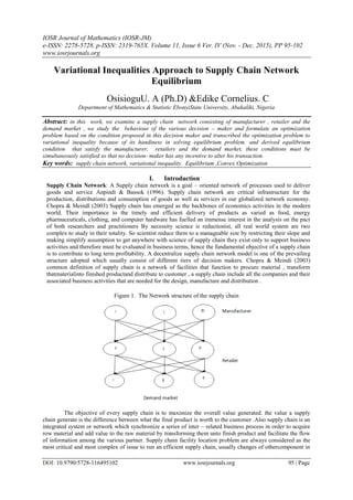
1. IOSR Journal of Mathematics (IOSR-JM)
e-ISSN: 2278-5728, p-ISSN: 2319-765X. Volume 11, Issue 6 Ver. IV (Nov. - Dec. 2015), PP 95-102
www.iosrjournals.org
DOI: 10.9790/5728-116495102 www.iosrjournals.org 95 | Page
Variational Inequalities Approach to Supply Chain Network
Equilibrium
OsisioguU. A (Ph.D) &Edike Cornelius. C
Department of Mathematics & Statistic EbonyiState University, Abakaliki, Nigeria
Abstract: in this work, we examine a supply chain network consisting of manufacturer , retailer and the
demand market , we study the behaviour of the various decision – maker and formulate an optimization
problem based on the condition proposed in this decision maker and transcribed the optimization problem to
variational inequality because of its handiness in solving equilibrium problem. and derived equilibrium
condition that satisfy the manufacturer, retailers and the demand market, these conditions must be
simultaneously satisfied so that no decision- maker has any incentive to alter his transaction.
Key words: supply chain network, variational inequality. Equilibrium ,Convex Optimization
I. Introduction
Supply Chain Network: A Supply chain network is a goal – oriented network of processes used to deliver
goods and service Anpindi & Bassok (1996). Supply chain network are critical infrastructure for the
production, distributions and consumption of goods as well as services in our globalized network economy.
Chopra & Meindl (2003) Supply chain has emerged as the backbones of economics activities in the modern
world. Their importance to the timely and efficient delivery of products as varied as food, energy
pharmaceuticals, clothing, and computer hardware has fuelled an immense interest in the analysis on the pact
of both researchers and practitioners By necessity science is reductionist, all real world system are two
complex to study in their totality. So scientist reduce them to a manageable size by restricting their slope and
making simplify assumption to get anywhere with science of supply chain they exist only to support business
activities and therefore must be evaluated in business terms, hence the fundamental objective of a supply chain
is to contribute to long term profitability. A decentralize supply chain network model is one of the prevailing
structure adopted which usually consist of different tiers of decision makers. Chopra & Meindi (2003)
common definition of supply chain is a network of facilities that function to procure material , transform
thatmaterialinto finished productand distribute to customer , a supply chain include all the companies and their
associated business activities that are needed for the design, manufacture and distribution .
Figure 1. The Network structure of the supply chain
The objective of every supply chain is to maximize the overall value generated. the value a supply
chain generate is the difference between what the final product is worth to the customer .Also supply chain is an
integrated system or network which synchronize a series of inter – related business process in order to acquire
row material and add value to the raw material by transforming them unto finish product and facilitate the flow
of information among the various partner. Supply chain facility location problem are always considered as the
most critical and most complex of issue to run an efficient supply chain, usually changes of othercomponent in

2. Variational Inequalities Approach To Supply Chain Network Equilibrium
DOI: 10.9790/5728-116495102 www.iosrjournals.org 96 | Page
supply chain such as transportation and information system can be made with less hassle due to relatively bigger
amount of choice. In other words.These types of decision can be readily re- optimized in response to changes.
A common definition of supply chain is a network of facilities that function to procure material , transform that
material into finished product and distribute to customer , a supply chain include all the companies and their
associated business activities that are needed for the design, manufacture and distribution .
Many classical economics equilibrium problems have been formulated as a system of equation, since
market clearing conditions necessary equate the total supply with the total demand In terms of a variation
inequality problem This chapter discusses the definition and analysis aspect that are necessary for a
conceptualization of general applicability for supply chain network, and approach behind concept of optimality
condition of manufacturer, retailer and consumer. Variational inequality formulation as a facilitator to supply
chain network equilibrium.
II. Introduction Of Equilibrium Model.
In the classical circumstance we address there are agent called consumer, index by 𝑘 = 1 … … 𝑜 along
with agent called producer index by = 1 … … . 𝑚 . both deal with goods indexed by 𝑗 = 1 … … . . 𝑛 , vector 𝑅 𝑘;
having component that stand for quantities of these goods will be involved in both consumption and production
for each consumer 𝑘 there is a consumption set 𝑋𝑖 𝑐 R
𝑘
, whereas for each producer 𝑖 there is a production set
𝑌𝑖 𝐶 R
𝑘
consumer 𝑘 will chose a consumption vector 𝑥𝑖 𝜖𝑋 𝑘 and producer 𝑖 will chose a production vector
𝑦𝑖 𝜖𝑌𝑗 . consumption vector 𝑥𝑖 are related by agent 𝑖 according to their utility, which is described by a function
𝑢𝑖 𝑜𝑛𝑋𝑖 ; the higher the utility value 𝑢𝑖(𝑥𝑖) the better. Obviously the chosen 𝑥𝑖 𝑠𝑎𝑛𝑑𝑦𝑖 𝑠 must turn out to be such
that the total consumption 𝑥1
𝑖=1 i does not exceed the total (net) production 𝑦
𝑗
𝑖=1 j plus the total endowment
𝑒1
𝑖=1 i. The coordination is to be achieved by a market in which goods can be traded at particular prices. The
prices are not part of the given data, hence they must be determined from interaction of the consumer, retailer
and producer over availabilities and preference .this is why finding equilibrium is much more than just a matter
of optimization. In this study we developed a fixed demand version of the supply chain network model , the
model consist of 𝑚 manufacturer ,𝑛 retailer 𝑜 demand market in figure (1) we denote a typical manufacturer by
𝑖 and typical retailer by 𝑗 and typical demand market by 𝑘 .The links in the supply chain network represent
transportation links. The equilibrium solution is denoted by (∗) all vector are assumed to be column vector.
Therefore we first show the behaviour of the manufacturer and retailers, were then discus the behaviour of the
consumer at the demand market. Finally we state the equilibrium condition for the supply chain network
The fundamental problem of optimization is to arrive at the best possible decision in any given set of
circumstance. In real life problem situation may arise where the best is unattained .the first step in mathematical
optimization is to set up a function whose variable are the variable interest. The function could be linear or non-
linear. This function is better maximized or minimized subject to one or more constrained equation.
This is optimization problem in standard form.
Min/Max 𝑓 𝑥 … … … … … … …....................... equation (1)
s.t 𝑓𝑖 𝑥 ≤ 0 𝑖 = 1 … … … . . 𝑚
𝑓𝑖 𝑥 = 0 𝑖 = 1 … … … . . 𝑝
Therefore 𝑥 ∈ R
𝑛
is the optimization variable
𝑓0 : 𝑅 𝑛
→ R is the objective or cost function.
𝑓𝑖 ∶ R
𝑛
→ R ; 𝑖 = 1 … … 𝑚are the inequality constraint
ℎ𝑖: R
𝑛
→ R are the equality constraint.
An optimization problem is characterized by its given specific objective function that is maximize or
minimized given set of constraint possible objective function include expression representing profit cost ,
market share , both constrained and unconstrained problem can be formulated as variational inequality problem
the subsequent two preposition and theorem identify the relationship between an optimization problem and
variational inequality problem.
The next theorem provides the basis of the relationship that exist between optimization problem and
variational inequality problem.
Theorem 1
Let 𝑥∗
be a solution to the optimization problem
Min𝑓 𝑥 … … … … … … … … … … … … … … . . (4)
s.t𝑥 ∈ 𝐾
Where 𝑓is continuously differentiable and 𝑘 is close and convex , then 𝑥∗
is a solution of the
variational inequality problem

3. Variational Inequalities Approach To Supply Chain Network Equilibrium
DOI: 10.9790/5728-116495102 www.iosrjournals.org 97 | Page
∇𝑓 𝑥∗
, 𝑥 − 𝑥∗
≥ 0∀𝑥 ∈ 𝐾 … … … … … . ( 5)
Proof.
Let ∅ 𝑡 = 𝑓(𝑥∗
+ 𝑡 𝑥 − 𝑥∗
) 𝑓𝑜𝑟𝑡𝜀 0 1
Since ∅ 𝑡 achieve its minimum at 𝑡 = 0
0 ≤ ∅!
0 = ∇𝑓 𝑥∗
. 𝑥 − 𝑥∗
𝑖𝑒
𝑥∗
Is a solution of∇𝑓 𝑥∗
𝑇. 𝑥 − 𝑥∗
≥ 0
Theorem 2
If 𝑓(𝑥) is a convex function and 𝑥∗
is a solution to 𝑉𝐼(∇𝑓, 𝑘) then 𝑥∗
is a solution to the optimization problem
Min 𝑓 𝑥 … … … … … … … … … … … … … … … … … 6
s.t𝑥𝜖𝐾
Proof: since 𝑓 𝑥 is convex
𝑓 𝑥 ≥ 𝑓 𝑥∗
+ ∇𝑓 𝑥∗
. 𝑥 − 𝑥∗
∀𝑥𝜖𝑘 … … … … … … … ( 7)
But ∇𝑓 𝑥∗ 𝑇
. 𝑥 − 𝑥∗
≥ 0
Since 𝑥∗
is solution to 𝑉𝐼(∇𝑓, 𝑘)
Therefore from (6) we conclude that 𝑓 𝑥 ≥ 𝑓 𝑥∗
∀𝑥𝜖𝑘
Variational inequality theory : ( Variational Inequality). The finite – dimensional variational inequality
problem 𝑉𝐼 (𝑓, 𝑘) is to determine a vector 𝑥∗
𝜖𝑘𝑐 R
𝑁
such that
𝑓 𝑋∗
, 𝑋 − 𝑋∗
≥ 0 ∀𝑥𝜖𝐾 … … … … … … … … … … … … … … ..(8)
Where 𝑓 is a given continuous function from 𝐾𝑡𝑜𝑅 𝑁
K is a given closed convex set and . . denote
the inner product in R Or equivalently 𝐹 𝑥∗
𝑇, (𝑥 − 𝑥∗
≥ 0 ∀𝑥𝜖𝑘 where 𝑓 is a given continuous function
from 𝐾 is close and convex set and . . denote the inner product in 𝑛 − 𝑑𝑖𝑚𝑒𝑛𝑠𝑖𝑜𝑛𝑎𝑙𝑠𝑝𝑎𝑐𝑒. Variational
inequality are closely related with many general non linear analysis. Such as complementarity, fixed point and
optimization problem. The simplest example is variational inequality is the problem of solving a system of
equation, the variational inequality is the problem of finding a point 𝑢∗
𝜖𝐾 such that. 𝐺 𝑢∗
, 𝑢 − 𝑢∗
≥
0 ∀𝑢𝜖𝐾 … … … . ( 9)
2.1 The Manufacturer Behaviour And Optimality Condition
Let 𝑝1𝑖𝑗
∗
denote the price charge for the product by manufacturer 𝑖 in transacting with retailer 𝑗 the price
𝑃1𝑖𝑗
∗
is an endogenous variable and will be determined once the entire supply chain network equilibrium model
is solved .we assume that the quantity produce by manufacturer 𝑖 must satisfy the following conservation of
flow of equation
1
n
i ij
j
q q

  .................................................( 15)
Which state that the quantity of product produced by manufacturer 𝑖 is exactly equal to the sum of
quantities transacted between a manufacturer and the retailer, the production cost function 𝑓𝑖 for each
manufacturer 𝑖 ; 𝑖 … … … . 𝑚 be expresses as a function of the flows? 𝑄1
, Assuming that the manufacturer are
profit maximize, we can express the optimization problem as
* 1
1 1
max ( ) ( )
n n
ij ij i ij ij
j j
p q f Q c q
 
  
. : 0ijs t q  for all ; 1,.....j j n
the first term in equation (16) represent price charge , and subsequent terms the product cost and
transaction cost for each manufacturer are continuously differentiable and convex , the optimality condition for
all manufacturer 𝑖 can be expressed as the following variational inequality determine 𝑄1
𝜖𝑅+
𝑚𝑛
𝑠𝑎𝑡𝑖𝑠𝑓𝑦
*1*
* * 1
1
1 1
( )( )
0 .....(17)
m n
ij ij mni
ij ij ij
i j ij ij
c qf Q
p q q Q R
q q

 
 
             

2.2 Retailer Behaviour And Their Optimality Condition.
The retailers in turn purchase the product from the manufacturer and transact with the customer at the
demand market. Thus a retailer is involved in transacting both with the manufacturer as well as with the demand

4. Variational Inequalities Approach To Supply Chain Network Equilibrium
DOI: 10.9790/5728-116495102 www.iosrjournals.org 98 | Page
market. Let 𝑝2𝑗
∗
denote the price charge by he retailer 𝑗 ,for the product. This price will be determined
endogenously after the model is solved. We assume also that the retailer are profit maximize, hence the
optimization problem faced by a retailer 𝑗is given by
max 𝑝2𝑗
∗
𝑛
𝑘=0
𝑞𝑗𝑘 − 𝑐𝑗 𝑄1
− 𝑝1𝑖𝑗
∗
𝑚
𝑖=1
𝑞𝑖𝑗 … … … … … … (18)
𝑠. 𝑡 𝑞𝑗𝑘
0
𝑘=1
≤ 𝑞𝑖𝑗
𝑚
𝑖=1
… … … … … … . . . (19)
Where𝑞𝑖𝑗 ≥ 0 𝑎𝑛𝑑𝑞𝑗𝑘 ≥ 0 𝑓𝑜𝑟𝑎𝑙𝑙𝑖 ; 𝑖 = 1 … . . 𝑚𝑎𝑛𝑑𝑘 ; 𝑘 = 1 … 0 the first term in (18) represent
price charge and the second and third term represent handling cost and payout cost to the manufacturer . hence
constrain (19) expresses that total quantity of the product transacted with the demand market by a retailer
cannot exceed the amount that the retailer has obtained from the manufacturer. Also handling cost for each
retailer is continuously differentiable and convex. Then the optimality condition for all the retailer can be
expressed as the following variation inequality
Determine
1* 2* *
( , , ) mn no n
Q Q R satisfying  

1*
* * * * *
1 2
1 1 1 1
* * * 1 2
1 1 1
( )
0 ( , , ) ..........(20)
m n n o
j
ij ij ij j j jk jk
i j j kij
n m o
mn no n
ij jk j j
j i k
c Q
p q q p q q
q
q q Q Q R

  
   
 

  
 
                        
 
         
 
 
  
The term 𝛾𝑗 is the Lagrange multiplier or shadow price associated with constraint (19) for retailer 𝑗 and  is
the n – dimensional vector of all the shadow prices.
2.3 The Consumer Demand Market And Equilibrium Condition.
The consumer take account the price charged by the retailer and the unit transaction cost incurred to
obtain the product in making their consumption decision, we assume dynamic model in which we allow the
demand to be time varying. The following conservation of flow equation must hold
,
1
1, .......
n
k jk
j
d q k o

 
Where 𝑑 𝑘 is fixed for each demand market K. We assume the unit transaction cost function 𝑐𝑗𝑘 are
continuous function for 𝑗 ; 𝑗 = 1 … . . 𝑛𝑎𝑛𝑑𝑘; 𝑘 = 1 … . .0
The equilibrium condition for consumer at the demand market 𝑘 then take the form for each retailer 𝑗 ; 𝑗 =
1 … … . . 𝑛
𝑝2𝑗
∗
+ 𝑐𝑗𝑘 𝑄2∗
= 𝑝3𝑘 ,𝑖𝑓 𝑞 𝑗𝑘
∗
≥0
∗
≥ 𝑝3𝑘𝑖𝑓 𝑞 𝑗𝑘
∗
= 0
∗ … … … … … . (22)
Equation (22) state that in equilibrium, if the consumer at demand market 𝑘 purchase the product from
retailer 𝑗 then the price the consumer pay is exactly equal to the price charge by retailer plus the unit transaction
cost .however if the sum of the prince charge by the retailer and the unit transaction cost exceed the price that
the consumer is willing to pay at the demand market, there will be no transaction. In equilibrium condition (22)
must hold simultaneously for all demand market, we express the equilibrium condition as the variation
inequality determine 𝑄2∗
𝜀𝑘1
such that
* 2* *
2
1 1
( ) 0
n o
j jk jk jk
j k
p c Q q q
 
         
2 1
,Q K 
Where
1 2
(21) ............(23)no
K Q R and hold 
In equilibrium the optimality condition of the entire manufacturer, the optimality condition for all the
retailers and the equilibrium condition for all the demand market must be simultaneously satisfied so that no
decision maker has any incentive to alter his transaction.

5. Variational Inequalities Approach To Supply Chain Network Equilibrium
DOI: 10.9790/5728-116495102 www.iosrjournals.org 99 | Page
Definition (3) Supply Chain Network Equilibrium.
The equilibrium state of the supply chain network is one where the product flows between the tiers of
network coincide and the product flows satisfy the conservation of flow equation of the sum of optimality
condition of manufacturer, the retailer and the equilibrium condition at the demand markets.
3.4 Variational Inequality Formulation Of Supply Chain Network Equilibrium:The equilibrium condition
governing the supply chain network according to definition 3 coincide with the solution of the (finite –
dimensional) Variational inequality given by:
determine,
1* 2* * 2
( , , )Q Q K satisfying 
* 1*1*
* *
1 1
( ) ( )( )m n
ij ij ji
j ij ij
i j ij ij ij
c q c Qf Q
q q
q q q

  
  
            

2* * * * * *
1 1 1 1 1
( ) 0
n o n m o
jk j jk jk ij jk j j
j k j i k
c Q q q q q  
    
 
                   
 
   
1 2 2
( , , )Q Q K  Where
 2 1 2
, , (21) ........(24)mn no n
K Q Q R and holds  
 
Proof : We first demonstrate that an equilibrium pattern according to definition (3) satisfies the variational
equality, summing up inequalities 17, 20 and 23, after algebraic simplication we obtain (24). We now show the
converse, that is a solution to Variation inequality (24) satisfies the sum of condition 17, 20, & 23 and is
therefore a supply chain network equilibrium pattern first we add the term−𝑝1𝑖𝑗
∗
+ 𝑝1𝑖𝑗
∗
to the first term in the
first summed expression in (24), then, we add the term −𝑝2𝑗 +
∗
𝑝2𝑗
∗
to the first term in the second summed
expression in (24) because these term are all equal to zero , they do not change(24) we obtain the following
inequality
* 1*1*
* * * *
1 1
1 1
( ) ( )( )m n
ij ij ji
j ij ij ij ij
i j ij ij ij
c q c Qf Q
p p q q
q q q

 
  
              

2* * * * *
2 2
1 1
( )
n o
jk j j j jk jk
j k
c Q p p q q
 
           
* * * 1 2 2
1 1 1
0 ( , , ) ........(25)
n m o
ij jk j j
j i k
q q Q Q K  
  
 
          
 
  
Which can be rewritten as?
*1*
* *
1
1 1
( )( )m n
ij iji
ij ij ij
i i ij ij
c qf Q
p X q q
q q 
 
         
 +
1*
* * *
1
1 1
( )m n
j
ij j ij ij
i j ij
c Q
p X q q
q

 
 
        
 +
* * *
2
1 1
n o
ij j jk jk
j k
p X q q
 
         +
 * * 2* *
2
1 1 1 1 1
( )
n m o n o
ij jk jk jk jkj
j i k j k
q q p c Q X q q
    
 
       
 
    0
1 2 2
( , , ) ....................(26)Q Q K 

6. Variational Inequalities Approach To Supply Chain Network Equilibrium
DOI: 10.9790/5728-116495102 www.iosrjournals.org 100 | Page
Clearly (26) is equal to the sum of the optimality conditions of manufacturer, retailer and the consumer
demand market (23) and is, hence variational inequality governing the supply chain network equilibrium in
definition (3) Hence the Variational inequality problem of (24) can be written in standard variational inequality
form as follows: determine 𝑋∗
𝜖𝑘 satisfying
* *
( ), 0 ..............(27)f x x x x K    where𝑋 ≡ (𝑄1
, 𝑄2
, 𝛾, ) and
𝑓 𝑥 ≡ 𝑓𝑖𝑗 , 𝑓𝑗𝑘 , 𝑓𝑗, 𝑓𝑘 𝑖 = 1 … . . 𝑚; 𝑗 = 1 … . . 𝑛; 𝑘 = 1 … 𝑜.
3.41 Corrolary
This corollary established that in equilibrium, the supply chain with fixed demand, since we are
interested in the market clearing ,the market for the product clears for each retailer in the supply chain network
equilibrium that is
𝑞𝑖𝑗
∗
= 𝑞𝑗𝑘
∗
𝑓𝑜𝑟𝑗 = 1 … … . 𝑛
𝑛
𝑗 =1
𝑚
𝑖=1
Clearly from equation (19) if 𝛾𝑗
∗
> 0 𝑡ℎ𝑒𝑛
* *
1 1
m o
jkij
i k
q q
 
  h𝑜𝑙𝑑𝑠 now we consider the
case where 𝛾𝑗
∗
= 0 for some retailer j we examine the first term in inequality (19) since we assume that the
production cost function , the transaction cost function and the handling cost function are convex , it is therefore
to assume that either the marginal production cost or the marginal transaction cost or the marginal handling cost
for each manufacturer /retailer is strictly positive at equilibrium.
Then
* 1*1*
( ) ( )( ) ij ij ji
ij ij ij
c q c Qf Q
q q q
 
 
  
> 0
Which implies that 𝑞𝑖𝑗
∗
= 0 𝑓𝑜𝑟𝑎𝑙𝑙𝑖𝑓𝑜𝑟𝑡ℎ𝑎𝑡𝑗, it follows then from the third term in (19) that
0
*
1
0jk
k
q

 Hence we have that
0
* *
1 1
0
m
jk ij
k i
q q
 
   . for any j such that
*
0j 
there we conclude that the market clears for retailer in the supply chain equilibrium, the price that exist when a
market is in equilibrium, the equilibrium price equate the quantity demanded and quantity supply, more over the
equilibrium price is simultaneously equal to both the demand price and supply price, the equilibrium price is
also commonly referred to as the market clearing price. Since we are interested in the determination of
equilibrium flow and price, we transform constrain (19) into
1 1
.................(28)
o m
jk ij
k i
q q
 
 
Now we can define the feasible set as
3 1 1
( , ) mn no
K Q Q R 
  such that (27) holds
For notational convenience we let ,
1
1,.......
o
j jk
k
S q j n

 
Note that, special case of demand function and supply function that are separable, the jacobians of
these function are symmetric since they are diagonal and given, respectively by
∇𝑠 𝑝 =
𝜕𝑠1
𝑑𝑝1
0 0 0
0
𝜕𝑠2
𝑑𝑝2
0 0
0 0 0
𝜕𝑠𝑛
𝑑𝑝 𝑛

7. Variational Inequalities Approach To Supply Chain Network Equilibrium
DOI: 10.9790/5728-116495102 www.iosrjournals.org 101 | Page
∇d 𝑝 =
𝜕𝑑1
𝑑𝑝1
0 0 0
0
𝜕𝑑2
𝑑𝑝2
0 0
0 0 0
𝜕𝑑 𝑛
𝑑𝑝 𝑛
In this special case model the supply of a product or commodity depends only upon the price of that
commodity while the demand for a commodity depends only upon the price of that commodity. Hence the price
vector 𝑝∗
that satisfies the equilibrium condition can be obtained by solving the following optimization problem
𝑚𝑎𝑥/𝑚𝑖𝑛 𝑆𝑖 𝑥 𝑑𝑥 − 𝑑𝑖 𝑦 𝑑𝑦
𝑝 𝑖
0
𝑛
𝑖=1
𝑝 𝑖
0
𝑛
𝑖=1 ......................(34)
𝑠𝑢𝑏𝑗𝑒𝑐𝑡𝑡𝑜𝑝𝑖 ≥ 0 , 𝑖 = 1 … … . 𝑛
Hence the quantity of product demanded from demand market is equal to the quantity of product
supply.
Example 1, We consider a network structure consist of single manufacturer, a single Retailer and Single demand
market as show below
The manufacturer production cost function is given by 𝑓𝑖 𝑞 = 𝑞1
2
+ 5𝑞1
The transaction cost between the manufacturer and retailer pair is 𝑐11(𝑞11)=𝑞11
2
+ 2𝑞11
The handling cost at the Retailer is 𝑐1 𝑄1
= 2(𝑞11)2
and the unit transaction cost associated with the
transaction between the retailer and demand market is 𝑐11 𝑄1
= 𝑞11 + 1 with the demand function given by
𝑑1 𝑝3 = −𝑝31 + 100 view of these function , the corollary which show that the equilibrium product flow
between the manufacturer and the retailer is equal to the equilibrium product between the retailer and the
demand market , therefore Variational inequality (24) of this example takes the form determine (𝑞11,
∗
𝛾1,
∗
𝜌31
∗
)
(all the value being nonnegative) and satisfying
2 𝑞11
∗
+ 5 + 2𝑞11
∗
+ 2 + 4𝑞11
∗
− 𝑞11
∗
× 𝑞11 − 𝑞11
∗
+ 𝑞11
∗
+ 1 + 𝛾1
∗
− 𝑝31
∗
× 𝑞11 − 𝑞11
∗
+ 𝑞11
∗
− 𝑞11
∗
×
𝛾1 − 𝛾1
∗
+ 𝑞11
∗
+ 𝜌31
∗
− 100 × 𝜌31 − 𝜌31
∗
≥ 0 ∀𝑞11 ≥ 0 ∀𝛾1 ≥ 0 ∀𝜌31 ≥ 0
Combining the like terms in this inequality, after algebraic simplication yields
9 𝑞11
∗
+ 8 − 𝑝31
∗
𝑞11 − 𝑞11
∗
+ 𝑞11
∗
+ 𝑝31
∗
− 100 × 𝑝31 − 𝑝31
∗
≥ 0
Now if we let 𝑞11 = 𝑞11
∗
, we assume that the equilibrium demand market price 𝑝31
∗
is positive , then
substituting into the inequality above gives
𝑝31
∗
= 1 00 − 𝑞11
∗
Therefore letting 𝑝31 = 𝑝31
∗
, substituting now into the same inequality, with𝑝31
∗
= 100 − 𝑞11
∗
gives us 9𝑞11
∗
+ 8 − 100 + 𝑞11
∗
× 𝑞11 − 𝑞11
∗
≥ 0 Assuming that the product flow 𝑞11
∗
is positive ( so that the
manufacturer produces the product) we can conclude that 10𝑞11
∗
− 92 = 0 hence 𝑞11
∗
= 9.20
Then the demand market price is 𝑝31
∗
= 90.80 , the shadow price 𝛾1
∗
can be determined from the above
variational inequality , we obtain 𝛾1=
∗
80.60
III. Conclusion:
In conclusion this seminar work has succeeded in clarifying the use of variational inequality as a tool
in supply chain network for finding the optimality conditions for these three tiers of decision- maker and their
equilibrium condition. Such that each must be simultaneously satisfied so that no decision- maker has any
incentive to alter his transaction and provides a market clearing condition.

8. Variational Inequalities Approach To Supply Chain Network Equilibrium
DOI: 10.9790/5728-116495102 www.iosrjournals.org 102 | Page
References
[1]. Fisher M.L. What is the Right supply chain for your product? Harvard Business Review 75 (2 march – April) 105- 116 (1997).
[2]. Lee H. L and Belington C. The evolution of supply chain management models and practice at Hewlett – Packard interface (1995)
[3]. D. Kinderlehrerand G.Stampachia (1980) . An introduction to Variational Inequalities and their application, Academic press, New
York.
[4]. R .Anupindi and Y ,bassok (1996) Distribution channel ,information system and virtual centralized proceedings of the
manufacturing and services operation management of society conference 87-92.
[5]. Chopra. S Meindl P. (2003) . Supply chain management strategy, planning and operation 2nd
ed Prentice Hall.
[6]. Simchi – Levi, D , Designing and managing the supply chain concepts, strategies and case studies . New York (2002).
[7]. Cohen M.A mallikS . 1997 , Global supply chain , Research and application , production and operation management .193-210
[8]. Ducan Robert . The six rule of logistics strategy implementation London :PA consulting Group (2001)
[9]. Mahajan and G.V Ryzin( 2001). Inventory competition under dynamic consumer choice, operation Research .
[10]. Nagurney A. and D .Zhang (1996) projected dynamical systems and variational inequalities.