Download to read offline

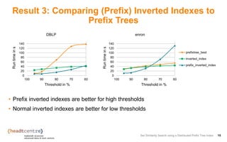
![Inverted Index (1)
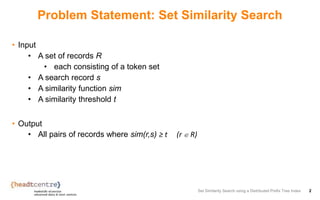
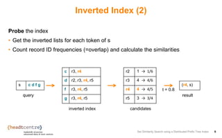
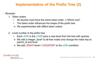
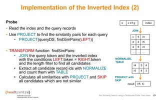
Build an inverted index {[token, {recordId}]}
Set Similarity Search using a Distributed Prefix Tree Index 5
r1 a b e
r2 a d e
r3 b c d e f g
r4 b c d f g
r5 b d f g
a r1, r2
b r1, r3, r4, r5
c r3, r4
d r2, r3, r4, r5
e r1, r2, r3
f r3, r4, r5
g r3, r4, r5](https://image.slidesharecdn.com/007fabianfier-171012203701/85/Set-Similarity-Search-using-a-Distributed-Prefix-Tree-Index-5-320.jpg)
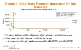
![Inverted Index (3)
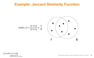
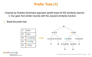
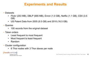
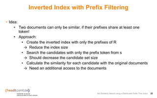
• Optimization:
• Only documents with a similar length can be similar
• Add length to the index and use it to shrink the candidate set
Set Similarity Search using a Distributed Prefix Tree Index 7
r1 a b e
r2 a d e
r3 b c d e f g
r4 b c d f g
r5 b d f g
a 3 r1, r2
b 3 r1
b 4 r5
b 5 r4
… … …
s c d f g
r4 4 → 4/5
r5 3 → 3/4
(r4, s)
query: t = 0.8, length 4 or 5
result
c 5 r4
d 4 r5
d 5 r4
f 4 r5
… … …
inverted index
{[token, length, {recordId}]}
only two
candidates
candidates
n
e
w](https://image.slidesharecdn.com/007fabianfier-171012203701/85/Set-Similarity-Search-using-a-Distributed-Prefix-Tree-Index-7-320.jpg)
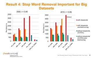


![Example
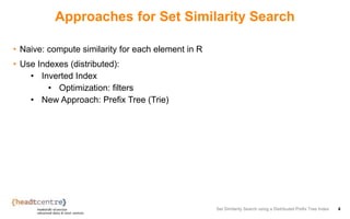
Set Similarity Search using a Distributed Prefix Tree Index 23
r1 a b e
r2 a d e
r3 b c d e f
g
r4 b c d f g
r5 b d f g
a 3 r1, r2
b 3 r1
b 4 r5
b 5 r4
… … …
s c d f g
r4 4 →
4/5
r5 3 →
3/4
(r4,
s)
t = 0.8, length 4 or 5
result
c 5 r4
d 4 r5
d 5 r4
f 4 r5
… … …
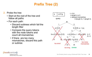
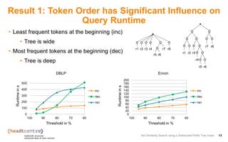
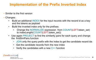
1. Build the inverted index
{[token, length, {recordId}]}
only one
candidate
2. Use the index to seach](https://image.slidesharecdn.com/007fabianfier-171012203701/85/Set-Similarity-Search-using-a-Distributed-Prefix-Tree-Index-23-320.jpg)

The document describes an approach for set similarity search using a distributed prefix tree index. It begins by introducing the problem of set similarity search and examples of similarity functions like Jaccard similarity. It then reviews existing approaches like inverted indexes and introduces a new approach using a prefix tree to index the record sets. The remainder of the document discusses implementing and testing the prefix tree approach on various datasets and analyzing the results. It finds that the token order in the prefix tree impacts performance and that adding the level as an additional index key improves query runtime. The prefix tree approach generally outperforms inverted indexes at high similarity thresholds.