Susang Kim(healess1@gmail.com)
eXplainable AI(XAI) in Computer Vision
1. CAM : Class Activation Map
2. Grad-CAM : Gradient-weighted Class Activation Mapping
3. ABN : Attention Branch Network
2.
Bias detectives
[출처] :https://www.nature.com/articles/d41586-018-05469-3
※ 회색막대기는 실재 범죄자인 경우 (붉은 칸은 AI가 범죄자로 인식)
7명중에 1명은 틀리게 예측 / 4명중에 2명은 틀리게 예측
편향된 AI는 사회적으로
많은 문제를 일으킬 수 있음
특정인을 범죄자로 인식
흑인의 얼굴 인식률의 저하
3.
eXplainable AI, XAI
[출처]: https://www.fsec.or.kr/common/proc/fsec/bbs/42/fileDownLoad/1447.do
1) XAI는 다양한 분야(Smart Factory)의 AI시스템에
사용자와 고객으로부터 신뢰 확보 가능
2) AI 모델에 대한 이해를 바탕으로 학습 모델을 설명
가능하도록 변형할 수 있고 AI 시스템의 성능 향상 가능
3) XAI를 통해 모델에 대한 원인파악이 가능하게되어 AI의
법적 책임 및 준수 확인 등의 효과가 기대
-> 딥러닝 모델 구현에 대한 근본적인 이해가 가능
설명가능한 인공지능(XAI)
기존 학습모델의 연산과정을 분석하는
방법으로 기존의 학습모델을
설명가능하도록 변형
일반적으로 통계적인 방법
(Confusion Matrix)등으로 측정을 하지만
DNN은 black box이기에 network의
output의 과정을 알 수가 없음
4.
Performance vs Explainability
[출처]: Defense Advanced Research Projects Agency https://www.darpa.mil/attachments/XAIProgramUpdate.pdf
설명이 쉬운 모델일 수록 성능은 낮은 경향을 보임 (Decision Trees -> Rdndom Forests -> DNN)
이부분에 대해 설명
5.
eXplainable AI관련 아래3개의 논문을 바탕으로 설명
Time series보다는 Vision관련 연구에 더 좋은 결과가 많음
1. Class Activation Map (CVPR 2016)
[논문] Learning deep features for discriminative localization(CVPR 2016), Bolei Zhou (MIT)
http://cnnlocalization.csail.mit.edu/Zhou_Learning_Deep_Features_CVPR_2016_paper.pdf
2. Grad-CAM (ICCV 2017)
[논문] Visual Explanations from Deep Networks via Gradient-based Localization
https://arxiv.org/pdf/1610.02391.pdf
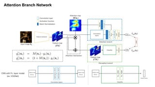
3. Attention Branch Network (CVPR 2019)
[논문] Learning of Attention Mechanism for Visual Explanation
https://arxiv.org/pdf/1812.10025.pdf
[관련논문]
Deep Inside Convolutional Networks: Visualising Image Classification Models and Saliency Maps
(ICLR 2014) https://arxiv.org/pdf/1312.6034.pdf
Prediction Difference Analysis: visualizing deep neural network decisions (ICLR 2017)
https://arxiv.org/pdf/1702.04595.pdf
FickleNet: Weakly and Semi-supervised Semantic Image Segmentation using Stochastic Inference
(CVPR 2019) https://arxiv.org/pdf/1902.10421.pdf
6.
CAM 관련 아래논문
[논문]
learning deep features for discriminative localization(CVPR 2016), Bolei Zhou (MIT)
http://cnnlocalization.csail.mit.edu/Zhou_Learning_Deep_Features_CVPR_2016_paper.pdf
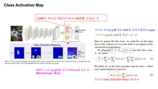
Class Activation Map
CAM의핵심은 FC대신해서 GAP를 쓰자는 것
각각의 Layer을 GAP를 통해 나온 값
각각의 위치(x,y)를 담은 GAP전 마지막 K개의 Layer
GAP의 값에 weight를 곱해 Softmax를 태운 값
(Re-training이 필요)
따라서 Class Activation Map은 M 함수
Results Caltech-UCSD Birds200 (CUB-200) is an image
dataset with photos of 200 bird species (mostly North
American). For detailed information about the dataset,
please see the technical report linked below.
■ Number of categories: 200
■ Number of images: 6,033
■ Annotations: Bounding Box, Rough
Segmentation, Attributes
0.5 IoU 기준 GAP를 거친 피쳐를 SVM으로 학습할 경우 5% 정확도가 향상
11.
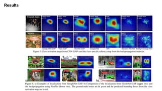
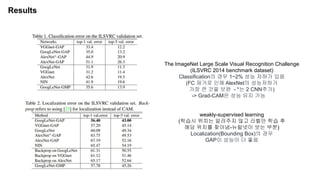
Results
The ImageNet LargeScale Visual Recognition Challenge
(ILSVRC 2014 benchmark dataset)
Classification의 경우 1~2% 성능 저허가 있음
(FC 제거로 인해 AlexNet의 성능저하가
가장 큰 것을 보완 - *는 2 CNN추가)
-> Grad-CAM은 성능 유지 가능
weakly-supervised learning
(학습시 위치는 알려주지 않고 라벨만 학습 후
해당 위치를 찾아냄-뉴럴넷이 보는 부분)
Localization(Bounding Box)의 경우
GAP이 성능이 더 좋음
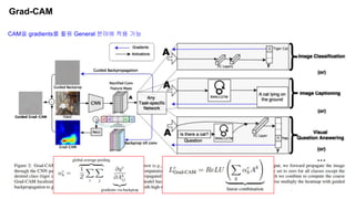
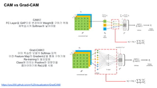
CAM vs Grad-CAM
Grad-CAM은
이미학습한 모델의 Softmax 입력
이전 Feature Map의 Gradient값을 통해 구하기에
Re-training이 필요없음
Class에 미치는 Positive한 영향만을
뽑아야하기에 ReLU를 사용
https://you359.github.io/cnn%20visualization/GradCAM/
CAM은
FC Layer을 GAP으로 변경하여 Weight를 구하기 위해
재학습시켜 Softmax에 넣어야함
CAM Code (Tensorflow)
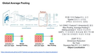
Ingeneral, for each of these networks we remove the fully-connected layers before the
final output and replace them with GAP followed by a fully-connected softmax layer.
Note that removing fully-connected layers largely decreases network parameters (e.g. 90%
less parameters for VGGnet), but also brings some classification performance drop.
def cam(_x, _W, _b, _kr):
gap = tf.nn.avg_pool(_x, ksize=[1, 28, 28, 1], strides=[1, 28, 28, 1], padding='SAME')
gap_dr = tf.nn.dropout(gap, _kr)
gap_vec = tf.reshape(gap_dr, [-1, _W['out'].get_shape().as_list()[0]])
out = tf.add(tf.matmul(gap_vec, _W['out']), _b['out'])
ret = {'x': _x, 'gap': gap, 'gap_dr': gap_dr, 'gap_vec': gap_vec, 'out': out}
return ret
https://github.com/sjchoi86/advanced-tensorflow/blob/master/cam/cam.ipynb

![Bias detectives
[출처] : https://www.nature.com/articles/d41586-018-05469-3
※ 회색막대기는 실재 범죄자인 경우 (붉은 칸은 AI가 범죄자로 인식)
7명중에 1명은 틀리게 예측 / 4명중에 2명은 틀리게 예측
편향된 AI는 사회적으로
많은 문제를 일으킬 수 있음
특정인을 범죄자로 인식
흑인의 얼굴 인식률의 저하](https://image.slidesharecdn.com/paperexplainableaixaiincomputervision-210411093712/85/Paper-eXplainable-ai-xai-in-computer-vision-2-320.jpg)
![eXplainable AI, XAI
[출처] : https://www.fsec.or.kr/common/proc/fsec/bbs/42/fileDownLoad/1447.do
1) XAI는 다양한 분야(Smart Factory)의 AI시스템에
사용자와 고객으로부터 신뢰 확보 가능
2) AI 모델에 대한 이해를 바탕으로 학습 모델을 설명
가능하도록 변형할 수 있고 AI 시스템의 성능 향상 가능
3) XAI를 통해 모델에 대한 원인파악이 가능하게되어 AI의
법적 책임 및 준수 확인 등의 효과가 기대
-> 딥러닝 모델 구현에 대한 근본적인 이해가 가능
설명가능한 인공지능(XAI)
기존 학습모델의 연산과정을 분석하는
방법으로 기존의 학습모델을
설명가능하도록 변형
일반적으로 통계적인 방법
(Confusion Matrix)등으로 측정을 하지만
DNN은 black box이기에 network의
output의 과정을 알 수가 없음](https://image.slidesharecdn.com/paperexplainableaixaiincomputervision-210411093712/85/Paper-eXplainable-ai-xai-in-computer-vision-3-320.jpg)
![Performance vs Explainability
[출처] : Defense Advanced Research Projects Agency https://www.darpa.mil/attachments/XAIProgramUpdate.pdf
설명이 쉬운 모델일 수록 성능은 낮은 경향을 보임 (Decision Trees -> Rdndom Forests -> DNN)
이부분에 대해 설명](https://image.slidesharecdn.com/paperexplainableaixaiincomputervision-210411093712/85/Paper-eXplainable-ai-xai-in-computer-vision-4-320.jpg)
![eXplainable AI관련 아래 3개의 논문을 바탕으로 설명
Time series보다는 Vision관련 연구에 더 좋은 결과가 많음
1. Class Activation Map (CVPR 2016)
[논문] Learning deep features for discriminative localization(CVPR 2016), Bolei Zhou (MIT)
http://cnnlocalization.csail.mit.edu/Zhou_Learning_Deep_Features_CVPR_2016_paper.pdf
2. Grad-CAM (ICCV 2017)
[논문] Visual Explanations from Deep Networks via Gradient-based Localization
https://arxiv.org/pdf/1610.02391.pdf
3. Attention Branch Network (CVPR 2019)
[논문] Learning of Attention Mechanism for Visual Explanation
https://arxiv.org/pdf/1812.10025.pdf
[관련논문]
Deep Inside Convolutional Networks: Visualising Image Classification Models and Saliency Maps
(ICLR 2014) https://arxiv.org/pdf/1312.6034.pdf
Prediction Difference Analysis: visualizing deep neural network decisions (ICLR 2017)
https://arxiv.org/pdf/1702.04595.pdf
FickleNet: Weakly and Semi-supervised Semantic Image Segmentation using Stochastic Inference
(CVPR 2019) https://arxiv.org/pdf/1902.10421.pdf](https://image.slidesharecdn.com/paperexplainableaixaiincomputervision-210411093712/85/Paper-eXplainable-ai-xai-in-computer-vision-5-320.jpg)
![CAM 관련 아래 논문
[논문]
learning deep features for discriminative localization(CVPR 2016), Bolei Zhou (MIT)
http://cnnlocalization.csail.mit.edu/Zhou_Learning_Deep_Features_CVPR_2016_paper.pdf](https://image.slidesharecdn.com/paperexplainableaixaiincomputervision-210411093712/85/Paper-eXplainable-ai-xai-in-computer-vision-6-320.jpg)

![CAM Code (Tensorflow)
In general, for each of these networks we remove the fully-connected layers before the
final output and replace them with GAP followed by a fully-connected softmax layer.
Note that removing fully-connected layers largely decreases network parameters (e.g. 90%
less parameters for VGGnet), but also brings some classification performance drop.
def cam(_x, _W, _b, _kr):
gap = tf.nn.avg_pool(_x, ksize=[1, 28, 28, 1], strides=[1, 28, 28, 1], padding='SAME')
gap_dr = tf.nn.dropout(gap, _kr)
gap_vec = tf.reshape(gap_dr, [-1, _W['out'].get_shape().as_list()[0]])
out = tf.add(tf.matmul(gap_vec, _W['out']), _b['out'])
ret = {'x': _x, 'gap': gap, 'gap_dr': gap_dr, 'gap_vec': gap_vec, 'out': out}
return ret
https://github.com/sjchoi86/advanced-tensorflow/blob/master/cam/cam.ipynb](https://image.slidesharecdn.com/paperexplainableaixaiincomputervision-210411093712/85/Paper-eXplainable-ai-xai-in-computer-vision-18-320.jpg)
![Grad-CAM Code (Tensorflow)
https://github.com/sjchoi86/deep-uncertainty/blob/master/code/demo_gradcam_resnet50.ipynb
eval_graph = tf.Graph()
with eval_graph.as_default():
with eval_graph.gradient_override_map({'Relu': 'GuidedRelu'}):
# if 1:
with slim.arg_scope(resnet_v1.resnet_arg_scope()):
x = tf.placeholder(tf.float32, [1, 224, 224, 3])
y = tf.placeholder(tf.float32, [1, 1000])
is_train = tf.placeholder(tf.bool)
net, end_points = resnet_v1.resnet_v1_50(x,1000,is_training=is_train)
# print end_points.keys() # print keys
logit = end_points['resnet_v1_50/logits'] # before softmax
prob = end_points['predictions'] # after softmax
conv = end_points['resnet_v1_50/block4/unit_2/bottleneck_v1']
cost = tf.reduce_sum((logit * y))
conv_grad = tf.gradients(cost, conv)[0]
conv_grad_norm = tf.div(conv_grad,
tf.sqrt(tf.reduce_mean(tf.square(conv_grad)))
+tf.constant(1e-10))
ginit = tf.global_variables_initializer()
linit = tf.local_variables_initializer()
""" Restorer """
ckpt = "net/resnet_v1_50_2016_08_28/resnet_v1_50.ckpt"
variables_to_restore = slim.get_variables_to_restore(include=["resnet_v1"])
saver = tf.train.Saver(variables_to_restore)
print ("Graph ready")](https://image.slidesharecdn.com/paperexplainableaixaiincomputervision-210411093712/85/Paper-eXplainable-ai-xai-in-computer-vision-19-320.jpg)
![ABN Code (PyTorch)
https://github.com/machine-perception-robotics-group/attention_branch_network/blob/master/models/cifar/resnet.py
https://github.com/machine-perception-robotics-group/attention_branch_network/blob/master/cifar.py
criterion = nn.CrossEntropyLoss()
optimizer = optim.SGD(model.parameters(), lr=args.lr, momentum=args.momentum, weight_decay=args.weight_decay)
for batch_idx, (inputs, targets) in enumerate(trainloader):
# measure data loading time
data_time.update(time.time() - end)
if use_cuda:
inputs, targets = inputs.cuda(), targets.cuda(async=True)
inputs, targets = torch.autograd.Variable(inputs), torch.autograd.Variable(targets)
# compute output
att_outputs, per_outputs, _ = model(inputs)
att_loss = criterion(att_outputs, targets)
per_loss = criterion(per_outputs, targets)
loss = att_loss + per_loss
# measure accuracy and record loss
prec1, prec5 = accuracy(per_outputs.data, targets.data, topk=(1, 5))
losses.update(loss.data[0], inputs.size(0))
top1.update(prec1[0], inputs.size(0))
top5.update(prec5[0], inputs.size(0))](https://image.slidesharecdn.com/paperexplainableaixaiincomputervision-210411093712/85/Paper-eXplainable-ai-xai-in-computer-vision-20-320.jpg)


![Deformable DETR Review [CDM]](https://cdn.slidesharecdn.com/ss_thumbnails/deformabledetrreviewcdm-201113070345-thumbnail.jpg?width=640&height=640&fit=bounds)


![[Paper Review] Visualizing and understanding convolutional networks](https://cdn.slidesharecdn.com/ss_thumbnails/visualizingandunderstandingconvolutionalnetworks-171116075511-thumbnail.jpg?width=640&height=640&fit=bounds)


![[Paper] GIRAFFE: Representing Scenes as Compositional Generative Neural Featu...](https://cdn.slidesharecdn.com/ss_thumbnails/papergirafferepresentingscenesascompositionalgenerativeneuralfeaturefields-210823043723-thumbnail.jpg?width=640&height=640&fit=bounds)
![[Paper] Multiscale Vision Transformers(MVit)](https://cdn.slidesharecdn.com/ss_thumbnails/papermultiscalevisiontransformers-210808092058-thumbnail.jpg?width=640&height=640&fit=bounds)
![[Paper] dynamic routing between capsules](https://cdn.slidesharecdn.com/ss_thumbnails/paperdynamicroutingbetweencapsules-210509101120-thumbnail.jpg?width=640&height=640&fit=bounds)
![[Paper] anti spoofing for face recognition](https://cdn.slidesharecdn.com/ss_thumbnails/paperanti-spoofingforfacerecognition-210508093958-thumbnail.jpg?width=640&height=640&fit=bounds)
![[Paper] attention mechanism(luong)](https://cdn.slidesharecdn.com/ss_thumbnails/paperattentionmechanismluong-210508090926-thumbnail.jpg?width=640&height=640&fit=bounds)
![[Paper] shuffle net an extremely efficient convolutional neural network for ...](https://cdn.slidesharecdn.com/ss_thumbnails/papershufflenetanextremelyefficientconvolutionalneuralnetworkformobiledevices-210424000132-thumbnail.jpg?width=640&height=640&fit=bounds)
![[Paper] EDA : easy data augmentation techniques for boosting performance on t...](https://cdn.slidesharecdn.com/ss_thumbnails/paperedaeasydataaugmentationtechniquesforboostingperformanceontextclassificationtasks-210414133327-thumbnail.jpg?width=640&height=640&fit=bounds)
![[Paper] auto ml part 1](https://cdn.slidesharecdn.com/ss_thumbnails/paperautomlpart1-210413122952-thumbnail.jpg?width=640&height=640&fit=bounds)
![[Paper] learning video representations from correspondence proposals](https://cdn.slidesharecdn.com/ss_thumbnails/paperlearningvideorepresentationsfromcorrespondenceproposals-210410235049-thumbnail.jpg?width=640&height=640&fit=bounds)
![[Paper] DetectoRS for Object Detection](https://cdn.slidesharecdn.com/ss_thumbnails/paperdetectorsobjectdetection-210320013551-thumbnail.jpg?width=640&height=640&fit=bounds)


