Downloaded 3,489 times


![Function Point Analysis
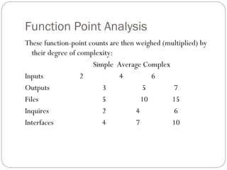
Continuing our example . . .
Complex internal processing = 3
Code to be reusable = 2
High performance = 4
Multiple sites = 3
Distributed processing = 5
Project adjustment factor = 17
Adjustment calculation:
Adjusted FP = Unadjusted FP X [0.65 + (adjustment factor X 0.01)]
= 240 X [0.65 + ( 17 X 0.01)]
= 240 X [0.82]
= 197 Adjusted function points](https://image.slidesharecdn.com/cocomomodel-130715000002-phpapp01/85/Cocomo-model-18-320.jpg)
![Function Point Analysis
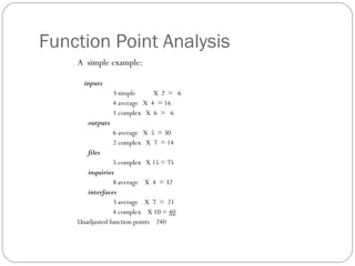
But how long will the project take and how much will it cost?
As previously measured, programmers in our organization
average 18 function points per month. Thus . . .
197 FP divided by 18 = 11 man-months
If the average programmer is paid $5,200 per month
(including benefits), then the [labor] cost of the project will
be . . .
11 man-months X $5,200 = $57,200](https://image.slidesharecdn.com/cocomomodel-130715000002-phpapp01/85/Cocomo-model-19-320.jpg)

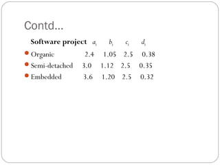
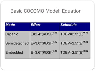
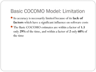
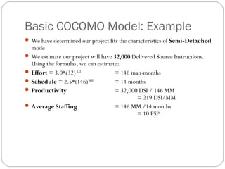
The COCOMO model is a widely used software cost estimation model developed by Barry Boehm in 1981. It predicts effort, schedule, and staffing needs based on project size and characteristics. The Basic COCOMO model uses three development modes (Organic, Semidetached, Embedded) and a simple formula to estimate effort and schedule based on thousands of delivered source instructions. However, its accuracy is limited as it does not account for various project attributes known to influence costs. Function Point Analysis is an alternative size measurement that counts different types of system functions and complexity factors to estimate effort and cost.