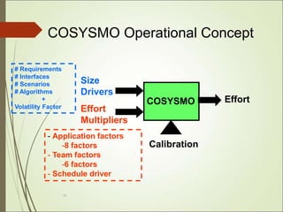
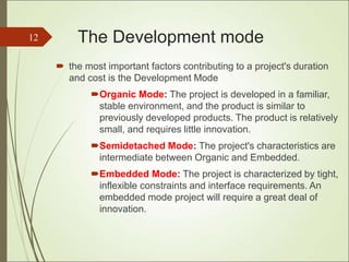
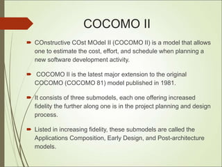
The document outlines the Cocomo (Constructive Cost Model) framework, which is widely used for software cost estimation, detailing its different models (Cocomo 1, Cocomo 2, and Cosysmo) and their applications. It emphasizes the significance of accurate cost estimation in software project management, identifying factors that affect cost, including project size and development mode. Additionally, it discusses the advantages and disadvantages of each model, ultimately providing case studies for cost estimation and project planning.

1. COCOMO
Constructive Cost Model
Vinodh Kumar Mohan, R.No : 102
Yash Deep Pandey, R.No : 103
Mohit Mahant, R.No : 104
Diana Purushotaman, R.No.105
Karthik B, R.No: 106
Prakar Rastogi, R.No: 107
1

2. Agenda
 Need for cost estimation
 Factors contributing to cost of a project
 COCOMO1
 Live project Example
 Advantages and Disadvantages
 COCOMO 2
 Advantages and Disadvantages
 Cosysmo
 Advantages and Disadvantages
2

3. Need for cost estimation
The software cost estimation provides:
 the vital link between the general concepts
and techniques of economic analysis and
the particular world of software
engineering.
 Software cost estimation techniques also
provides an essential part of the foundation
for good software management.
3

4. Cost of a project
 The factors that affect cost of a project is due to:
the requirements for software, hardware and
human resources
the cost of software development is due to the
human resources needed
most cost estimates are measured in person-
months (PM)
the cost of the project depends on the nature and
characteristics of the project, at any point, the
accuracy of the estimate will depend on the
amount of reliable information we have about the
final product.
4

5. Software Cost Estimation
5

6. COCOMO models
 The COstructive COst Model (COCOMO)
is the most widely used software estimation
model in the world. It
 The COCOMO model predicts the effort and
duration of a project based on inputs
relating to the size of the resulting systems
and a number of "cost drives" that affect
productivity.
6

7. Effort
 Effort Equation
Effort = a * (KLOC)b (person-months)
where Effort = number of person-
month (=152 working hours),
a = a constant,
KLOC = thousands of “lines of code"
(LOC) and
 b = a constant.
7

8. Productivity
 Productivity equation
(KLOC) / (Effort)
where Effort = number of person-
month (=152 working hours),
8

9. Schedule
 Schedule equation
Duration, D = C * (E)d (months)
where D = number of months
estimated for software development.
9

10. Average Staffing
 Average Staffing Equation
(Effort) / (D) (FSP)
where FSP means Full-time-
equivalent Software Personnel.
10

11. COCOMO Models
 COCOMO is defined in terms of three
different models:
the Basic model,
the Intermediate model, and
the Detailed model.
 The more complex models account for more
factors that influence software projects, and
make more accurate estimates.
11

12. The Development mode
 the most important factors contributing to a project's duration
and cost is the Development Mode
Organic Mode: The project is developed in a familiar,
stable environment, and the product is similar to
previously developed products. The product is relatively
small, and requires little innovation.
Semidetached Mode: The project's characteristics are
intermediate between Organic and Embedded.
Embedded Mode: The project is characterized by tight,
inflexible constraints and interface requirements. An
embedded mode project will require a great deal of
innovation.
12

13. Modes
Feature Organic Semidetached Embedded
Organizational
understanding of
product and
objectives
Thorough Considerable General
Experience in
working with related
software systems
Extensive Considerable Moderate
Need for software
conformance with
pre-established
requirements
Basic Considerable Full
Need for software
conformance with
external interface
specifications
Basic Considerable Full
13

14. Modes (.)
Feature Organic Semidetached Embedded
Concurrent
development of
associated new
hardware and
operational
procedures
Some Moderate Extensive
Need for innovative
data processing
architectures,
algorithms
Minimal Some Considerable
Premium on early
completion
Low Medium High
Product size range <50 KDSI <300KDSI All
14

15. Cost Estimation Process
15
Errors
Effort
Development Time
Size Table
Lines of Code
Number of Use Case
Function Point
Estimation Process
Number of Personnel
Cost=SizeOfTheProject x Productivity

16. Project Size - Metrics
1. Number of functional requirements
2. Cumulative number of functional and non-functional requirements
3. Number of Customer Test Cases
4. Number of ‘typical sized’ use cases
5. Number of inquiries
6. Number of files accessed (external, internal, master)
7. Total number of components (subsystems, modules, procedures,
routines, classes, methods)
8. Total number of interfaces
9. Number of System Integration Test Cases
10. Number of input and output parameters (summed over each interface)
11. Number of Designer Unit Test Cases
12. Number of decisions (if, case statements) summed over each routine or
method
13. Lines of Code, summed over each routine or method
16

17. Function Points
 STEP 1: measure size in terms of the amount of
functionality in a system. Function points are
computed by first calculating an unadjusted
function point count (UFC). Counts are made for
the following categories
 External inputs – those items provided by the user that describe distinct
application-oriented data (such as file names and menu selections)
 External outputs – those items provided to the user that generate distinct
application-oriented data (such as reports and messages, rather than the
individual components of these)
  External inquiries – interactive inputs requiring a response
  External files – machine-readable interfaces to other systems
  Internal files – logical master files in the system
17

18. Function Points(..)
 STEP 2: Multiply each number by a weight
factor, according to complexity (simple,
average or complex) of the parameter,
associated with that number. The value is
given by a table:
18

19. Function Points(...)
 STEP 3: Calculate the total UFP
(Unadjusted Function Points)
 STEP 4: Calculate the total TCF (Technical
Complexity Factor) by giving a value
between 0 and 5 according to the
importance of the following points:
19

20. Function Points(....)
Technical Complexity Factors:
 1. Data Communication
 2. Distributed Data Processing
 3. Performance Criteria
 4. Heavily Utilized Hardware
 5. High Transaction Rates
 6. Online Data Entry
 7. Online Updating
 8. End-user Efficiency
 9. Complex Computations
 10. Reusability
 11. Ease of Installation
 12. Ease of Operation
 13. Portability
 14. Maintainability
20

21. Function Points(.....)
 STEP 5: Sum the resulting numbers too
obtain DI (degree of influence)
 STEP 6: TCF (Technical Complexity Factor)
by given by the formula
 TCF=0.65+0.01*DI
 STEP 6: Function Points are by given by the
formula
 FP=UFP*TCF
21

22. Example
22

23. Example (.)
23

24. Example (..)
Technical Complexity Factors:
 1. Data Communication 3
 2. Distributed Data Processing 0
 3. Performance Criteria 4
 4. Heavily Utilized Hardware 0
 5. High Transaction Rates 3
 6. Online Data Entry 3
 7. Online Updating 3
 8. End-user Efficiency 3
 9. Complex Computations 0
 10. Reusability 3
 11. Ease of Installation 3
 12. Ease of Operation 5
 13. Portability 3
 14. Maintainability 3
 DI =30 (Degree of Influence)
24

25. Example (…)
 Function Points
 FP=UFP*(0.65+0.01*DI)= 55*(0.65+0.01*30)=52.25
 That means the is FP=52.25
25

26. Relation between LOC and FP
 Relationship:
 LOC = Language Factor * FP
 where
 LOC (Lines of Code)
 FP (Function Points)
26

27. Relation between LOC and
FP(.)
Assuming LOC’s per FP for:
Java = 53,
C++ = 64
aKLOC = FP * LOC_per_FP / 1000
It means for the SpellChekcer Example: (Java)
LOC=52.25*53=2769.25 LOC or 2.76 KLOC
27

28. Effort Computation
 The Basic COCOMO model computes
effort as a function of program size. The
Basic COCOMO equation is:
 E = aKLOC^b
 Effort for three modes of Basic COCOMO.
28
Mode a b
Organic 2.4 1.05
Semi-
detached
3.0 1.12
Embedded 3.6 1.20

29. Example
29

30. Effort Computation
 The intermediate COCOMO model
computes effort as a function of program
size and a set of cost drivers. The
Intermediate COCOMO equation is:
 E = aKLOC^b*EAF
 Effort for three modes of intermediate
COCOMO.
30
Mode a b
Organic 3.2 1.05
Semi-
detached
3.0 1.12
Embedded 2.8 1.20

31. Effort computation(.)
 Effort Adjustment Factor
31
Cost Driver Very
Low
Low Nominal High Very
High
Extra
High
Required Reliability .75 .88 1.00 1.15 1.40 1.40
Database Size .94 .94 1.00 1.08 1.16 1.16
Product Complexity .70 .85 1.00 1.15 1.30 1.65
Execution Time Constraint 1.00 1.00 1.00 1.11 1.30 1.66
Main Storage Constraint 1.00 1.00 1.00 1.06 1.21 1.56
Virtual Machine Volatility .87 .87 1.00 1.15 1.30 1.30
Comp Turn Around Time .87 .87 1.00 1.07 1.15 1.15
Analyst Capability 1.46 1.19 1.00 .86 .71 .71
Application Experience 1.29 1.13 1.00 .91 .82 .82
Programmers Capability 1.42 1.17 1.00 .86 .70 .70
Virtual machine Experience 1.21 1.10 1.00 .90 .90 .90
Language Experience 1.14 1.07 1.00 .95 .95 .95
Modern Prog Practices 1.24 1.10 1.00 .91 .82 .82
SW Tools 1.24 1.10 1.00 .91 .83 .83
Required Dev Schedule 1.23 1.08 1.00 1.04 1.10

32. Effort Computation (..)
Total EAF = Product of the selected factors
Adjusted value of Effort: Adjusted Person
Months:
APM = (Total EAF) * PM
 PM – Person Months
32

33. Example
33

34. Software Development Time
 Development Time Equation Parameter
Table:
Development Time, TDEV = C * (APM^D)
Number of Personnel, NP = APM / TDEV
34
Parameter Organic Semi-
detached
Embedded
C 2.5 2.5 2.5
D 0.38 0.35 0.32

35. Distribution of Effort (.)
The following table gives the recommended percentage
distribution of Effort (APM) and TDEV for these
stages:
Percentage Distribution of Effort and Time Table:
35
Req
Analysis
Design,
HLD + DD
Implementation Testing
Effort 23% 29% 22% 21% 100%
TDEV 39% 25% 15% 21% 100%

36. Advantages and
Disadvantages
 Advantage
 COCOMO is transparent, one can see how it works unlike
other models.
 Drivers are particularly helpful to the estimator to understand
the impact of different factors that affect project costs
 Disadvantages
 It is hard to accurately estimate KLOC early on in the project,
when most effort estimates are required
 Extremely vulnerable to mis-classification of the development
mode
 Success depends largely on tuning the model to the needs of
the organization, using historical data which is not always
available
36

37. COCOMO II
 COnstructive COst MOdel II (COCOMO II) is a model that allows
one to estimate the cost, effort, and schedule when planning a
new software development activity.
 COCOMO II is the latest major extension to the original
COCOMO (COCOMO 81) model published in 1981.
 It consists of three submodels, each one offering increased
fidelity the further along one is in the project planning and design
process.
 Listed in increasing fidelity, these submodels are called the
Applications Composition, Early Design, and Post-architecture
models.

38. Applications
 Making investment or other financial decisions
involving a software development effort
 Setting project budgets and schedules as a basis for
planning and control
 Deciding on or negotiating tradeoffs among software
cost, schedule, functionality, performance or quality
factors
 Making software cost and schedule risk management
decisions
 Deciding which parts of a software system to
develop, reuse, lease, or purchase
 Making legacy software inventory decisions: what
parts to modify, phase out, outsource, etc

39. Project Description and
Scope
 A bioinformatics company, providing advanced
methods for data mining of genetic information, intends
to construct a distributed application for analysis and
navigation of biological networks
 As part of this project, a database provider that
exposes simple interfaces to UI programmer and hides
complexities of the data layer should be build
 As soon as the scope of this task is broadly defined as
such, it is sliced into a separate project

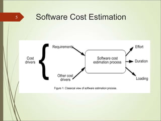
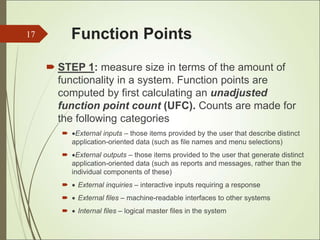
40. COCOMO II Estimates
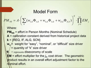
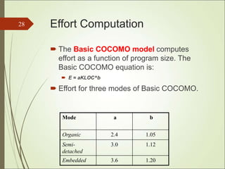
The basic COCOMO equations take the form
 Effort Applied (E) = ab(KLOC)b
b [ person-months ]
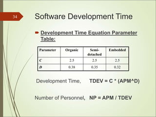
 Development Time (D) = cb(Effort Applied)d
b [months]
 People required (P) = Effort Applied / Development
Time [count]
Software
Project
ab bb cb db
Organic 2.4 1.05 2.5 0.38
Semi-
Detached
3.0 1.12 2.5 0.35
Embedded 3.6 1.20 2.5 0.32

41. Counting SLOC in the Project
 To make actual estimations, SLOC count
needs to be figured out for each of the
components and use these counts in
COCOMO model.
 The result of separate SLOC count in all
project folders is the following:
Folder Total SLOC
1 SQL Files 414
2 Java DB Provider Files 345
3 Java Servlet 156
4 Web Files 113

42. Final Cost Estimates and
Results
The report says that project cost is $23,000 and project
duration is 4.6 months ($5000 was taken as an average
monthly developer salary)

43. Merits & De-merits
Merits:
 COCOMO II is an industry standard
 Very profound information is easy available
 Clear and effective calibration process by combining delphi with
algorithmic cost estimation techniques
 Backwards compatibility' with the Rosetta Stone
 Various extension for almost every purpose are available
 Tool support
De-Merits:
 The 'heart' of COCOMO II is still based on a waterfall process
model
 Most of the extensions are still experimental and not fully
calibrated till now
 Duration calculation for small projects is unreasonable

44. 44
COSYSMO Overview
• Parametric model to estimate System Engineering costs
• Includes 4 size drivers (# Requirements, # Interfaces, # Operational
Scenarios, # algorithms) & 14 cost drivers (Req understanding,
Technology maturity, Process capability, Personnel experience, Tool
Support, etc.)
• Supports Local Calibration (based on historical project data)
• Developed with USC-Center for Software Engineering Corporate Affiliates,
Practical Software Measurement (PSM), and INCOSE participation
Conceptualize Develop
Oper Test
& Eval
Transition
to
Operation
Operate,
Maintain,
or
Enhance
Replace
or
Dismantle
Supported by Initial Model
calibration and release
These phases are not currently supported

45. 45
COSYSMO
Size
Drivers
Effort
Multipliers
Effort
Calibration
# Requirements
# Interfaces
# Scenarios
# Algorithms
+
Volatility Factor
- Application factors
-8 factors
- Team factors
-6 factors
- Schedule driver
COSYSMO Operational Concept

46. 46
Where:
PMNS = effort in Person Months (Nominal Schedule)
A = calibration constant derived from historical project data
k = {REQ, IF, ALG, SCN}
wx = weight for “easy”, “nominal”, or “difficult” size driver
= quantity of “k” size driver
E = represents diseconomy of scale
EM = effort multiplier for the jth cost driver. The geometric
product results in an overall effort adjustment factor to the
nominal effort.
x

Model Form

 
















14
1
,
,
,
,
,
, )
(
j
j
E
k
k
d
k
d
k
n
k
n
k
e
k
e
NS EM
w
w
w
A
PM

47. 47
4 Size Drivers
1. Number of System Requirements*
2. Number of System Interfaces
3. Number of System Specific Algorithms
4. Number of Operational Scenarios
*Weighted by complexity, volatility, and degree of reuse

48. 48
14 Cost Drivers
1. Requirements understanding
2. Architecture understanding
3. Level of service requirements
4. Migration complexity
5. Technology Maturity
6. Documentation Match to Life Cycle Needs
7. # and Diversity of Installations/Platforms
8. # of Recursive Levels in the Design
Application Factors (8)

49. 49
14 Cost Drivers (cont.)
1. Stakeholder team cohesion
2. Personnel/team capability
3. Personnel experience/continuity
4. Process capability
5. Multisite coordination
6. Tool support
Team Factors (6)

50. Advantages and
Disadvantages
Advantages
 More accurate method for effort estimation
 Includes specific calibrations for different industries and
types of project
Disadvantages
 The disadvantages are that this process is labor intensive
and is typically not uniform across entities.
 every level folds in another layer of conservative
management reserve which can result in an over estimate
at the end.
50

51. THANK YOU!
51