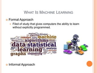
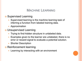
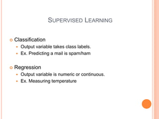
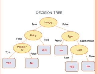
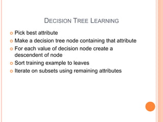
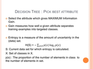
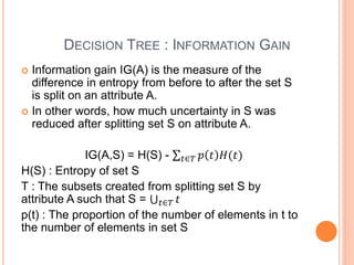
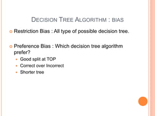
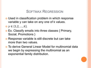
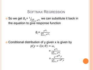
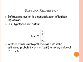
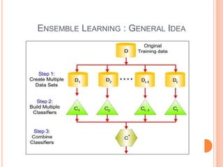
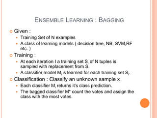
DECISION TREE, SOFTMAX 
REGRESSION AND ENSEMBLE 
METHODS IN MACHINE LEARNING 
- Abhishek Vijayvargia
WHAT IS MACHINE LEARNING 
 Formal Approach 
 Filed of study that gives computers the ability to learn 
without explicitly programmed. 
 Informal Approach
MACHINE LEARNING 
 Supervised Learning 
 Supervised learning is the machine learning task of 
inferring a function from labeled training data. 
 Approximation 
 Unsupervised Learning 
 Trying to find hidden structure in unlabeled data. 
 Examples given to the learner are unlabeled, there is no 
error or reward signal to evaluate a potential solution. 
 Shorter Description 
 Reinforcement learning 
 Learning by interacting with an environment
SUPERVISED LEARNING 
 Classification 
 Output variable takes class labels. 
 Ex. Predicting a mail is spam/ham 
 Regression 
 Output variable is numeric or continuous. 
 Ex. Measuring temperature
DECISION TREES 
 Is this restaurant good? 
 ( YES/ NO)
DECISION TREES 
 What are the factors which decide that restaurant is 
good for you or not? 
 Type : Italian, South Indian, French 
 Atmosphere: Casual, Fancy 
 How many people inside it? (10< people > 30 ) 
 Cost 
 Weather outside : Rainy, Sunny, Cloudy 
 Hungry : Yes/No
DECISION TREE 
Hungry 
True False 
Rainy 
People > 
10 
YES No 
YES 
Type 
Cost 
YES No 
No 
True 
False 
True 
False 
French South Indian 
More 
Less
DECISION TREE LEARNING 
 Pick best attribute 
 Make a decision tree node containing that attribute 
 For each value of decision node create a 
descendent of node 
 Sort training example to leaves 
 Iterate on subsets using remaining attributes
DECISION TREE : PICK BEST ATTRIBUTE 
True 
+ + - 
+ + - - 
+ -+- 
False 
- - + - 
+ - + 
+ - - + 
True 
+ - + - 
+ + + 
- - - + 
False 
True 
+ + + 
+ + 
False 
- - - - 
- - - 
Graph. 1 Graph. 2 Graph. 3
DECISION TREE : PICK BEST ATTRIBUTE 
 Select the attribute which gives MAXIMUM Information 
Gain. 
 Gain measures how well a given attribute separates 
training examples into targeted classes. 
 Entropy is a measure of the amount of uncertainty in the 
(data) set. 
H(S) = − 푥∈푋 푝(푥) log2 푝(푥) 
S: Current data set for which entropy is calculated. 
X: Set of classes in X. 
p(x) : The proportion of the number of elements in class to 
the number of elements in set.
DECISION TREE : INFORMATION GAIN 
 Information gain IG(A) is the measure of the 
difference in entropy from before to after the set S 
is split on an attribute A. 
 In other words, how much uncertainty in S was 
reduced after splitting set S on attribute A. 
IG(A,S) = H(S) - 푡∈푇 푝 푡 퐻(푡) 
H(S) : Entropy of set S 
T : The subsets created from splitting set S by 
attribute A such that S = 푡∈푇 푡 
p(t) : The proportion of the number of elements in t to 
the number of elements in set S
DECISION TREE ALGORITHM : BIAS 
 Restriction Bias : All type of possible decision tree. 
 Preference Bias : Which decision tree algorithm 
prefer? 
 Good split at TOP 
 Correct over Incorrect 
 Shorter tree
DECISION TREE : CONTINUOUS ATTRIBUTE 
 Branch on number of possible values? 
 Include age only in training set? 
 Useless when we get some age not present in training 
set 
 Represent in the form of range 
Age 
1.11 1.111 
20<=Age<30
DECISION TREE : CONTINUOUS ATTRIBUTE 
 Does it make sense to repeat an attribute along a 
path in the tree? 
B 
A A 
A 
B 
A
DECISION TREE : WHEN DO WE STOP? 
 Everything classified correctly? (same example/ 
noisy two answer for same) 
 No more attribute? ( not good for continuous 
attribute/ infinite possibility) 
 Pruning
SOFTMAX REGRESSION 
 Softmax Regression ( or multinomial logistic 
regression) is a classification method that 
generalizes logistic regression to multiclass 
problems. (i.e. with more than two possible discrete 
outcomes.) 
 Used to predict the probabilities of the different 
possible outcomes of a categorically distributed 
dependent variable, given a set of independent 
variables (which may be real-valued, binary-valued, 
categorical-valued, etc.).
LOGISTIC REGRESSION 
 Logistic regression is used to refer specifically to 
the problem in which the dependent variable is 
binary ( only two categories). 
 As output variable y ∈ 0,1 , it seems natural to 
choose Bernoulli family of distribution to model 
conditional distribution of y given x. 
 Logistic function (which always takes on values 
between zero and one) 
퐹 푡 = 1 
1+푒−푡 = 1 
푒−휃푇푥
SOFTMAX REGRESSION 
 Used in classification problem in which response 
variable y can take on any one of k values. 
 푦 ∈ 1,2, … , 푘 . 
 Ex. Classify emails into three classes { Primary, 
Social, Promotions } 
 Response variable is still discrete but can take 
more than two values. 
 To derive General Linear Model for multinomial data 
we begin by expressing the multinomial as an 
exponential family distribution.
SOFTMAX REGRESSION 
 To parameterize a multinomial over k-possible 
outcomes, we could use k parameters ∅1, … , ∅푘 
specifying probability of each outcomes. 
푘 ∅푖 = 
 These parameters are redundant because 푖=1 
1. So ∅푖 = 푝 푦 = 푖; ∅ 
푘 ∅푖 
 and 푝(푦 = 푘; ∅) = 1 − 푖=1 
 Indicator Function 1{.} takes a value of 1 if it’s 
argument is true, and 0 otherwise. 
 1{True} = 1, 1{False} = 0.
SOFTMAX REGRESSION 
 Multinomial is member of exponential family. 
1{푦=1} ∅2 
푝 푦; ∅ = ∅1 
1{푦=2} … … . ∅푘 
1{푦=푘} 
1{푦=1} ∅2 
= ∅1 
1− 푖=1 
1{푦=2} … … . ∅푘 
푘−1{푦=푖} 
=푏 푦 exp 휔푇 푇 푦 − a ω 
Where 휔 = 
log ∅ 1 ∅푘 
log ∅ 2 ∅푘 
⋮ 
log ∅ 푘 − 1 ∅푘 
푎 휔 = − log ∅푘 
푏 푦 = 1 푇 푦 ∈ 푅푘 
_1
SOFTMAX REGRESSION 
 The link function is given as 
휔푖 = log 
∅푖 
∅푘 
To invert the link function and derive the response 
function 
푒휔푖 = 
∅푖 
∅푘 
∅푘푒휔푖 = ∅푖 
∅푘 
푘 
푖=1 
푒휔푖 = 
푘 
푖=1 
∅푖 = 1
SOFTMAX REGRESSION 
 So we get ∅푘= 1 
푘 푒휔 
푖=1 
푖 
we can substitute it back in 
the equation to give response function 
∅푖= 
푒휔 
푖 
푘 푒휔 
푖=1 
푖 
 Conditional distribution of y given x is given by 
푝 푦 = 푖 푥; 휃 = 휔푖 
= 
푒휔 
푖 
푘 푒휔 
푖=1 
푖 
= 
푒−휃푖푇 
푥 
푖 
푘 푒−휃푇 
푖=1 
푥 
푖
SOFTMAX REGRESSION 
 Softmax regression is a generalization of logistic 
regression. 
 Our Hypothesis will output 
ℎ휃 푥 = 
∅1 
∅2 
⋮ 
∅푘 
 In other words, our hypothesis will output the 
estimated probability 푝 푦 = 푖 푥; 휃 for every value of 
i = 1, .. k.
ENSEMBLE LEARNING 
 Ensemble learning use multiple learning algorithms 
to obtain better predictive performance than could 
be obtained from any of the constituent learning 
algorithms. 
 Ensemble learning is primarily used to improve the 
prediction performance of a model, or reduce the 
likelihood of an unfortunate selection of a poor one.
HOW GOOD ARE ENSEMBLES? 
 Let’s look at NetFlix Prize Competition…
NETFLIX PRIZE : STARTED IN OCT 2006 
 Supervised Learning Task 
 Training Data is a set of users and rating (1,2,3,4,5 
stars) those users have given to movies. 
 Construct a classifier that given a user and an unrated 
movie, correctly classified that movie as either 1,2,3,4 or 
5 stars. 
 $1 Million prize for a 10% improvement over Netflix 
current movie recommender/Classifier.
NETFLIX PRIZE : LEADER BOARD
ENSEMBLE LEARNING : GENERAL IDEA
ENSEMBLE LEARNING : BAGGING 
 Given : 
 Training Set of N examples 
 A class of learning models ( decision tree, NB, SVM,RF 
etc. ) 
 Training : 
 At each iteration I a training set Si of N tuples is 
sampled with replacement from S. 
 A classifier model Mi is learned for each training set Si. 
 Classification : Classify an unknown sample x 
 Each classifier Mi returns it’s class prediction. 
 The bagged classifier M* count the votes and assign the 
class with the most votes.
ENSEMBLE LEARNING : BAGGING 
 Bagging reduces variance by voting/averaging. 
 Can help a lot when data is noisy. 
 If learning algorithm is unstable, then Bagging 
almost always improves performance.
ENSEMBLE LEARNING : RANDOM FORESTS 
 Random Forests grows many classification trees. 
 To classify a new object from an input vector, put 
the input vector down each of the trees in the 
forest. 
 Each tree gives a classification, and we say the tree 
"votes" for that class. 
 The forest chooses the classification having the 
most votes (over all the trees in the forest).
ENSEMBLE LEARNING : RANDOM FORESTS 
 Each tree is grown as follows: 
 If the number of cases in the training set is N, 
sample N cases at random - but with replacement, 
from the original data. This sample will be the 
training set for growing the tree. 
 If there are M input variables, a number m<<M is 
specified such that at each node, m variables are 
selected at random out of the M and the best split 
on these m is used to split the node. The value of m 
is held constant during the forest growing. 
 Each tree is grown to the largest extent possible. 
There is no pruning.
FEATURES OF RANDOM FORESTS 
 Better in accuracy among current algorithms. 
 Runs efficiently on large data bases. 
 It can handle thousands of input variables without 
variable deletion. 
 It gives estimates of what variables are important in 
the classification. 
 Effective method for estimating missing data and 
maintains accuracy when a large proportion of the 
data are missing. 
 Generated forests can be saved for future use on 
other data.
ENSEMBLE LEARNING : BOOSTING 
 Create a sequence of classifiers, giving higher 
influence to more accurate classifiers. 
 At each iteration, make examples currently 
misclassified more important( get larger weight in 
the construction of the next classifier) 
 Then combine classifier by weighted vote (weight 
given by classifier accuracy)
ENSEMBLE LEARNING : BOOSTING 
 Suppose there are just 7 training examples 
{1,2,3,4,5,6,7} 
 Initially each example has a 0.142 (1/7) probability of 
being sampled. 
 1st round of boosting samples ( with replacement) 7 
examples { 3,5,5,4,6,7,3} and build a classifier from 
them. 
 Suppose examples {2,3,4,6,7} are correctly predicted by 
this classifier and examples {1,5} are wrongly predicted: 
 Weight of examples {1,5} are increased. 
 Weight of examples {2,3,4,6,7} are decreased. 
 2nd round of boosting again take 7 examples, but now 
examples {1,5} are more likely to be sampled. 
 And so on until some convergence is achieved.
ENSEMBLE LEARNING : BOOSTING 
 Weights models according to performance. 
 Encourage new model to become an “expert” for 
instances misclassified by earlier model. 
 Combines “Weak Learner” to generate “strong 
learner”.
ENSEMBLE LEARNING 
 Netflix 1st prize winner gradient boosted decision 
tree. 
 http://www.netflixprize.com/assets/GrandPrize2009 
_BPC_BellKor.pdf
THANK YOU FOR YOUR ATTENTION
 Ask Question to narrow down possiblity 
 Informatica building example 
 Mango machine learning 
 Cannot look all trees

Decision tree, softmax regression and ensemble methods in machine learning

  • 1.
    DECISION TREE, SOFTMAX REGRESSION AND ENSEMBLE METHODS IN MACHINE LEARNING - Abhishek Vijayvargia
  • 2.
    WHAT IS MACHINELEARNING  Formal Approach  Filed of study that gives computers the ability to learn without explicitly programmed.  Informal Approach
  • 3.
    MACHINE LEARNING Supervised Learning  Supervised learning is the machine learning task of inferring a function from labeled training data.  Approximation  Unsupervised Learning  Trying to find hidden structure in unlabeled data.  Examples given to the learner are unlabeled, there is no error or reward signal to evaluate a potential solution.  Shorter Description  Reinforcement learning  Learning by interacting with an environment
  • 4.
    SUPERVISED LEARNING Classification  Output variable takes class labels.  Ex. Predicting a mail is spam/ham  Regression  Output variable is numeric or continuous.  Ex. Measuring temperature
  • 5.
    DECISION TREES Is this restaurant good?  ( YES/ NO)
  • 6.
    DECISION TREES What are the factors which decide that restaurant is good for you or not?  Type : Italian, South Indian, French  Atmosphere: Casual, Fancy  How many people inside it? (10< people > 30 )  Cost  Weather outside : Rainy, Sunny, Cloudy  Hungry : Yes/No
  • 7.
    DECISION TREE Hungry True False Rainy People > 10 YES No YES Type Cost YES No No True False True False French South Indian More Less
  • 8.
    DECISION TREE LEARNING  Pick best attribute  Make a decision tree node containing that attribute  For each value of decision node create a descendent of node  Sort training example to leaves  Iterate on subsets using remaining attributes
  • 9.
    DECISION TREE :PICK BEST ATTRIBUTE True + + - + + - - + -+- False - - + - + - + + - - + True + - + - + + + - - - + False True + + + + + False - - - - - - - Graph. 1 Graph. 2 Graph. 3
  • 10.
    DECISION TREE :PICK BEST ATTRIBUTE  Select the attribute which gives MAXIMUM Information Gain.  Gain measures how well a given attribute separates training examples into targeted classes.  Entropy is a measure of the amount of uncertainty in the (data) set. H(S) = − 푥∈푋 푝(푥) log2 푝(푥) S: Current data set for which entropy is calculated. X: Set of classes in X. p(x) : The proportion of the number of elements in class to the number of elements in set.
  • 11.
    DECISION TREE :INFORMATION GAIN  Information gain IG(A) is the measure of the difference in entropy from before to after the set S is split on an attribute A.  In other words, how much uncertainty in S was reduced after splitting set S on attribute A. IG(A,S) = H(S) - 푡∈푇 푝 푡 퐻(푡) H(S) : Entropy of set S T : The subsets created from splitting set S by attribute A such that S = 푡∈푇 푡 p(t) : The proportion of the number of elements in t to the number of elements in set S
  • 12.
    DECISION TREE ALGORITHM: BIAS  Restriction Bias : All type of possible decision tree.  Preference Bias : Which decision tree algorithm prefer?  Good split at TOP  Correct over Incorrect  Shorter tree
  • 13.
    DECISION TREE :CONTINUOUS ATTRIBUTE  Branch on number of possible values?  Include age only in training set?  Useless when we get some age not present in training set  Represent in the form of range Age 1.11 1.111 20<=Age<30
  • 14.
    DECISION TREE :CONTINUOUS ATTRIBUTE  Does it make sense to repeat an attribute along a path in the tree? B A A A B A
  • 15.
    DECISION TREE :WHEN DO WE STOP?  Everything classified correctly? (same example/ noisy two answer for same)  No more attribute? ( not good for continuous attribute/ infinite possibility)  Pruning
  • 16.
    SOFTMAX REGRESSION Softmax Regression ( or multinomial logistic regression) is a classification method that generalizes logistic regression to multiclass problems. (i.e. with more than two possible discrete outcomes.)  Used to predict the probabilities of the different possible outcomes of a categorically distributed dependent variable, given a set of independent variables (which may be real-valued, binary-valued, categorical-valued, etc.).
  • 17.
    LOGISTIC REGRESSION Logistic regression is used to refer specifically to the problem in which the dependent variable is binary ( only two categories).  As output variable y ∈ 0,1 , it seems natural to choose Bernoulli family of distribution to model conditional distribution of y given x.  Logistic function (which always takes on values between zero and one) 퐹 푡 = 1 1+푒−푡 = 1 푒−휃푇푥
  • 18.
    SOFTMAX REGRESSION Used in classification problem in which response variable y can take on any one of k values.  푦 ∈ 1,2, … , 푘 .  Ex. Classify emails into three classes { Primary, Social, Promotions }  Response variable is still discrete but can take more than two values.  To derive General Linear Model for multinomial data we begin by expressing the multinomial as an exponential family distribution.
  • 19.
    SOFTMAX REGRESSION To parameterize a multinomial over k-possible outcomes, we could use k parameters ∅1, … , ∅푘 specifying probability of each outcomes. 푘 ∅푖 =  These parameters are redundant because 푖=1 1. So ∅푖 = 푝 푦 = 푖; ∅ 푘 ∅푖  and 푝(푦 = 푘; ∅) = 1 − 푖=1  Indicator Function 1{.} takes a value of 1 if it’s argument is true, and 0 otherwise.  1{True} = 1, 1{False} = 0.
  • 20.
    SOFTMAX REGRESSION Multinomial is member of exponential family. 1{푦=1} ∅2 푝 푦; ∅ = ∅1 1{푦=2} … … . ∅푘 1{푦=푘} 1{푦=1} ∅2 = ∅1 1− 푖=1 1{푦=2} … … . ∅푘 푘−1{푦=푖} =푏 푦 exp 휔푇 푇 푦 − a ω Where 휔 = log ∅ 1 ∅푘 log ∅ 2 ∅푘 ⋮ log ∅ 푘 − 1 ∅푘 푎 휔 = − log ∅푘 푏 푦 = 1 푇 푦 ∈ 푅푘 _1
  • 21.
    SOFTMAX REGRESSION The link function is given as 휔푖 = log ∅푖 ∅푘 To invert the link function and derive the response function 푒휔푖 = ∅푖 ∅푘 ∅푘푒휔푖 = ∅푖 ∅푘 푘 푖=1 푒휔푖 = 푘 푖=1 ∅푖 = 1
  • 22.
    SOFTMAX REGRESSION So we get ∅푘= 1 푘 푒휔 푖=1 푖 we can substitute it back in the equation to give response function ∅푖= 푒휔 푖 푘 푒휔 푖=1 푖  Conditional distribution of y given x is given by 푝 푦 = 푖 푥; 휃 = 휔푖 = 푒휔 푖 푘 푒휔 푖=1 푖 = 푒−휃푖푇 푥 푖 푘 푒−휃푇 푖=1 푥 푖
  • 23.
    SOFTMAX REGRESSION Softmax regression is a generalization of logistic regression.  Our Hypothesis will output ℎ휃 푥 = ∅1 ∅2 ⋮ ∅푘  In other words, our hypothesis will output the estimated probability 푝 푦 = 푖 푥; 휃 for every value of i = 1, .. k.
  • 24.
    ENSEMBLE LEARNING Ensemble learning use multiple learning algorithms to obtain better predictive performance than could be obtained from any of the constituent learning algorithms.  Ensemble learning is primarily used to improve the prediction performance of a model, or reduce the likelihood of an unfortunate selection of a poor one.
  • 25.
    HOW GOOD AREENSEMBLES?  Let’s look at NetFlix Prize Competition…
  • 26.
    NETFLIX PRIZE :STARTED IN OCT 2006  Supervised Learning Task  Training Data is a set of users and rating (1,2,3,4,5 stars) those users have given to movies.  Construct a classifier that given a user and an unrated movie, correctly classified that movie as either 1,2,3,4 or 5 stars.  $1 Million prize for a 10% improvement over Netflix current movie recommender/Classifier.
  • 27.
    NETFLIX PRIZE :LEADER BOARD
  • 28.
    ENSEMBLE LEARNING :GENERAL IDEA
  • 29.
    ENSEMBLE LEARNING :BAGGING  Given :  Training Set of N examples  A class of learning models ( decision tree, NB, SVM,RF etc. )  Training :  At each iteration I a training set Si of N tuples is sampled with replacement from S.  A classifier model Mi is learned for each training set Si.  Classification : Classify an unknown sample x  Each classifier Mi returns it’s class prediction.  The bagged classifier M* count the votes and assign the class with the most votes.
  • 30.
    ENSEMBLE LEARNING :BAGGING  Bagging reduces variance by voting/averaging.  Can help a lot when data is noisy.  If learning algorithm is unstable, then Bagging almost always improves performance.
  • 31.
    ENSEMBLE LEARNING :RANDOM FORESTS  Random Forests grows many classification trees.  To classify a new object from an input vector, put the input vector down each of the trees in the forest.  Each tree gives a classification, and we say the tree "votes" for that class.  The forest chooses the classification having the most votes (over all the trees in the forest).
  • 32.
    ENSEMBLE LEARNING :RANDOM FORESTS  Each tree is grown as follows:  If the number of cases in the training set is N, sample N cases at random - but with replacement, from the original data. This sample will be the training set for growing the tree.  If there are M input variables, a number m<<M is specified such that at each node, m variables are selected at random out of the M and the best split on these m is used to split the node. The value of m is held constant during the forest growing.  Each tree is grown to the largest extent possible. There is no pruning.
  • 33.
    FEATURES OF RANDOMFORESTS  Better in accuracy among current algorithms.  Runs efficiently on large data bases.  It can handle thousands of input variables without variable deletion.  It gives estimates of what variables are important in the classification.  Effective method for estimating missing data and maintains accuracy when a large proportion of the data are missing.  Generated forests can be saved for future use on other data.
  • 34.
    ENSEMBLE LEARNING :BOOSTING  Create a sequence of classifiers, giving higher influence to more accurate classifiers.  At each iteration, make examples currently misclassified more important( get larger weight in the construction of the next classifier)  Then combine classifier by weighted vote (weight given by classifier accuracy)
  • 35.
    ENSEMBLE LEARNING :BOOSTING  Suppose there are just 7 training examples {1,2,3,4,5,6,7}  Initially each example has a 0.142 (1/7) probability of being sampled.  1st round of boosting samples ( with replacement) 7 examples { 3,5,5,4,6,7,3} and build a classifier from them.  Suppose examples {2,3,4,6,7} are correctly predicted by this classifier and examples {1,5} are wrongly predicted:  Weight of examples {1,5} are increased.  Weight of examples {2,3,4,6,7} are decreased.  2nd round of boosting again take 7 examples, but now examples {1,5} are more likely to be sampled.  And so on until some convergence is achieved.
  • 36.
    ENSEMBLE LEARNING :BOOSTING  Weights models according to performance.  Encourage new model to become an “expert” for instances misclassified by earlier model.  Combines “Weak Learner” to generate “strong learner”.
  • 37.
    ENSEMBLE LEARNING Netflix 1st prize winner gradient boosted decision tree.  http://www.netflixprize.com/assets/GrandPrize2009 _BPC_BellKor.pdf
  • 38.
    THANK YOU FORYOUR ATTENTION
  • 39.
     Ask Questionto narrow down possiblity  Informatica building example  Mango machine learning  Cannot look all trees