Dipole Moment

1. Physikalisch-chemisches Praktikum I Dipole Moment - 2013
Dipole Moment
Summary
The dipole moments of some polar molecules in a non-polar solvent are determined. To do so, relative
permittivity and refractive indices have to be measured. The relation between macroscopic quantities and
molecular (microscopic) properties is discussed.
Σ , (2)
1
Theory
Definition of the dipole moment
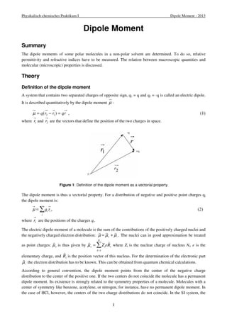
A system that contains two separated charges of opposite sign, q1 = q and q2 = -q is called an electric dipole.
It is described quantitatively by the dipole moment μ :
= q(r − r ) = qr μ 2 1 , (1)
where r1 and r2 are the vectors that define the position of the two charges in space.
Figure 1: Definition of the dipole moment as a vectorial property
The dipole moment is thus a vectorial property. For a distribution of negative and positive point charges qi
the dipole moment is:
μ = qi ri
i
where i r are the positions of the charges qi.
The electric dipole moment of a molecule is the sum of the contributions of the positively charged nuclei and
the negatively charged electron distribution:
r
μ =
r
μ + +
r
μ −. The nuclei can in good approximation be treated
as point charges:
r
μ + is thus given by
r
R i
NΣ
r
μ + = Zie
I =1
where Zi is the nuclear charge of nucleus Ni, e is the
elementary charge, and
r
R i is the position vector of this nucleus. For the determination of the electronic part
r
μ − the electron distribution has to be known. This can be obtained from quantum chemical calculations.
According to general convention, the dipole moment points from the center of the negative charge
distribution to the center of the positive one. If the two centers do not coincide the molecule has a permanent
dipole moment. Its existence is strongly related to the symmetry properties of a molecule. Molecules with a
center of symmetry like benzene, acetylene, or nitrogen, for instance, have no permanent dipole moment. In
the case of HCl, however, the centers of the two charge distributions do not coincide. In the SI system, the

2. Physikalisch-chemisches Praktikum I Dipole Moment - 2013
unit of the electrical dipole moment is C×m. Since these units result in very small numbers, the unit Debye
(1D = 3.33564×10-30 Cm) was introduced in honor of the discoverer of the dipole moment, Peter Debye
(1911-1912 Professor of theoretical physics, University of Zurich).
Two elementary charges (e = 1.602×10-19 C) of opposite sign placed at a distance of 1.28 * 10 -10 m, i.e. the
bond length of the HCl molecule, give rise to a dipole moment of 6.14 D. This represents a purely
electrostatic model for the ionic HCl structure. In practice, however, only a dipole moment of 1.08 D is
found. The molecule is thus only partially ionic. The ionic character X describes partially ionic chemical
bonds:
2
X =
μ(measured)
μ(calculated)
×100%, (3)
for example X of HCl is 17.6%. Experimental dipole moments provide information about the electron
distribution in a molecule.
In this experiment dipole moments of some polar molecules in non-polar solvents are measured and
discussed. This is practically done by measuring relative permittivity and refractive indices of solutions and
pure solvents. The relation between these two macroscopic properties and the molecular dipole moment is
discussed in the following.
Relative permittivity, Polarization, and Polarizability
Between two charged plates of a capacitor there is an electrical field. If the distance between the two plates is
much smaller than the surface of the plates, the field can be considered homogeneous except in the border
regions (Figure 2). The electrical field strength E0 is given by
0 s /e
0 0
= =
S
e
0
q
E , (4)
where s 0 = q/S denotes the surface charge density of one condenser plate (S = surface area, q = charge on
one plate) and e0 is vacuum permittivity (e0 = 8.85419 10-12 J-1C2m-1). The voltage U0 between the two plates
is proportional to the charge q:
Figure 2: Electrical field in a capacitor
q = C0 ×U0. (5)
The proportionality factor C0 is called capacity. The following equation relates C0 and the field strength E0:
C0 = q/U0 = q/(E0 × d) . (6)

3. Physikalisch-chemisches Praktikum I Dipole Moment - 2013
C0 is thus proportional to 1/E0 provided charge q and plate separation d remain constant.
Experimental observation
As a capacitor is filled with matter, the voltage U between the two plates is reduced from the voltage in
vacuum, U0:
U = U0/e , E = E0/e, and thus C = e C0 (7)
with e > 1. e is the so-called static relative permittivity of the filled in material (dielectric) and is a material
constant.
In order to explain this behavior we introduce the polarization
3
r
P of a dielectric in a field
r
E 0. It is defined as
follows
r
P =e0(
r
E 0 −
r
E ) =e0(e −1)
r
E (8)
and is a vectorial quantity.
r
E 0,
r
E , and
r
P are parallel. Inserting (4) into (8) one gets the scalar relation
E = (s 0 − P)
e0
def s
=
e0
. (9)
The electric field E with a dielectric can thus be described as the field in vacuum. Its strength does not
correspond to the surface charge density s 0 any more but to a reduced density s (s = (s0 – P)). Polarization
can thus be regarded as a surface charge density that is induced by field
r
E 0 on the interface between
dielectric and capacitor plates. This induced charge density s partially compensatess 0 because these charges
have opposite sign. The so-called free surface charges are caused by three processes, which arise at the
molecular level under the influence of an electric field. The observed polarization P can thus be regarded as
being the sum of three contributions:
P = PD + PE + Pμ . (10)
Electronic polarization PE :
i
μPis found in all atoms and molecules. It is caused by the fact that the centers of positive charges (nuclei)
E and negative charges (electrons) are pulled in different directions in an external field.
Distortion polarization P:
D This contribution is only found in polar molecules and is caused by changes in bond lengths and angles.
Pand Pare combined to the so-called displacement polarization which is caused by distortion of a
E D molecule in an external electric field E. Due to such a distortion a molecular dipole moment is induced.
As long as the external field is not too strong, we can assume
μi
=aE . (11)
i
The proportionality μfactor a is called the polarizability of a molecule. It indicates how easy a molecule can
be distorted. In liquid solutions the induced dipole moment is always oriented in direction of the external
field.
Orientation polarization Pμ :

4. Physikalisch-chemisches Praktikum I Dipole Moment - 2013
Pμ is only found in polar molecules with a permanent dipole moment
4
r
μ 0 . It is caused by a partial alignment
of the molecular dipole moment into the direction of the external field. In contrast to PD and PE , Pμ varies
strongly with temperature since the thermal motion is opposite to the alignment.
In an external electric field, polar molecules have thus a total dipole moment
r
μ according to
r
μ =
r
μ 0 +
r
μ i . (12)
Our model of a dielectric between two charged capacitor plates can now be sketched as shown in
Figure 3. We hereby denote a molecular dipole moment by . It explains the free surface charges q’ at
the dielectric boundary surface S. P can then be written as:
q d
V
×
q d
S d
P q S
×
=
×
= =
' '
-+-
' / . (13)
Figure 3: Simple model of a dielectric
μ r
P can be regarded as the electrical dipole moment (q’·d) per unit volume V of the dielectric, which due to the
molecular dipole moments corresponds to the vector sum:
j Σ
=
=
l N
j V
j
P
1
1
μ r
r
, (14)
where Nl denotes the number of molecular dipole moments in volume V and each individual dipole moment
j μ r
comes from equation (2). Equation (14) provides an interpretation of the macroscopic property
r
P in
terms of molecular (microscopic) properties.
The Debye equation
In 1912 Debye developed a theory for the relation between the polarizability a, the permanent dipole
moment μ0 and the relative permittivity e of a substance. He found the following formula:
e −1
e + 2
M
r
=
NL
3e0
a +
μ2
0
3kT





 , (15)
where M denotes the molar mass, r the density, NL Avogadro’s number, and μ0 the permanent dipole
moment. The first term in parentheses corresponds to the distortion polarization and the second term to the
orientation polarization. One notes that the latter contribution becomes smaller with rising temperature, a
consequence of thermal motion. This so-called Debye equation (15) neglects polar interactions of dipoles
with their surroundings. It is therefore valid only for dilute solutions of polar substances in non-polar
solvents and for polar gases at pressures smaller than 1 atm.

5. Physikalisch-chemisches Praktikum I Dipole Moment - 2013
The Debye equation is the basic equation for the determination of molecular dipole moments in non-polar
solvents. It order to apply it, however, polarizabilites a of solvent and solute molecules have to be known.
To determine these quantities, the refractive indices of solvent and solute molecules have to be measured.
Dispersion of the Polarizability and the Relation between e and n
Dispersion of the polarization
Dispersion generally means the frequency dependence of a physical quantity. The displacement of charge in
a molecule due to an external field causes an induced dipole moment μi
5
=aEi . This effect, as well as the
orientation of the permanent dipole moments, is achieved in a finite time. The same is valid for the reverse
case, namely if the polarizing field is switched off and the molecules return into their non-polarized
disordered initial state. The so-called relaxation time t indicates how much time is needed until the
polarization effects are reduced to 1/e after the external field has been switched off. Typical relaxation times
of different polarizations are listed in Table 1. Pμ obviously depends on the viscosity of the medium.
Table 1: Relaxation times at different frequencies and in different media
polarization size of
molecule
medium t [sec] frequency
PE 10-15 UV
D P
10-12-10-14 IR
Pμ
gas 10-12 far IR
Pμ small solution, low
viscosity
10-10-10-11 microwaves
Pμ large solution, high
viscosity
10-6
Pμ glasses up to hours
radio frequencies
The Debye theory is only valid if the polarizing electrical field changes slowly enough such that polarization
and orientation of the molecules are always in equilibrium with the field. This condition is fulfilled with
certainty in a static field or in solutions of low viscosity. Also, an alternating radiation field with a frequency
of 106 Hz fulfils this condition since the relaxation time t is much smaller than 1 μs as seen in Table 1. From
frequencies larger than 1010 Hz also the atomic polarization disappears (see Figure 3) and at frequencies
higher than ca. 1014 Hz, only electronic polarization is left. P and thus also e depend on the frequency and the
contribution of electronic polarization can be determined by measuring e at light frequencies of 4 to 8×1014
Hz. Figure 4 depicts schematically the discussed dispersion of the polarization.
Figure 4: The dispersion of polarization

6. Physikalisch-chemisches Praktikum I Dipole Moment - 2013
The relation between n and e
From Maxwell’s theory of electromagnetic waves follows an expression for the phase velocity n of a light
wave in a medium with relative permittivity e and a magnetic susceptibility μm:
6
n =
c
e ×μm
(16)
where c is the speed of light in vacuum. The refractive index n of this medium is defined by:
n =
sina
sinb
=
c
n
(17)
n is thus always ≥ 1.
§
α = angle of incidence
β = angle of refractive
n = speed of light in medium
Figure 5: Refraction of
light
For many organic substances μm deviates only very slightly from 1, we can therefore write in good
approximation:
n =
c
e
(18)
or
n2 =e (19)
The relative permittivity corresponds thus to the square of the refractive index n. Its magnitude and
frequency dependence are a measure for the achievable electron polarization and its relaxation time.
The Guggenheim approximation
For a completely independent determination of the polarizability a in (15) the contribution of distortion
polarization should be determined. This is however difficult to do. The Guggenheim approximation 2,3 allows
approximate calculation of dipole moments of polar molecules in non-polar solvents. It is based on the
Debye equation and makes the determination of
r
μ 0 possible solely by measuring e and n2. Hereby, it is
assumed that the distortion polarization of a molecule is proportional to its molar volume. The Guggenheim
approximation reads
2 =
μ0
27kT
NL
e0
1
r1
(e1
+ 2)(nD1 + 2)
× M2 × (be − bn ) (20)
with
be =
de
dw2
and
( 2 )
dw
2
d n
b D
n = (21)

7. Physikalisch-chemisches Praktikum I Dipole Moment - 2013
The physical properties of the pure solvent are labeled with 1 and those of the dissolved substance with 2. nD
is the refractive index at the frequency of the sodium D-line and w2 = m2 / (m1 + m2) is the weight fraction of
the dissolved substance. The obtained experimental data is analyzed according to this Guggenheim equation.
To do so, one needs the density (r1), the relative permittivity (e1) and the refractive index (nD1) of the pure
solvent. The slopes e b and n b are obtained by plotting ε and nD
n = (22)
7
2
against the weight fraction w2.
Experimental Part
Dipole- and refractometer needed used during the experiment have to be kept very accurately at the same
constant temperature.
The Dipole Meter
In this part of the experiment, we want to determine the relative permittivity e at low frequencies, i.e. in the
region of radio waves (~106 Hz). In this spectral region, all contributions to the polarizability are effective
(see Fig 4). To do so, we use a dipole meter, which consists of a resonant circuit that oscillates at its
eigenfrequency:
1
LC
1
p
2
The eigenfrequency is measured with a frequency counter. Filling the capacitor with a liquid changes C
according to (7):
C = eC0
We can thus rewrite Eqn. 22 to
n =
1
2p
1
LC0e
=
1
4p 2LC0e
= k
e
(23)
by merging all the constant terms into a constant factor k. This finally reveals the relation between the
frequency readout and the relative permittivity:
e =
k
n 2 (24)
After calibration with a liquid of known relative permittivity e,
the proportionality constant k can be
determined.
Experiment
The eigenfrequency of the pure solvent with known relative permittivity e (heptane, eheptane = 1.924 –
0.00140[T – 200C] is measured first (at least three measurements). With the obtained frequency n, the
constant k of the experimental setup is calculated. Then the eigenfrequency of each solution is measured at
three different concentrations (only once) and the corresponding permittivities are calculated as described
above. Then, e is plotted against the weight fraction w2 (not the percentage) and the slope be is obtained:
be =
de(n radio )
dw2
=
d


k
n 2




dw2
(25)

8. Physikalisch-chemisches Praktikum I Dipole Moment - 2013
The Refractometer
According to Maxwell’s theory, the relative permittivity e(n) in the visible region of the electro-magnetic
spectrum can be easily determined using optical methods by measuring the refractive index at a given
frequency. As shown in Fig. 4, in this part of the spectrum, the electronic polarization dominates and no
contributions from orientation polarization or distortion polarization exist.
The refractive index is measured with a refractometer as proposed by Abbé. The technique is based on the
phenomenon of total reflection. A light beam with an incidence angle a in medium 1 hits a phase interface
to an optically less dense medium 2. The angle of refraction b in medium 2 is thus larger than a.
Using a relative angle of refraction
8
n =
n1
n2
=
sinb
sina
>1
For normal refraction the relation
0 £ n × sina = sinb £1
always holds. An incident angle a0 < 900 must thus exist with
sin 1/ n a0 =
If light hits a phase interface with an angle a0, the refracted light streaks the interface (b = 900). In case of
angles a > a0 the light beam is reflected at the interface. a0 is called the critical angle for total reflection.
The Abbé refractometer (Figure 5) contains two prisms made of vulnerable flint glass of high optical density
(large n1), a prism for illumination and one for detection, a traversable telescope adjusted to infinity, and a
lamp. The sample is in a layer with a thickness of 0.1 mm between the two prisms.
Figure 6: Sketch of an Abbé refractometer
The incident light through the lighting prism is scattered on the matte finished bottom side such that the
probe is irradiated largely isotropically. Some light hits the detection prism under the critical angle of total
reflection. For larger observation angles, the detection prism appears dark. The angle distribution of the
leaving light is observed using a traversable telescope that is adjusted to infinity. In contrast to a microscope,
not all the light that originates from one point of the examined object is mapped on one point of the eye’s
retina but all the light that enters the telescope with the same angle. Since white light is applied and since the

9. Physikalisch-chemisches Praktikum I Dipole Moment - 2013
refractive index varies with frequency (dispersion) no clear bright-dark edge appears in the visual field of the
telescope, but a blurred coloured fringe. Using a compensator this fringe can be turned into a distinct bright-dark
9
edge.
This compensator consists of two parts, each one consisting of three Amici prisms that can be twisted against
each other. This construction reveals a system of variable dispersion that can be used to calibrate the
dispersion of lighting and detection prisms. To do so, the cross wire is adjusted on the bright-dark edge and
the refractive index can directly be read on the shown scale.
Experiment
First the refractive index of the pure solvent is measured as a reference. Then, the refractive index of each
solution is measured for three different concentrations (the same solutions as for the dipole meter
measurement are used). With the obtained refractive indices n, the relative permittivity e = n2 is the visible is
calculated. Then e is plotted against the weight fraction w2 (not the percentage) and the slope bn is
determined:
2
( ) ( )
2
e n
2
d n
dw
dw
d
b vis
n = =
(26)
With bn and be all variables are known in order to calculate μ0 according to the Guggenheim approximation.
Carrying out the experiment
At the beginning, turn on the dipole meter and thermostat. The apparatus has to reach a thermal stationary
state before measurements can be made. This takes about 15 min. The temperature of the thermostat may not
change by more than 0.1° C during the experiment. Otherwise, the measurements of refractive index and
capacity are not sufficiently precise.
Meanwhile, prepare three solutions of the substance received from the assistant in heptane according to the
following procedure: In a 50 mL graduated flask weigh about 49 mL (accurately!) of heptane. Then, using a
syringe, add as much sample as you need to obtain a weight fraction of about 3%. 15 mL of this solution is
put into a second flask (weighed exactly!). The remaining 35 mL are stored well closed and used later on for
determining e and n. Dilute the 15 mL with solvent to 50 mL and weigh again in order to exactly determine
the weight fraction. It should be approximately 1%. Apply the same procedure to prepare a solution with a
weight fraction of about 0.3%.
It is very important that the solutions are prepared exactly according to this instruction!
Use a 20 mL syringe and plastic tube to fill the cell with solution or solvent. Do it carefully and make sure,
that no liquid is spilled at the top of the cell. Any air captured in the cell would disturb the measurement.
After filling in solvent or solution, always wait about 5 min until the solvent is in thermal equilibrium with
the apparatus. Then read off the eigenfrequency from the frequency counter.
As a first measurement, determine the relative permittivity of the pure solvent. For this purpose fill the
measuring cell with heptane. Read off the frequency at least three times and take an average result. From the
measurement, determine the constant k in Eqn 24. In all subsequent measurements of solutions, it has to be
ensured that the cell is clean and dry before a solution is filled in so that the concentrations are not changed.
The cell has to be blown out with the dryer first hot, then cold, until no solvent can be smelled. After
one measurement, the cell is cleaned with solvent and the solvent is measured again. Finally, a plot is
generated according to Eqn. 25.
In parallel, determine evis by measuring the refractive indices of solvent and solutions. Using a pipette solvent
or solution is put on the detection prism. Then, put on the lighting prism using the bayonet nut connector.
Clean the prisms using Linsoft tissues and acetone or ethanol. Take care not to scratch the prisms!

10. Physikalisch-chemisches Praktikum I Dipole Moment - 2013
Make a plot according to Eqn. 26. The density r1 of the solvent is given below and the molar weight of the
dissolved substance M2 is known. All variables in order to calculate μ0 according to the Guggenheim
equation are now known.
10
Practical Advice
Preparing the solutions
• The indicated concentrations do not have to be exactly those specified, but they have to be known
exactly.
• Check carefully that pipettes, flasks, etc are clean.
• Use different pipettes for different substances.
• Always close the flasks to avoid change of concentration due to evaporation.
• Keep the solutions after the measurements in case you have to repeat some of them.
General remarks
• All constants are in the SI system:
e = 1.602177 10-19 C
e0 = 8.85419 10-12 J-1C2m-1
• Begin with low concentrations and move consequently to higher ones.
• When the concentration is changed, the cell has to be rinsed twice with pure solvent, be dried with the
dryer until you cannot smell any solvent.
• Check carefully the temperature during the whole experiment.
Wait ten min. after a solution has been filled in such that thermal equilibrium is reached.
• Repeat every measurement three times and average the results.
• e1 = eheptane = 1.924 – 0.00140[T – 200C]
r1 = rheptane = 0.681 g/cm3
M1=Mheptane= 100g/mol
d = bond length C-Cl = 1.77Å
J2 = 55°53’
J3 = 72°0’
Tasks
1. Determine the dipole moments of chloro-cyclohexane, dichloromethane, trichloro-methane
(chloroform) and monochloro-benzene. Compare your values to reference values from the literature.
2. The calculated dipole moment of chloro-cyclohexane (μ1) is used to determine the ionic character of
the C-Cl bond:

11. Physikalisch-chemisches Praktikum I Dipole Moment - 2013
11
J =
μ1
d × e
(d = bond length C-Cl, e = elementary charge)
3. The deviation from the vector sum due to alternating induction should be determined for the dipole
moments of dichloro-methane (μ2) and trichloro-methane (μ3).
Dμ=μ2 - 2μ1 cos(J2)
Dμ=μ3 - 2μ1 cos(J3)
J is the angle between the individual bond dipoles and the vector sum
4. Determine the reduction of the dipole moment (μM) due to resonance in monochloro-benzene:
Dμ = μ1
−μM
Literature:
1. G. Wedler, Lehrbuch der Physikalischen Chemie, 2. Auflage, VCH Verlagsgesellschaft,
Weinheim, 1985
2. P.W. Atkins, Physical Chemistry, 5. Edition, Oxford University Press, 1994
3. C.F.J. Böttcher, Theory of Electric Polarization, 2. Edition, Elsevier, New York, 1973 and
1978.
4. H.B. Thompson, The Determination of Dipole Moments in Solution, J. Chem. Educ. 1966,
Vol.43, pp. 66 - 73